Agent-based Multi-layer Network Simulations for Financial Systemic Risk Measurement: a Proposal for Future Developments
- Università degli Studi di Macerata, Italy
Abstract
The paper addresses the topic of measuring the systemic risk and of identifying Systemically Important Financial Institutions (SIFIs) with an agent-based multi-layer network simulation. The paper starts from the shortcomings of the models currently proposed in the literature and suggests directions for future researches and guidelines to realize a methodology able to accurately model the direct network contagion channel (interconnectedness of balance sheet of financial institutions, including direct losses and liquidity hoarding), also integrating the indirect contagion channel (fire sales and bank runs), in order to reach the full representation of the financial systemic risk.
1) Introduction
The development of a methodology able to accurately quantify systemic risk and identify the Systemically Important Financial Institutions (SIFIs)1 is of paramount importance for two reasons: (i) the distress of a SIFI can trigger a financial crisis and, consequently, a large and prolonged real economic crisis; (ii) current regulation requires additional capital requirements for SIFIs, modifying their behaviour (and their performances) with consequences on the real economy as well.
Regulators and academic authors are proposing various methods to detect SIFIs, but these methodologies feature many shortcomings and are not consistent among themselves in ranking the systemic importance of the analysed FIs, as shown by many studies (such as Benoit et al., 2017; Brogi et al., 2021; Grundke, 2018; Löffler and Raupach, 2013; Nucera et al., 2016). As explained by Hansen (2014), there should be a concern for robustness, because model misspecification can result in flawed policy advice. Therefore, a final shared methodology is still a very relevant open issue.
This paper suggests to perform an agent-based multi-layer network simulation, trying to fill the gaps found in the literature. Indeed, starting from the shortcoming of the current simulations, the paper advises some guidelines for future improvements of agent-based multi-layer network simulation, to reach the ground-breaking target of a full representation of the systemic risk, in order to:
assess the potential systemic losses due to a shock or due to a bank default;
detect and rank SIFIs depending on their systemic importance;
give an early warning signal of financial fragility to supervisors;
assess which macroprudential and microprudential interventions by financial regulators are most effective in avoiding the spreading of financial distress among FIs, and study if a regulatory framework reduces or increases the systemic risk.
The proposed methodology is based on a simulation procedure in which the regulator can insert a shock and observe the consequences for the (almost) whole financial system. Indeed, when possible (that is for specific topics), in my opinion, economists should follow the methodology often used in natural (or “hard”) sciences which have been applying simulations for decades (see, for instance, the simulation methodologies used for weather forecasting). Neveu (2016) also suggests to “use methods similar to the stress test methodology (…) using a variety of narrow and broad shocks” to stress the calibrated model. Moreover, adopting the complexity approach of agent-based models, the methodology is suitable to represent non-linear outcomes and evolution of agents, generated by their mutual interaction within a changing environment.
The paper proposes a broad view and a direction for future research, including suggestions about how to integrate different models and approaches to overcome the limitations that each of them have. The development of a methodology able to follow the guidelines proposed in this paper, will have a relevant impact both on academic studies on systemic risk and on the methods actually applied to detect SIFIs by financial regulators worldwide.
The paper is structured as follows. Section 2 presents a literature review focused on network based approaches. Section 3 explains the methodology to model the systemic risk, and Section 4 concludes.
2) State of the art and proposal starting points
Even if some early papers tackled the issue of systemic risk (for an early survey see de Bandt and Hartmann, 2000), recently the literature on this topic had shown an exponential growth. Indeed, the various features of the systemic risk topic (sources, mechanisms, measurement approaches…) are analysed in an enormous (and continuously growing) number of papers. Some papers, such as Silva et al. (2017) and Benoit et al. (2017), try to review this literature.
Sources and mechanisms are by now well established. The systemic risk is provoked by the direct and indirect contagion channels explained by Gai and Kapadia (2010). In each of these two channels, two mechanisms can be distinguished; therefore, the systemic risk channels can be summarized as follows:
the direct contagion risk due to the network of exposures within the financial system. This can create both a liquidity risk due to liquidity hoarding, and a solvency risk due to losses related to defaulted or troubled FIs;
the indirect contagion risk caused by bank runs phenomena and fire sales of common assets. Bank runs are related to the liquidity risk, while fire sales of common assets cause losses and therefore are mainly related to solvency risk (but also to liquidity risk through the “haircut”2 mechanism).
However, there is still a large debate about methodologies that have to be used to measure systemic risk. Given the presence of the cited literature reviews, I will only perform a detailed review of the systemic risk literature strands on network approaches. This methodology is completely different from the most cited measures that try to quantity with few factors the effects of all the systemic risk channels. Two famous examples of these measures are the Acharya et al. (2012) and Brownlees and Engle (2017), and the Adrian and Brunnermeier (2016). These measures are often based only on market prices used as a proxy able to include all channels of systemic risk. However, these methods are often criticized, mainly because they:
have weak theoretical foundation, as stated by Nucera et al. (2016);
focus only on a few aspects and channels of the systemic risk (also compared to the Basel Committee approach), and “neglect to take many aspects of complexity into account” (Neveu, 2016);
use very strong assumptions and/or lack of robustness to changes in the assumptions (see the relevance of the “model risk of risk models” explained by Danielsson et al., 2016);
are often based on market data (stock price, CDS spread…) unavailable for many FIs;
are unable to be early warning indicators, as highlighted by Di Iasio et al. (2015): “several critics argued that these asset prices-based indicators might perform well as thermometers (coincident measures), but not as well as barometers (forward looking indicators)”.
For a discussion on these shortcomings, see Brogi et al. (2021).
2.1) Network based approaches and their weaknesses
The network theory is probably the best tool for analysing the contagion risk. Indeed, the financial system is well suited for a representation with basic network theory, in which nodes represent institutions and links represent relations (credit and liabilities, derivatives…), as explained, for instance, in Shleifer and Vishny (2010). In particular, the direct contagion risk can be accurately analysed using a directed and weighted multi-layer network, while the fire sale mechanism can be well approximated starting from a bipartite and weighted multi-layer network of common exposures. In other words, three of the four mechanisms explained above are due to the network of mutual exposures; only bank runs could develop without network relations. Consequently, researchers and policy makers at central banks are becoming more and more interested in network analysis, supporting network-related research.3 The importance of network theory for systemic risk measures is highlighted by Neveu (2016), who performs a survey of systemic risk literature based on the network approach (previous surveys of the literature on contagion in financial networks are Cabrales et al., 2015; Glasserman and Young, 2015; Hüser, 2015). Most network theory papers on the financial system focus specifically on the interbank credit market (but there are papers also on firm-bank credit relationship, such as Bargigli et al., 2014b; Bargigli et al., 2018): the interconnectedness of FIs is a source of credit risk on interbank markets, that can cause the problem of contagious defaults. While earlier contributions (Allen and Gale, 2000) stressed the benefits of increasing diversification, suggesting that the more connections there are the better for financial stability, later works have challenged this view, showing that diversification is not always beneficial for stability, and underlining instead the systemic risk provided by default cascades and other contagion effects. For instance, Battiston et al. (2012a) show that, if a financial accelerator mechanism is present, then a potential trade-off between individual risk and systemic risk may exist due to the increasing connectivity of the network.4 Similar results are provided by Gai and Kapadia (2010), who show that financial systems exhibit a robust-yet-fragile tendency: while the probability of contagion may be low, once a default cascade is started its spread can be quite large. In other words, credit network plays two different roles at the same time: on the one hand, it is useful for its risk-sharing effect, while on the other hand, it may be dangerous for its contagion effect. The problems arising from financial market interconnectedness have also been highlighted by studies such as Cocco et al. (2009), Gai et al. (2011) and Di Iasio et al. (2015).
In the last few years, many papers have extended the analysis from a simple single layer network to multi-layer networks (see Bargigli et al., 2014a; Molina-Borboa et al., 2015; Poledna et al., 2015; Montagna and Kok, 2016; Aldasoro and Alves, 2018; Huser and Kok, 2020; Huser and Kok, 2020; Covi et al., 2021). Multi-layer networks feature a layer for each kind of asset, disaggregating them into groups with different seniority or maturity. Hüser et al. (2018) find that “the network layers have very different link structures and there is strong heterogeneity in the significance of banks in the different layers”, therefore this disaggregation is of paramount importance. Molina-Borboa et al. (2015) show that focusing on a single layer severely underestimates total systemic risk computed with the DebtRank measure developed in Battiston et al. (2012b). Bookstaber and Kenett (2016) find a similar result. Therefore, one detailed large model is preferable to a number of small models, each describing a specific asset, kind of institution or risk of the financial activity. For instance, the U.S. Securities and Exchange Commission (SEC) produced a staff report to review how markets behaved during the Covid-19 pandemic crisis (Kothari, 2020). The report finds interconnections in many ways among the various U.S. credit markets, which raises the concerns for the spillover of risks and shocks from one market to the others.
In general terms, the dynamics of any contagion process depends crucially on network topology. In this context, heterogeneity becomes of paramount importance: some nodes may be too big or too connected to fail. Empirical analyses, such as De Masi et al. (2015) or Cont et al. (2013), find unequivocal evidence of heterogeneity in credit networks. Therefore, a specific network heterogeneity needs to be addressed besides node heterogeneity to get a deeper understanding of which institutions are systemically important. Then, the modelling framework should be grounded in the empirical evidence, using real data as stressed by Ramadiah et al. (2020), who find that observed credit network displays higher levels of systemic risk compared with most networks built with reconstruction methods starting from partial network information.
However, the analysis of the contagion dynamic in presence of a network calibrated on real data (with heterogeneous nodes, especially in the case of a multi-layer network) is a hard task because of the presence of numerous nonlinearities. Therefore, a feasible way to address the complexity of the contagion in a network of heterogeneous and interacting agents is to simulate its dynamics. Many network studies (see the already cited literature reviews, such as Neveu, 2016) simulate what happens to the financial system, for instance, if one bank defaults due to an exogenous shock: this event determines bad debts to other banks in the interbank markets, that can go bankrupt with a new round of losses and so on, possibly causing a bank default cascade. The methodology proposed in this paper starts from some of these papers using simulations: Gai et al. (2011), Battiston et al. (2016); Battiston et al. (2012b), Manna and Schiavone (2012), Poledna et al. (2015), Montagna and Kok (2016), Hüser et al. (2018), and Covi et al. (2021).
One of the starting points is the “DebtRank” measure of Battiston et al. (2016); Battiston et al. (2012b). This measure, applied in many papers such as Di Iasio et al. (2015), is the first measure able to address the problem of distressed, but non-defaulting, institutions. Glasserman and Young (2015) find that this channel of contagion is considerably more important than effects due to defaults. For instance, as explained in Di Iasio et al. (2015), a bank that suffers high losses (but does not default) shortens its distance-to-default and reduces the market value of its stocks and bonds; then, other banks that own these financial instruments in the “trading book” will be required to cut the mark-to-market value with further losses. Therefore, DebtRank expresses the fraction of the total economic value of the network - excluding bank i - posed at risk by some exogenous shock that hits bank i. This measure has two advantages compared to other algorithms, as highlighted by Battiston et al. (2012b): it is a possible early warning indicator because it delivers a clear response well before the peak of the crisis, and it has the precise meaning of economic loss, measured in dollars, caused by a shock.
However, the DebtRank measure used in the cited papers does not include three of the four contagion mechanisms explained, that is it addresses only the “direct losses”. Consequently, it does not consider the liquidity risk.
Moreover, Battiston et al. (2012b) determine the impact of a negative shock on a bank considering the equity relations between banks as a proxy of the overall relations. In practice, if bank A loses α% of its equity value, than bank B, that owns some stocks of A, suffers a loss on its capital equal to a multiple of α% of the value of the A equity owned, representative of its exposure towards bank A in equity, credit and other instruments. This is an over-simplifying assumption due to the lack of data, that probably overestimates the effect of the shock. A real assessment of the whole asset side of a bank should be carried out, and for each kind of exposure a different loss has to be associated with a loss on the bank equity. Indeed, for instance, the value of the bond of a bank could be reduced only by a small fraction, even if the stock market value of that bank decreases by a large percentage. Moreover, the relationship is highly nonlinear and, even in case of default, the value of a bond could not go to zero thanks to the recovery rate (RR), that instead is assumed equal to zero in Di Iasio et al. (2015). Poledna et al. (2015) uses the DebtRank measure applying a fixed loss given default (LGD), but it is again an unreliable assumption given that the LGD increases in presence of stronger crises. However, Poledna et al. (2015) extend the DebtRank measure to a multi-layer simulation. Indeed, they build a layer of exposures for derivatives,5 alayer of securities issued by banks and hold by other banks, a layer for the settlement risk on foreign exchange exposures, and a layer for interbank deposits and loans.
Another weakness of the DebtRank measure, that can underestimates the effect of the shock, is the assumption that contagion cannot repeat an “edge” between two “nodes” in order to avoid the risk of possible infinite reverberations due to loops among nodes.
Battiston et al. (2012b; 2016) miss the importance of banks’ balance sheets and the related regulatory constraints that banks have to comply with, together with the strategies that banks can perform to avoid the default. Actually, FIs have to reply to the shock, that reduces their equity or their liquidity, taking corrective action on their balance sheets, that is usually reducing their assets. Gai et al. (2011), and Manna and Schiavone (2012) are the first examples of the few papers that address the issue of considering the behaviour of banks in complying with regulatory constraint. In other words, they are the first agent-based models, that is models in which agents actively behave.
Moreover, Manna and Schiavone (2012) address the fact that banks’ balance sheet is composed of different assets and liabilities, articulating them in many important items. They build a simulation in three stage able to show the problems of defaulted, illiquid and undercapitalized banks.
Besides some over-optimistic assumptions, this approach does not consider endogenous solutions for the price of the securities held by banks, so as to mark-to-market their assets, as (approximately) done in the DebtRank procedure. This is very important both for assets that banks are forced to sell, but also for assets that remain in the balance sheet and could carry losses, because they are in the “trading book” evaluated mark-to-market or they are in the “banking book” and the book value of the most problematic exposures is reduced with an “impairment test”.
Hüser et al. (2018) perform a similar simulation approach, even if they restrict their simulation to this first stage of Manna and Schiavone (2012) only, without considering the strategies that FIs can implement when they are in trouble. In particular, exploiting some European Central Bank (ECB) datasets, they use a real network to analyse the bail-in of each systemic Euro area banking group, and find that it does not imply direct contagion to creditor banks. This is in line with the findings of all the papers using the network simulation approach: they generally highlight that contagion due to the direct interbank network exposure is likely to be rare. Moreover, it happens only when very strong assumptions are at the base of the simulations, that is if: (i) the initial shock is the collapse of the largest bank in the country, (ii) there is no transfer of resources within banking groups, (iii) there is no government support, and (iv) the loss-given-default is very high, as explained also in Manna and Schiavone (2012).
Another important limitation of the analysed papers is that they do not include an assessment of the fire sale mechanism. Montagna and Kok (2016) add this assessment endogenously determining the price of the securities held by the FIs as a function of the amount sold by the institution and of the depth of the market for that security. However, they lack the impact of distressed but non-defaulting institutions and utilize only three layers (short and long term debts, plus common exposures to assess fire sales).
In conclusion, the most relevant and common methodology limitations (avoiding to mention other minor problems, often specific to each paper) which emerge in the recently proposed simulation approaches are:
lack of a “real” balance sheet of the analysed FIs (a “real” assessment of asset and liability sides, including a subdivision between trading and banking book);
lack of an endogenous peculiar estimated loss (and of an endogenous RR when needed) for different kinds of instruments, including both assets issued by the analysed FIs and other assets fire sold;
lack of the impact of distressed, but non-defaulting, institutions;
lack of the full set of regulatory constraints;
lack of a reliable reaction behaviour of all agents involved in the simulation, including distressed FIs, non-distressed FIs (that can perform liquidity hoarding), and non-financial agents (that can perform bank runs).
Many papers solve some of the previous shortcomings, but none of them face all the limitations at the same time. Therefore, there is the need to implement a methodology able to consider all the raised issues in a reliable way, in order to reach a full representation of the financial systemic risk channels.
Moreover, the reviewed simulation approaches are (sometimes)6 empirically applied to a relatively small set of FIs. Therefore, there is the need to implement the methodology:
considering the relevant exposures of all banks (not only the Global Systemically Important Banks - G-SIBs; for instance, given the core-periphery structure of the banking system, the default of a medium bank that is the “hub” of a cluster of regional banks can be more relevant than the default of a large bank) and of all the relevant FIs (for instance, large insurance companies, large mutual / money market / pension / sovereign wealth funds). Neveu (2016) points out that risk measures are useless when considering the robustness of a system that includes very large unmonitored sectors;
integrating the approach globally. Indeed, Montagna and Kok (2016) explain that: “If the ultimate goal is to reduce systemic risk, it is necessary to have a global view of the financial system in order to identify and monitor possible sources and channels of contagion.”
3) The proposed methodology
I propose an agent-based multi-layer network simulation methodology in order to have a strong and theoretically sound methodology able to model all systemic risk channels. The methodology should apply some of the best practices developed in the cited literature strand on network based approaches.
The proposal is addressed to central banks and global financial regulators for two reasons: the need of confidential data and the need of a strong team, as explained in Subsections 3.1 and 3.2.
3.1) The need of confidential data
The proposed methodology relies on balance sheet data that should be provided by the financial regulator. Covi et al. (2021) explain that “because of the confidential nature of this data, the access is generally restricted to banking supervisors and central banks”.
Central banks do not rely on academic methods based on market data because of the problems already explained in Section 2, while they support studies on network approaches and based on accounting data. However, accounting data feature some problems too. First, accounting rules are different in different countries, as pointed out by Iwanicz-Drozdowska (2014). Second, accounting data are disclosed with a lag, and it is a problem because they could be unable to work as early warning indicators. Third, the data should be granular enough and should be collected not only for G-SIBs, but also for less relevant banks and non-banking SIFIs, and at global level, as explained in Subsection 2.1. Therefore, the data issue is crucial both to make network simulations really feasible and in a timely manner. I can summarize the three reported issues as the need of standardised, timely and “big” (granular and for all relevant FIs at global level) data.
However, financial regulators are already going in the right direction with many initiatives on data reporting and collection. For instance, in the USA, the Dodd-Frank Act established the “Office of Financial Research” (OFR) to collect data on the financial network in order to detect the SIFIs, plan policy interventions, and disclose data to the financial markets.7 In the EU, the ECB, starting from the 2014 “Comprehensive Assessment”, collects asset side information, trying to uniform balance sheet schemes and reporting data from different countries. Moreover, subsequently to the 2008 G-20 at Washington D.C., the EU approved the EMIR (Regulation 648/2012), the MiFIR (Regulation 600/2014) and the MiFID 2 to force a better disclosure and a centralized negotiation in regulated markets with a clearing house even for some over-the-counter derivatives. Nevertheless, to obtain the required global view, an acceleration in the unification of the accounting standards is being carried out thanks to the G-20 Data Gaps Initiative (DGI) led by the Financial Stability Board (FSB) and the International Monetary Fund (IMF). In particular, the second phase of the initiative (DGI-2) aims at implementing “the regular collection and dissemination of comparable, timely, integrated, high quality, and standardized statistics for policy use”, with recommendations “focused on datasets that support: (i) monitoring of risk in the financial sector; and (ii) analysis of vulnerabilities, interconnections and spillovers, not least cross-border”. The DGI third progress report states that: “Considerable progress was made by the participating economies (…). Areas of progress include, among others, shadow banking monitoring, reporting of data on G-SIBs, and improved coverage, timeliness, and periodicity of sectoral accounts.” (IMF Staff and FSB Secretariat, 2018).
Moreover, as explained in Bisias et al. (2012), there is the need of a standardized legal entity identifier (LEI) registry in order to provide consistent global identification of obligors in financial transactions. Both, OFR and FSB are working also on this issue.
In conclusion, the proposed approach is already almost feasible at regional level. Indeed, the recent financial reforms allow central banks to obtain increasing amounts of data about banks assets and liabilities. For instance, at European level, Hüser et al. (2018) and Covi et al. (2021) perform a similar analyses with quarterly real data. Moreover, to obtain a global view without building an enormous centralized database, a feasible approach could be to build a global network of global SIFIs and integrate it with regional financial networks, held by local authorities (such as the central banks), mapping institutions which are active at regional level. Indeed, analysing the Euro Area (EA), Covi et al. (2021) explain that “contagion from non-EA banks is likely to pass through large EA banks with potential second-round effects on the small-to-medium sized EA banks”.
The choice and development by financial regulators of a reliable multi-layered network methodology should give further targeted impulse to the DGI and other data reporting and collecting efforts.
3.2) The need of a strong team
The possibility to build this complex methodology relies on the integration of three research fields: econometrics, network analysis, and banking/financial regulation. Unfortunately, workers in one field are often unaware of relevant notions established in other fields. It implies, for instance, that “economists have had limited impact on the reform (…) due to their neglect of important regulatory choice, which policy-maker are therefore left to take without the guidance of academic research-based analysis” (Pagano, 2014).
Given the complexity of the proposed multidisciplinary methodology, I will divide the description in four tasks and I suggest to team up highly qualified researchers in the cited disciplines. Table 1 describes the activities of the researchers, explaining in which of the tasks they will be mainly involved.
The team. The activities are linked to the related tasks described below.
| Researchers in | Activities | Tasks |
|---|---|---|
| Econometrics | Time-series analysis, with a particular focus on price modelling of financial instruments. | 1 and 3 |
| Financial markets | Study of asset pricing theory and price modelling with the econometricians. | 1 and 3 |
| Banking and financial regulation | Analysis of bank strategies to comply to regulatory constraint (task 2), and analysis of bank balance sheets (tasks 1 and 3). | 1-2-3 |
| Network analysis | Network simulations engineering. | 4 |
3.3) Task 1 - Mark-to-market losses
The team will perform a real assessment of the potential losses borne by a bank due to direct interbank network exposures. Therefore, in this first task, two jobs will be carried out:
an estimation of the loss function for the most important financial instruments issued by financial institutions, that have to be associated with a corresponding loss in the equity (measured as the ratio between equity and total assets) of that financial institution. To the best of my knowledge, there are no studies of the co-movements of several instruments issued by the same troubled institutions, especially during a large crisis;
a study of the composition of the balance sheets of every analysed financial institution, highlighting the assets issued by other FIs. Moreover, these assets have to be divided by contractual typology and seniority (equity, subordinated bonds and so on), maturity, and between those accounted in the “banking book” and those accounted in the “trading book”.
The first job can be dealt with in two ways: theoretically and econometrically. Theoretically, the Probability of Default (PD) is the key driver of the price of different financial instruments. Below a given PD, the various instruments follow many determinants largely analysed in the vast literature on asset pricing, both common and specific of each asset class, while when the PD goes over a certain value, they co-move in a different way. From the theoretical point of view, this feature can be described, for instance, following the Merton (1974) model and the subsequent measures such as the distance-to-default. Econometrically, the team should analyze how to model the time series of the prices of the same issuer’s instruments as a function of common factors, such as the cited PD. Then, they will determine a function that associates with an equity loss (with the consequent reduction of the distance-to-default or of the regulatory ratios), a loss for each of the other instruments examined. To tackle this job, they need market prices of various instruments issued by FIs that suffered large losses or went bankrupt. If the dataset is not large enough to have reliable estimates, some case studies could be analysed as a contingency plan. This job includes an evaluation of the RR for different kinds of instruments, in case of default or bail-in (however, for this task there are many empirical papers, estimates already performed by FIs, and regulatory guidelines). This feature is very important because the RR is a key driver of the systemic risk and typically gets worse exactly when the contagion is stronger (about the importance of the RR, Bruche and González-Aguado, 2010, or Choi and Cook, 2012). Therefore, the RR for each class of instruments has to be endogenously determined comparing the amount of losses with the amount of liabilities. In practice, this is simply an extension of the loss function to equity values below zero (for instance, if losses largely exceed the equity, the RR on unsecured debts should be low).
To perform the second job, the team has to choose which classes are relevant for the analysis of the contagion. Aldasoro and Alves (2018) suggest using two classifications: by “instrument type” and by “maturity type”, where each aspect can have one or more elementary layers. In their paper, the partition of exposures according to instrument type is given by: assets (further subdivided into credit claims, debt securities and other assets), derivatives, and off-balance-sheet exposures. Instead, the partition according to maturity type is given by: short term (less than one year including on sight), long term, and a residual of unspecified maturity. Hüser et al. (2018) distinguish the instruments by seniority: equity, subordinated debt, senior unsecured debt and secured debt. Covi et al. (2021) use debt, equity, derivatives, and off-balance sheet exposures, that are larger than 10% of a bank’s eligible capital counterparty, considering in the exposure not only individual clients, but also groups of connected clients. Some further examples, already reported, are Poledna et al. (2015), and Montagna and Kok (2016).
In my opinion, the choice has to be based on two aspects: (i) the shape of the loss function estimated in the first job of this task, (ii) the relevance of an asset class for the financial system. Indeed, even if the classification is as detailed as possible, instruments with similar loss function can be classified in the same class. Moreover, some classes including assets for relatively low amounts can be aggregated in a miscellaneous “other assets” class. Some dimensions are particularly relevant for the loss function and, consequently, for the balance sheet partitioning: contractual typology, seniority, collateralization, maturity, and accounting rule, that is “banking book” and “trading book”. Indeed, there is the need to discern between “banking book” and “trading book”: the balance-sheet of a bank could be unaffected by a loss on an asset issued by another financial institution if the instrument is classified in the “banking book” and the loss is not too high to trigger an “impairment test”. This classification obviously follows the regulation. For instance, European banks follow the Ias/Ifrs accounting rules issued by the International Accounting Standards Board (IASB). In particular, the IFRS (International Financial Reporting Standards) number 9 is very important because it determines how banks have to enter the value of the various assets in their balance sheets. It states that assets classified as “Held to Collect and Sell” or “Other trading” have to be evaluated at the “fair value”; instead, assets classified as “Held to Collect” have to be evaluated at the “fair value” if they do not pass the “SPPI test” (Solely Payments of Principal and Interest on the principal amount outstanding test),8 while they have to be evaluated at the “amortized cost” if they pass the “SPPI test”. For simplicity and using terminology usually applied in economics, I define “banking book” assets the assets evaluated at the “amortized cost”, while I define “trading book” assets those evaluated at the “fair value”, that is mark-to-market when a market value is available.
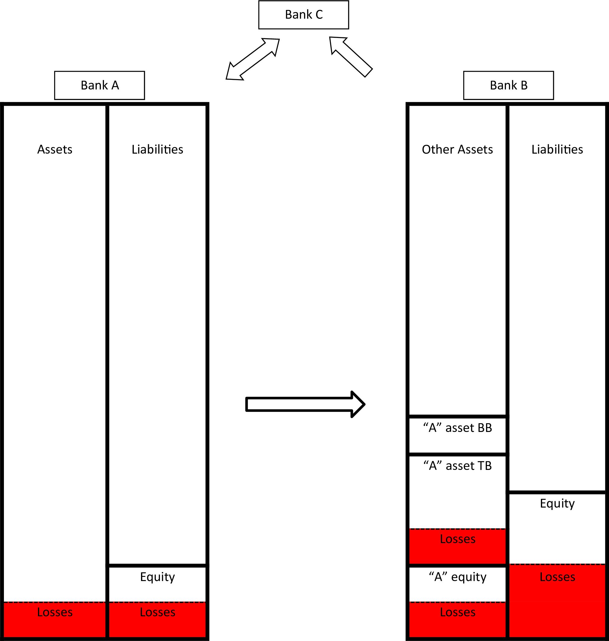
Figure 1 tries to explain the expected output of task 1. If bank A suffers a loss on its assets, the value of its equity reduces. This has an impact on bank B, but it is different for various instruments and for instruments in the “trading book” compared to instruments in the “banking book”. The same happens to the other banks that own instruments issued by bank A. Moreover, every bank hit by a loss has another impact on all the banks connected to it: the contagion is assessed with the simulation methodology developed in task 4. In case of bank default, this approach allows to determine the amount of the losses and, therefore, an endogenous RR for each instrument based on its seniority (for the Eurozone, also following the regulatory bail-in framework established by the “Single Resolution Mechanism”) and collateralization. Then, a real assessment of the asset side is not trivial, but is overly important.

Bank A suffers a loss. This causes losses to banks B and C. For instance, we assume (using only equity and “other assets” exposures) that it largely reduces the value of bank A’s equity held by bank B (“A” equity), reduces less the value of the “other assets” held by bank B in its trading book (“A” asset TB), and does not reduce the value of the “other assets” held by bank B in its banking book (“A” asset BB). The same happens in the balance sheets of bank C. Moreover, for example, the losses of bank B implies losses for bank C that owns instruments issued by B, while the losses of bank C implies further losses to bank A, as indicated by the arrows. The figure is purely schematic and is not intended to indicate the relative magnitudes of the various parts of the balance sheet.
3.4) Task 2 – Banks’ response to the crisis
In this task, the team should study the strategies that banks and other institutions can perform in order to rebalance their balance sheets, and to comply the regulatory constraints, in case of illiquidity and/or undercapitalization problems. As explained in Subsection 2.1, the full set of regulatory constraints have to be applied to really assess their situations and their (sometimes forced) behaviours.9 Fixing this set of constraints is relatively easy given that they are obtained by the financial regulation.
The team should then investigate the various strategies that FIs can theoretically implement. This task can be performed in various ways, indeed the team can:
find the optimal strategy in order to minimize losses;
analyze some case studies of FIs that rearrange their balance sheets after a crisis;
analyze (for banks) the strategies proposed in the recovery and resolution plans provided by the banking institutions. This procedure could present a huge number of different strategies. Therefore, the team should fix one or, at most, few possible strategies that could be applied to banks having different banking business models (that is, banks focused on traditional lending versus banks largely performing investment banking activities), or to banks clustered according to the main actions prearranged in their recovery and resolution plans.
These strategies will be applied to all the FIs including the one(s) that is assumed to suffer the initial shock. Indeed, the methodology can simulate both an initial liquidity shock (for instance, a reduction of deposits, such as a bank run, due to a risk aversion increase) and a solvency shock (for instance, a write-off or write-down of loans involving losses that reduce the equity value). Then, once the losses on various instruments for a given shock are determined, the surviving banks may again present the two problems already mentioned (illiquidity and/or undercapitalization).
An example of a general strategy for a bank facing a liquidity problem could be the following. After using cash and reserves, if it is an interbank lender, it can first stop the short term interbank loans. If this action is not enough or the bank is an interbank borrower, it should follow a strategy that reduces the losses, that is it can use in the following priority order: (i) central bank credit, provided it can pledge enough eligible securities (with an haircut), (ii) money from repos in the market against the marketable-but-not-eligible securities or from ABS backed by its loans (with haircuts respectively), (iii) money from fire sale of part of the remaining assets with a discount that can give rise to capital losses. If this is not sufficient, then the bank is not liquid enough to repay its exposure, a partial repayment occurs, and it is suspended by the authorities.
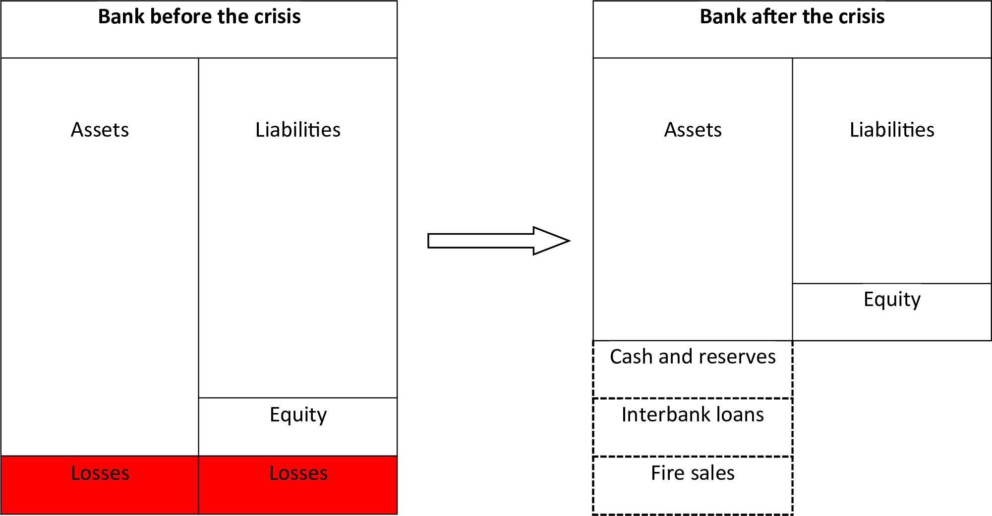
About solvency, instead, a bank that suffers losses can feature the undercapitalization problem. The undercapitalized bank, that cannot raise equity capital from the market in the very short run (especially during a systemic crisis), has to carry out the required deleveraging, that is it has to sell some assets to have money to liquidate its liabilities and to conform to minimum capital level and leverage ratio as set in the Basel III reform. Figure 2 shows that the reduced equity implies a smaller balance sheet. However, again, banks should follow a strategy to remove the assets that minimizes losses. For example, if the bank is an interbank lender, the first assets that it could try to dispose of are the short term interbank loans. Then, it may sell the most liquid assets and so on, till a fire sale of the remaining marketable assets at a discounted price that gives rise to capital losses. If this is not enough, it is classified as undercapitalized and subject to the liquidation procedure or the resolution tools and, in particular, to the bail-in procedure.

Undercapitalized banks have to sell some assets to deleverage in order to conform to regulatory constraints. Banks should follow a strategy in order to dispose of the assets that minimize the reduction of the return, in particular trying to avoid fire sales. The figure is purely schematic and is not intended to indicate the relative magnitudes of the various parts of the balance sheet.
Till now, I have tackled the issue of the behaviour of the FIs directly involved in the contagion process. However, the simulation should sketch the behaviour of non-FIs and of FIs not involved in the contagion, in order to account for liquidity hoarding and bank run mechanisms. For instance, if a regulatory ratio of a bank decreases below a certain threshold, the other banks that are interbank lenders can stop the short term interbank loans to that bank, and/or the depositors can perform a bank run. The money withdrawal could be modelled as a function of the gap between the actual value and the fixed threshold of a selected regulatory ratio, and as a function of the endogenous seriousness of the overall contagion: for instance, the model can simulate a freezing of the whole interbank market in the presence of a large contagion.
All in all, at the end of the simulation (and considering all the interactions among the explained mechanisms), the model will be able to determine illiquid and undercapitalized banks.
3.5) Task 3 – Fire sales estimates
Task 3 performs an econometric study of the price movements of financial instruments, not issued by FIs, in a fire sales context. In particular, the team should determine a price reaction function that will depend negatively (that is, it performs smaller price changes) on the liquidity of the instrument, and will depend positively (larger changes) on the amount sold endogenously determined in the simulation. Therefore, a simulation that involves a large crisis for the financial sector will be associated to stronger fire sales and to higher price drops of market instruments.
Moreover, the team should connect the price reaction function to a haircut reaction function because, as already explained, when market prices decline, the value of collateral decreases causing an increase of the “haircuts” applied to the collateral (Brunnermeier and Pedersen, 2009). It is very important because haircuts have to be applied in the various operations (central bank’s open market operations, repos, etc.).
Cifuentes et al. (2005) is an early example of a fire sale model. Nier et al. (2007) and Gai and Kapadia (2010) insert the fire sale model by Cifuentes et al. (2005) in their models of direct exposures. Montagna and Kok (2016) insert an endogenous price, function of the sold amount and of the depth of the market for that security, in the common exposures layer of their simulation. Two relevant recent models of fire sales are Greenwood et al. (2015) and Duarte and Eisenbach (2013, revised in 2018). These two models are based on the assumption of a leverage target, which leads to a linear deleveraging rule in reaction to a loss. This is an unreliable assumption in stress scenarios. Indeed, as explained by Cont and Schaanning (2017), “there is some empirical evidence that in the medium term large FIs maintain fairly stable levels of leverage - Adrian and Shin (2010) - but it is not clear why the same institutions would enforce such leverage targets in the short term, especially in stress scenarios where this could entail high liquidation costs”. They explain that deleveraging is the result of investor redemptions for funds, “but for regulated FIs such as banks, large scale deleveraging is mainly driven by portfolio constraints - capital, leverage or liquidity constraints - which may be breached when large losses occur”. Therefore, they develop a quantitative framework to model fire sales in a network of FIs with common asset holdings, subject to regulatory constraints (for simplicity, they focus only on leverage constraint). The paper Cont and Schaanning (2017) is a good starting point for this task.
In this task, the team should perform three jobs. The first is to choose which classes are relevant for the analysis of the contagion, analogously to the second job of the first task. In particular, Cont and Schaanning (2017) divide the assets held by each institution in two types: illiquid assets not subject to fire sales (including non-securitized loans, commercial and residential mortgage exposures, retail exposures, intangible assets…) and marketable securities, which may be liquidated over a short time scale if necessary (including sovereign bonds, corporate bonds and derivative exposures). In this way, they also consider the possibility of a default due to a liquidity problem; indeed, an institution could be solvent thanks to the presence of a large amount of illiquid assets, but could go bankrupt because of the illiquidity problem. This is very relevant because they “observe that, while insolvency is the dominant mode of failure of banks in scenarios associated with extremely large initial shocks, illiquidity is the dominant mode of failure in scenarios associated with moderate shocks which are nevertheless large enough to trigger fire sales”.
The marketable securities need to be further split into many categories characterized by a different market depth parameter, according to a different market liquidity level. This partitioning is, therefore, strictly related to the second job of this task, that is the estimation of a price reaction function. The team should econometrically study the time series of various market instruments with different degrees of liquidity, focusing especially on the recent worst market crashes. Therefore, there is the need to use market data (both prices and volumes). If the available datasets will not be large enough to generate reliable estimates, as a contingency plan, some event studies may be analysed. These analyses could also be performed starting from the vast market microstructure literature of pricing formation (for a recent literature review see, for instance, Barucci and Fontana, 2017, Chapter 10). This is probably the most difficult job of the whole methodology, because many features have to be considered. Firstly, the price change should be a function of the sales of the analysed asset, but also of the overall sales in the market, given that almost all price movements have an idiosyncratic component, but also a systematic component related to the whole market. The presence of the market component is very relevant and it is always neglected: in case of a market crash, all FIs could suffer losses on their “trading book”, even if they do not hold the assets that are fire sold. These widespread losses have to be accounted for. Secondly, the sequence of events is not simple: the amount needed to be fire sold can derive from the loss of the financial institution, but the loss derives from the fire sales and, moreover, the fire sold amount can be computed sequentially for each institution hit in the contagion, but it should consider the fact that the contagion could be simultaneous and feature reverberations among nodes. Thirdly, as explained by Cont and Schaanning (2017), the “implementation shortfall” has to be considered: assets are liquidated at price lowering during the fire sale process, with the first assets sold at the pre-fire sales prices and last assets sold at the post-fire sales prices. Therefore, the average selling price should stay in the middle between pre- and post-fire sales prices.
The team will then connect the price reaction function to a haircut reaction function. This job could be easier, given that it can also adopt regulatory guidelines (for instance, Covi et al., 2021, apply the ECB guideline).10
The third job is to decide the order in which the FIs sell their marketable assets. Greenwood et al. (2015), Duarte and Eisenbach (2013), and Cont and Schaanning (2017) assume that FIs sell their marketable assets proportionally. An alternative is to assume that FIs first sell the asset with the highest market liquidity and so on until the marketable asset with the lowest market liquidity. Intermediate possibilities between the two proposed alternatives could represent an attempt to maximize the expected liquidation value (indeed, the optimal solution requires that the marginal rate of loss should be the same for all the marketable assets. For instance, selling a large amount of a more liquid asset and a small amount of a less liquid asset could be better than selling only the more liquid asset for a huge amount). Some empirical studies on asset sales during market crashes are needed.
In order to reduce the “model risk” (and the consequence reliability of the overall methodology), the team has to implement some sensitivity analysis on the estimated price and haircut reaction functions, and on the liquidation order, to check if the simulation output is robust.
3.6) Task 4 – Simulation procedure and its applications
The team should develop the simulation procedure. This is “simply” the technical implementation of the modelling framework which emerges from the other tasks. Once the losses on the various instruments issued by the FIs are determined for a given initial shock (task 1), and the FIs strategies established (task 2), the team will simulate the propagation of the distress in the multi-layer network (task 1-2-3). Banks and other FIs (also belonging to the shadow banking system) are represented by nodes and the (direct and weighted) multi-layer network has a layer for each relevant kind of asset determined in task 1 and 3. Therefore, there are two types of layers, depending on the issuer of the asset, that is a FIs (task 1) or not (task 3). Indeed, the layers of assets issued by FIs are represented by square matrices, while the layers of assets issued by non-FIs are bipartite networks.11 However one network dimension is common to all layers (equal to the number of the analysed FIs).
The simulation of the contagion will consider both liquidity and solvency problems, and both defaulted and non-defaulted banks and, for defaulted banks, the procedure will follow either a liquidation or a bail-in procedure depending on bank size, and will endogenously determine the RR based on the computed losses.
Moreover, the team should overcome the DebtRank assumption that contagion cannot repeat an “edge” between two nodes to circumvent infinite reverberations. The model should consider reverberations until the variations are below a (small) threshold.
Finally, the simulation will be ready to be applied by financial regulators to compute the systemic importance and the contagion losses. Effectively, we will obtain an estimate of the fraction of the total economic value of the financial system in distress. This can be used for a systemic stress-test exercise. Indeed, the simulation can be used to answer many questions about the impact on the financial system of:
a loss of a percentage “α” of the net worth of a financial institution or of a group of banks/FIs (due, for instance, to a write-down of loans or other assets);
a macroeconomic/sectorial shock. For instance, the model will be able to simulate a write-off of a specific non-financial asset that many banks have in common, or can simulate a shock for a selected group of institutions tied to a specific area or economic sector.
This should be the base to compute the systemic risk contribution, given by the expected systemic loss obtained by setting a probability of occurrence of the possible scenarios. It will allow to rank banks following their systemic importance and to detect the SIFIs.
Moreover, the methodology can be applied for other purposes/in other scenarios. First, in the presence of an actual crisis, the financial regulator can simulate various strategies to reduce the consequences. Indeed, for each kind of shock (magnitude and nature), the proposed methodology will give the possibility to simulate and understand the most adequate macroprudential and microprudential response to avoid the contagion. This is a very hot topic for regulators, because they can implement several different strategies. For instance, Manna and Schiavone (2012) propose to compare costs and benefits of the following strategies: (i) widen the pool of assets accepted as collateral in monetary policy operations (with haircut) to all FIs; (ii) widen the pool of assets accepted as collateral in monetary policy operations (with haircut) to a few selected banks; (iii) ask for a compulsory bail-in of some creditors in the equity capital of few selected banks. Similarly, Covi et al. (2021) compute a “sacrifice ratio”, which measures the ratio of system-wide losses due to the failure of a bank over the cost of recapitalizing the bank by an amount equal to its capital requirements, in order to understand if a Government should perform a bail-out.
Second, this methodology can be used as an “Early Warning System”. Then, for instance, when the systemic losses due to some kind of shock or to the default of a bank go beyond a certain threshold, the regulators could ask for prudential regulation requests to prevent the crisis, such as an equity increase of some targeted banks (also determining the minimum capital growth needed).
Third, the simulation can help to improve the financial regulation, determining what happens in different scenarios with many interdependent regulatory rules. For instance, the Basel III agreement adds many other ratios (such as the liquidity coverage ratio or the leverage ratio) to the capital ratio. With the simulation, the financial regulator could understand if these rules reduce or enlarge the contagion in case of distress, and tune these constraints.
Fourth, starting from this analysis, the financial regulators will be able to obtain a further insight into the short run consequences on the real economy due to the simulated initial (real or financial) shock: knowing the overall equity loss of the financial system and, in particular, the loss of each major bank, the regulator could estimate the credit restriction to the real economy. In the words of Glasserman and Young (2016) “the level of connectivity between the financial and nonfinancial sectors (…) is extremely important in amplifying (or dissipating) shocks to the system”. A similar further step is already sketched in Huser and Kok (2020): they build the wider macro-financial network, where the Euro Area banking sector is connected to other Euro Area sectors via securities exposures, in order to investigate both the different sectoral funding and the different exposure patterns.
4) Conclusions
Reduction and management of the financial systemic risk is one of the most important regulatory topics, because of its enormous socio-economic impact. Indeed, a financial crisis can trigger a large and prolonged real economic crisis, as shown by the 2007-2008 crisis. Therefore, it is essential that monitoring authorities are able to measure the systemic risk and to identify which FIs are so important that their crisis can trigger a crisis of the whole financial system (that is, they are SIFIs).
The current proposal starts from the growing literature strand that performs agent-based simulation procedures of network contagion. Indeed, the network theory is probably the best tool for analysing the contagion risk, because the financial system is well suited for a representation in which nodes represent institutions and links represent financial relations. However, all the simulations proposed in the literature present some of the following shortcomings: (i) lack of a “real” balance sheet of the analysed FIs, (ii) lack of an endogenous price function for different kinds of instruments, (iii) lack of the impact of distressed, but non-defaulting, institutions, (iv) lack of the full set of regulatory constraints, (v) lack of a reliable reaction behaviour of all agents involved in the simulation. Moreover, the systemic risk assessment needs to consider the relevant exposures of all the relevant SIFIs (not only the G-SIBs), and to integrate the approach globally.
Therefore, an improved simulation is suggested to model the direct network contagion channel (interconnectedness of balance sheet of FIs, including direct losses and liquidity hoarding), also integrating the indirect contagion channel (fire sales and bank runs), in order to reach the full representation of the financial systemic risk.
This complex methodology can be built only by the financial regulators, to which this proposal is addressed. Indeed, there is the need to build a large team in order to integrate different research fields (in particular, econometrics, financial regulation, and network analysis), and the need to use supervisory datasets that are not publicly available.
Footnotes
1.
See the Appendix for a list of all acronyms used in the paper.
2.
FIs lend less than 100% of the price of the collateral and this reduction is called “haircut”.
3.
See, for instance, the papers of ECB staff such as, Covi et al. (2021); Hüser et al. (2018); Huser and Kok (2020); Montagna and Kok (2016).
4.
The trade-off between individual risk and systemic risk is present even in the fire sale context: studies, such as Cecchetti et al. (2016); Raffestin (2014); Wagner (2011), show that diversification is not always beneficial. Indeed, on one hand, a well-diversified portfolio allocation reduces the bankruptcy probability but, on the other hand, if many investors pursue the same strategy (that Fixing this set of constraints is a large diversification) then there is a strong risk of facing higher liquidation costs due to a joint liquidation event.
5.
Some papers focus on the network of exposures on derivatives, such as Bardoscia et al. (2019), and Paddrik et al. (2020).
6.
For instance, Hüser et al. (2018) used the 26 largest euro area banking groups for their analysis.
7.
As explained by Glasserman and Young (2015), the lack of information is a problem for regulators, but also for market participants. Indeed, the “lack of information is itself a contributor to contagion, and may lead to cascades and funding runs that would not occur if the network of obligations were known with greater certainty”.
8.
The SPPI test requires that the contractual terms of the financial asset give rise to cash flows that are solely payments of principal and interest on the principal amounts outstanding. Cash flows that provide compensation for risks such as equity or commodity risk will fail the SPPI test.
9.
A real behavioural assessment should consider the possibility for FIs to stipulate new contracts, that is adding new edges to the network. Therefore, a further analysis of the network dynamics could be performed. However, given that the proposed methodology is determined to simulate the very short run, and that in the presence of a large crisis the usual network dynamics are often frozen, adding debatable assumptions to consider this feature could only increase the “model risk”.
10.
11.
If, for some network analyses, there is the need of have the same structure in all layers, to obtain the corresponding square networks from the bipartite cases, the projected networks of common exposures can be built.
Appendix
Table of acronyms
| BB | Banking Book |
| DGI | G-20 Data Gaps Initiative |
| EA | Euro Area |
| ECB | European Central Bank |
| EMIR | European Market Infrastructure Regulation (EU Regulation 648/2012) |
| EU | European Union |
| FIs | Financial Institutions |
| FSB | Financial Stability Board |
| G-SIBs | Global Systemically Important Banks |
| IASB | International Accounting Standards Board |
| IFRS | International Financial Reporting Standards |
| IMF | International Monetary Fund |
| LGD | Loss Given Default |
| MiFID 2 | Markets in Financial Instruments Directive (EU Directive 65/2014) |
| MiFIR | Markets in Financial Instruments Regulation (EU Regulation 600/2014) |
| OFR | U.S. Office of Financial Research |
| PD | Probability of Default |
| RR | Recovery Rate |
| SIFIs | Systemically Important Financial Institutions |
| SPPI test | Solely Payments of Principal and Interest on the principal amount outstanding test |
| TB | Trading Book |
References
-
1
Capital Shortfall: A New Approach to Ranking and Regulating Systemic RisksAmerican Economic Review 102:59–64.https://doi.org/10.1257/aer.102.3.59
- 2
-
3
The Changing Nature of Financial Intermediation and the Financial Crisis of 2007–2009Annual Review of Economics 2:603–618.https://doi.org/10.1146/annurev.economics.102308.124420
-
4
Multiplex interbank networks and systemic importance: An application to European dataJournal of Financial Stability 35:17–37.https://doi.org/10.1016/j.jfs.2016.12.008
- 5
-
6
Multiplex network analysis of the UK over‐the‐counter derivatives marketInternational Journal of Finance & Economics 24:1520–1544.https://doi.org/10.1002/ijfe.1745
-
7
The multiplex structure of interbank networksQuantitative Finance 15:673–691.https://doi.org/10.1080/14697688.2014.968356
-
8
Network analysis and calibration of the “leveraged network-based financial accelerator.”Journal of Economic Behavior & Organization 99:109–125.https://doi.org/10.1016/j.jebo.2013.12.018
-
9
Network calibration and metamodeling of a financial accelerator agent based modelJournal of Economic Interaction and Coordination 15:413–440.https://doi.org/10.1007/s11403-018-0217-8
- 10
-
11
Leveraging the network: A stress-test framework based on DebtRankStatistics & Risk Modeling 33:117–138.https://doi.org/10.1515/strm-2015-0005
-
12
Liaisons dangereuses: Increasing connectivity, risk sharing, and systemic riskJournal of Economic Dynamics and Control 36:1121–1141.https://doi.org/10.1016/j.jedc.2012.04.001
-
13
DebtRank: too central to fail? Financial networks, the FED and systemic riskScientific Reports 2:541.https://doi.org/10.1038/srep00541
-
14
Where the Risks Lie: A Survey on Systemic Risk*Review of Finance 21:109–152.https://doi.org/10.1093/rof/rfw026
-
15
A Survey of Systemic Risk AnalyticsAnnual Review of Financial Economics 4:255–296.https://doi.org/10.1146/annurev-financial-110311-101754
-
16
Looking deeper, seeing more: A multilayer map of the financial systemOffice of Financial Research Brief 16:06–12.
-
17
Systemic risk measurement: bucketing global systemically important banksAnnals of Finance 17:319–351.https://doi.org/10.1007/s10436-021-00391-7
-
18
SRISK: A Conditional Capital Shortfall Measure of Systemic RiskReview of Financial Studies 30:48–79.https://doi.org/10.1093/rfs/hhw060
-
19
Recovery rates, default probabilities, and the credit cycleJournal of Banking & Finance 34:754–764.https://doi.org/10.1016/j.jbankfin.2009.04.009
-
20
Market Liquidity and Funding LiquidityReview of Financial Studies 22:2201–2238.https://doi.org/10.1093/rfs/hhn098
-
21
Oxford Handbook on the Economics of Networks306–326, Financial contagion in networks, Oxford Handbook on the Economics of Networks, Oxford University Press, p.
-
22
Contagion and Fire Sales in Banking NetworksSSRN Electronic Journal pp. 1–72.https://doi.org/10.2139/ssrn.2757615
-
23
Fire sales and the financial acceleratorJournal of Monetary Economics 59:336–351.https://doi.org/10.1016/j.jmoneco.2012.04.001
-
24
Liquidity Risk and ContagionJournal of the European Economic Association 3:556–566.https://doi.org/10.1162/jeea.2005.3.2-3.556
-
25
Lending relationships in the interbank marketJournal of Financial Intermediation 18:24–48.https://doi.org/10.1016/j.jfi.2008.06.003
-
26
Handbook of Systemic Risk327–368, Network Structure and Systemic Risk in Banking Systems, Handbook of Systemic Risk, Cambridge University Press, p.
-
27
Fire Sales, Indirect Contagion and Systemic Stress TestingSSRN Electronic Journal pp. 1–50.https://doi.org/10.2139/ssrn.2955646
-
28
CoMap: Mapping Contagion in the Euro Area Banking SectorJournal of Financial Stability 53:100814.https://doi.org/10.1016/j.jfs.2020.100814
-
29
Model risk of risk modelsJournal of Financial Stability 23:79–91.https://doi.org/10.1016/j.jfs.2016.02.002
- 30
-
31
An Analysis of the Japanese Credit NetworkEvolutionary and Institutional Economics Review 7:209–232.https://doi.org/10.14441/eier.7.209
-
32
Indicators to Support Monetary and Financial Stability Analysis: Data Sources and Statistical Methodologies1–23, Capital and Contagion in Financial Networks, IFC Bulletins Chapters, in: Bank for International Settlements (Ed), Indicators to Support Monetary and Financial Stability Analysis: Data Sources and Statistical Methodologies, Vol, 39, p.
-
33
Complexity, concentration and contagionJournal of Monetary Economics 58:453–470.https://doi.org/10.1016/j.jmoneco.2011.05.005
-
34
Contagion in financial networksProceedings of the Royal Society A 466:2401–2423.https://doi.org/10.1098/rspa.2009.0410
-
35
How likely is contagion in financial networks?Journal of Banking & Finance 50:383–399.https://doi.org/10.1016/j.jbankfin.2014.02.006
-
36
Contagion in Financial NetworksJournal of Economic Literature 54:779–831.https://doi.org/10.1257/jel.20151228
-
37
Vulnerable banksJournal of Financial Economics 115:471–485.https://doi.org/10.1016/j.jfineco.2014.11.006
-
38
Ranking consistency of systemic risk measures: a simulation-based analysis in a banking network modelReview of Quantitative Finance and Accounting 52:953–990.https://doi.org/10.1007/s11156-018-0732-7
-
39
Challenges in identifying and measuring systemic riskRisk Topography: Systemic Risk and Macro Modeling, NBER Conference Report. pp. 15–30.
-
40
Too interconnected to fail: A survey of the interbank networks literatureThe Journal of Network Theory in Finance 1:1–50.https://doi.org/10.21314/JNTF.2015.001
-
41
The systemic implications of bail-in: A multi-layered network approachJournal of Financial Stability 38:81–97.https://doi.org/10.1016/j.jfs.2017.12.001
-
42
Mapping bank securities across euro area sectors: comparing funding and exposure networksThe Journal of Network Theory in Finance 5:59–92.https://doi.org/10.21314/JNTF.2019.052
-
43
Second Phase of the G-20 Data Gaps Initiative (DGI-21–15, Second Phase of the G-20 Data Gaps Initiative (DGI-2, Third Progress Report, p.
-
44
https://www.sec.gov/files/US-Credit-Markets_COVID-19_Report.pdfhttps://www.sec.gov/files/US-Credit-Markets_COVID-19_Report.pdf.
-
45
Robustness and informativeness of systemic risk measures, Deutsche Bundesbank1–50, Discussion Paper n.04/2013, 10.2139/ssrn.2796895.
-
46
Externalities in Interbank Network: Results from a Dynamic Simulation ModelSSRN Electronic Journal pp. 1–40.https://doi.org/10.2139/ssrn.2207918
-
47
A multiplex network analysis of the Mexican banking system: link persistence, overlap and waiting timesThe Journal of Network Theory in Finance 1:99–138.https://doi.org/10.21314/JNTF.2015.006
-
48
Multi-Layered Interbank Model For Assessing Systemic RiskSSRN Electronic Journal pp. 1–55.https://doi.org/10.2139/ssrn.2830546
-
49
A survey of network-based analysis and systemic risk measurementJournal of Economic Interaction and Coordination 13:241–281.https://doi.org/10.1007/s11403-016-0182-z
-
50
Network models and financial stabilityJournal of Economic Dynamics and Control 31:2033–2060.https://doi.org/10.1016/j.jedc.2007.01.014
-
51
The information in systemic risk rankingsJournal of Empirical Finance 38:461–475.https://doi.org/10.1016/j.jempfin.2016.01.002
-
52
Contagion in Derivatives MarketsManagement Science 66:3603–3616.https://doi.org/10.1287/mnsc.2019.3354
-
53
The multi-layer network nature of systemic risk and its implications for the costs of financial crisesJournal of Financial Stability 20:70–81.https://doi.org/10.1016/j.jfs.2015.08.001
-
54
Diversification and systemic riskJournal of Banking & Finance 46:85–106.https://doi.org/10.1016/j.jbankfin.2014.05.014
-
55
Reconstructing and stress testing credit networksJournal of Economic Dynamics and Control 111:103817.https://doi.org/10.1016/j.jedc.2019.103817
-
56
Unstable bankingJournal of Financial Economics 97:306–318.https://doi.org/10.1016/j.jfineco.2009.10.007
-
57
An analysis of the literature on systemic financial risk: A surveyJournal of Financial Stability 28:91–114.https://doi.org/10.1016/j.jfs.2016.12.004
-
58
Systemic Liquidation Risk and the Diversity-Diversification Trade-OffThe Journal of Finance 66:1141–1175.https://doi.org/10.1111/j.1540-6261.2011.01666.x
Article and author information
Author details
Funding
No specific funding for this article is reported.
Acknowledgements
I am grateful for helpful comments and useful suggestions to participants in the "WEHIA October Workshop" (organized online by Università Cattolica di Milano, October 15th 2021), and in the 4th International Workshop on "Financial Markets and Nonlinear Dynamics - FMND" (Paris, May 31st - June 1st 2019).
Publication history
- Version of Record published: August 31, 2022 (version 1)
Copyright
© 2022, Riccetti
This article is distributed under the terms of the Creative Commons Attribution License, which permits unrestricted use and redistribution provided that the original author and source are credited.