Sequential macro-micro modelling with behavioural microsimulations

Cite this article as: J. Lay; 2010; Sequential macro-micro modelling with behavioural microsimulations; International Journal of Microsimulation; 3(1); 24-34. doi: 10.34196/ijm.00022

Article
Figures and data
Jump to

Abstract

This paper presents a sequential methodology that combines a macroeconomic CGE model with a behavioural microsimulation, illustrates the approach with applications, and discusses its merits and shortcomings. The microsimulation, based on a household income generation model, allows for incorporating individual fixed effects into macro-micro analysis. We argue that one of the main merits of the sequential approach is its flexibility. However, this flexibility comes at the cost of theoretical inconsistency.

Introduction

Analyzing the poverty and distributional impact of macro events requires understanding how shocks or policy changes on the macro level affect household income and consumption. It is clear that this poses a formidable task, which of course raises the question of the appropriate methodology to address such questions. This paper presents one possible approach: A sequential methodology that combines a macroeconomic model with a behavioural microsimulation. We discuss the merits and shortcomings of this approach with a focus on developing country applications with a short to medium run time horizon.¹

Most analyses of the poverty and distributional impact of macro shocks have turned to Computable General Equilibrium (CGE) models, which typically incorporate different representative household groups with a given within-group income distribution. Yet, recent empirical findings on distributional change indicate that changes within household groups distributions account for an important share of overall distributional change (Bourguignon et al., 2005b). At first sight, an obvious solution to this problem seems to increase the number of household groups, or even to incorporate all households from representative household surveys into the CGE model. Similarly – yet without providing heterogeneous feedback into the CGE model – micro-accounting techniques on the basis of household survey data that apply changes in factor prices at the individual level using household survey-data could be used to increase household heterogeneity. In an assessment of Russia’s accession to the World Trade Organization (WTO), Harrison et al. (2000) however find differences in poverty and distributional outcomes between a model with 10 representative household groups and a model with 55 000 households to be negligible.

Such evidence does not imply that household heterogeneity would not matter for a true understanding of the poverty and distributional impacts of macroeconomic shocks. It merely shows that even full heterogeneity of households in terms of factor endowments and consumption patterns does not make a difference in a standard CGE model. Microeconomic evidence on the drivers of changes in income distributions however suggests that applied CGE models (including those combined with household-survey-based micro-accounting models) may fail for a different reason: The importance of individual heterogeneity and decisions taken at the individual level for distributional and poverty outcomes; in other words, the importance of “individual behavior”. On the labor market, individual decisions include entry into the labor market, falling into unemployment or switching between sectors or occupations. Of course, CGE models can be extended to include for example unemployment and/or endogenous labor supply. Yet, in order to capture the income distribution implications, decisions would have to taken by “real” individual household members. This implies to introduce individual “fixed effects” and eventually requires the estimation of structural labor market models (Bourguignon et al., 2005a) that would need to be integrated in a general equilibrium framework. The estimation of such structural labor market models is by no means a trivial exercise and embedding them into a general equilibrium framework an additional challenge.²

This paper presents a less ambitious and more pragmatic approach. The sequential macro-micro approach that links a macroeconomic model, for example an applied CGE model, to a behavioural microsimulation model has two distinguishing features. First, it is sequential. A counterfactual scenario is generated in the macro (CGE) model. Then specific poverty and distribution-relevant link variables, for example wages and employment, are passed to a microsimulation model. Second, the microsimulation has behavioural components. For the microsimulation, individual and household decisions are modeled using microeconometric techniques on household and employment survey data. Through the microsimulation, the combined model hence incorporates individual “fixed effects” into the analysis.

The paper is structured as follows. We first outline some important characteristics of macro models used as part of a sequential model and present a stylized specification of a labor market that produces the link variables for our illustrative macro-micro model. We then provide a simple representation of household income generation that forms the core of the of our prototype behavioural microsimulation. We describe the simulation mechanics of the micro model. The next section presents two applications of this approach before we assess its strengths, weaknesses, and challenges. The final section concludes.

A stylized macro-micro model with a behavioural microsimulation

The macro model and the link variables

The sequential approach presented in this paper requires a macro model that produces changes in distribution and poverty-relevant (aggregate) variables that are passed to a microsimulation model. These variables, which we label “link variables”, are prices and quantities on factor and goods markets. Link variables from factor markets include real wages for different types of labor, returns to land and different types of capital. Factor quantities, for example the sectoral composition of labor, may also be passed from a macro model to a microsimulation. Finally, goods prices and quantities may operate as link variables. The developing country applications presented in this paper use applied trade-focused CGE models.³ Yet, other types of macro models with very different foci and features, including other forms of general equilibrium models (real business cycle models, and stochastic dynamic general equilibrium models) and macroeconometric models, may be more suitable in different contexts and for different questions. The illustrative framework presented in the following is general enough to allow the reader to imagine the application of a sequential macro-micro approach using very different models both at the macro and micro level, and different link variables.

If a macro model is built as part of a sequential macro-micro model, its labor market specification is the key component and will have to be compatible with the microsimulation model that we present below. The following representation of a labor market should be thought of as being embedded, for example, in an applied multisectoral CGE model that distinguishes between formal and informal production sectors. The associated labor markets are assumed to exhibit structural imperfections with different clearing mechanisms for these sectors. For the simplicity of exposition, we abstract from other factors of production and assume that the formal and informal sector produce the same good. Let total employment be fixed and assume that factors are fully employed. Hence, total employment will be the sum of formal and informal employment: L = L^f + L^if.

In a simple neoclassical world with full mobility of labor between formal and informal sectors, wages in the formal and informal sectors, which produce with different technologies will be the same:

(f_{f} (L^{f}), f_{i f} (L^{i f})) \cdot

Employment in formal and informal sector, respectively, and hence the formal labor share in this economy will be determined by the equation of marginal labor products in formal and informal sectors, as expressed in Equation (2).

\frac{W^{f}}{p} = \frac{W^{i f}}{p} = f_{f}^{'} (L^{f}) = f_{i f}^{'} (L^{i f})

Now assume that different wage setting mechanisms exist: In the formal sector, wages are rigid, for example due to the presence of bargaining by trade unions or efficiency wages. This rigidity can be represented by a “wage curve”, as in Equation (3) where the real formal sector wage becomes a function of the ratio of formal to informal employment.

\frac{w^{f}}{p} = g (\frac{L^{f}}{L - L^{f}})

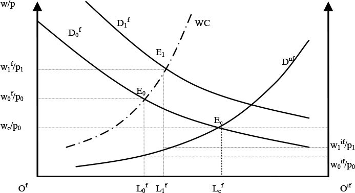
Without unemployment, the informal sector will now absorb the remaining workforce and the informal sector wage will adjust such that labor demand by the informal sector equals “residual” labor supply. This is depicted in Figure 1, where E_c illustrates the competitive equilibrium and w_c/p₀ the corresponding wage. With WC, the wage curve, the equilibrium wage and employment levels are represented by E₀. The formal sector wage w₀^f/p₀ will now be higher than the informal sector wage w₀^if/p₀. Accordingly, formal sector employment L₀^f will be lower than in the competitive case L_c^f.

Figure 1

Download asset Open asset

Formal and informal labor markets.

*Source*: Author’s compilation.

Real wages and employment in formal and informal sector, respectively, constitute the link variables in our illustrative macro-micro model:

\frac{w^{f}}{p}, \frac{w^{i f}}{p}, L^{f}, L^{i f} .

We now consider a policy experiment that shifts formal labor demand and leads to a new equilibrium in E₁. The formal sector wage increases to w ^f/p₁ and formal employment to L₁^f. The informal sector wage will increase as well from w₀^if/p₀ to w₁^if/p₁. Hence, the counterfactual values for our link variables⁴ that will be passed to the microsimulation will be

\frac{w_{1}^{f}}{p_{1}}, \frac{w_{1}^{i f}}{p_{1}}, L_{1}^{f}, L_{1}^{i f} \cdot

A prototype income generation model: The microsimulation

This section describes a prototype microsimulation model that can be used in combination with above CGE model to simulate the poverty and distributional impacts of shocks. The basis of the microsimulation is a household income generation model that needs to be compatible with the above CGE model. For good reasons, we avoid the term consistency here and refer to compatibility instead, as the macro and micro models will not be strictly consistent, neither theoretically nor empirically. We will return to this very important issue in more detail later. The household income generation model is estimated from household survey data with individual-level employment information.

In the microsimulation, we hence model the household income generation process.⁵ This implies that individuals make occupational choices and earn wages or profits accordingly. These labor i 1 market incomes plus exogenous other incomes, such as transfers and imputed housing rents, comprise household income. The components of the income generation model are thus an occupational choice and an earnings model. In the choice model, individual agents can choose between wage-employment and self-employment.⁶ We thus ignore labor market participation choice in this illustrative model. The occupational choice model is assumed to be slightly different for household heads other household members. Once occupational choices are made, earnings are generated accordingly either in the form of wages or as profits for the self-employed. Being self-employed means being part of what might be called a “household-enterprise”, in which all self-employed members of a household pool their incomes. The wage-employment market is segmented: the wage setting mechanisms are assumed to differ for skilled and unskilled labor as well as for females and males, which implies that there are four wage labor market segments.

The following set of equations describes the household income generation model. Household income Y_hh is earned by k_hh members, who are (and remain) active on the labor market (Equation 3 below). They are active either in the formal (with DF_i = 1, a dummy variable for formal sector employment) or informal sector (DF_i – 1(−1) = 1 if DF_i = 0) and earn the corresponding wages w_i, w_i^if. In addition, the household receives an exogenous nominal income ¯y_hh, for example transfers or remittances. All these components are real values, i.e. deflated with prices p. In practice, p will be assumed to be one in the initial situation. Per capital income y_hh is obtained by dividing household income by household size (Y_hh / hsize) so that (y₁,y₂,…,y_n) denotes the distribution of income when each observation is weighted with household size.

Y_{h h} = \frac{1}{p} \sum_{i = 1}^{k_{h h}} (w_{i}^{f} D F_{i} + w_{i}^{i f} (D F_{i} - 1) (- 1) + {\bar{y}}_{h h})

Individual occupational choices – between informal and formal activities – can be described by the following functions, which are assumed to be different for household heads (h) and other household members (o). We suppress the individual index here. Equation (7) shows that the household head’s probability of being employed in the formal sector is a function of a linear expression with a constant term c^h and personal and household characteristics X^h, which can include for example education, age, and households composition variables.

P (D F^{h} = 1 | X^{h}) = g^{h} (c^{h} + X^{h} α^{h})

The choices of other household members are assumed to depend not only on their own individual characteristics X^o, but also on the household head’s occupational choice:

P (D F^{o} = 1 | X^{o}, D F^{h}) = g (c^{o} + X^{o} α^{o} + γ^{o} D F^{h})

Equations (9) and (7) express wages w in the formal (f) and informal (if) sectors, respectively, in log-linear form with X, a vector of personal characteristics, and u, a random error.

In \frac{w^{f}}{p} = c^{f} + X β^{f} + u^{f}

In \frac{w^{i f}}{p} = c^{i f} + X β^{i f} + u^{i f}

The model just described gives the household income as a non-linear function of observed and unobserved individual and household characteristics. This function depends on two sets of parameters, which include the parameters of the wage equations for informal and formal activities and the parameters in the utility associated with different occupational choices for household heads and other family members. The occupational choice equations as well as the corresponding wage equations can be estimated from standard household survey data. Estimating Equations (7) and (8) using discrete choice models (with dichotomous choices hence logit or probit models) and (9) and (10) using OLS (or other adequate estimation techniques⁷) yields the following parameter vector:

({\hat{c}}^{h}, {\hat{α}}^{h}, {\hat{c}}^{o}, {\hat{α}}^{o}, γ^{o}, {\hat{c}}^{f}, {\hat{β}}^{f}, {\hat{c}}^{i f}, {\hat{β}}^{i f}) .

In addition, we obtain ${\hat{u}}^{f}$ and ${\hat{u}}^{i f}$ as observed residuals from the wage equations. However, we only observe formal wages for individuals employed in the formal sector. As the microsimulation will allow individuals to switch between formal and informal activities, we simulate a residual for the non-observed wage, here by a random draw from a normal distribution with the respective (formal or informal) observed variance.⁸ We face a similar problem in the latent utility models necessary to estimate Equations (7) and (8). In these models, residuals cannot be observed and are hence generated from the distribution underlying the respective model, here either a normal (probit) or logistic (logit) distribution. Residuals have to be drawn consistent with the observed occupational choice, i.e. the utility an observed formal wage earner relates to formal employment has to be higher than the utility associated with informal employment. Statistically, this implies to draw these residuals conditional on the observed choice. These simulated residuals are denoted u1_i and u0_i. With ind, an indicator function that assumes a value of 1 (0) if the condition in brackets is (not) fulfilled, we thus have

D F_{i}^{h} = i n d ({\hat{c}}^{h} + X_{i}^{h} {\hat{α}}^{h} + u 1_{i} > u 0_{i})

and

D F_{i}^{o} = i n d ({\hat{c}}^{o} + X_{i}^{o} {\hat{α}}^{o} + γ^{o} D F^{h} + u 1_{i} > u 0_{i}) .

Here DF_i^h and DF_i^o will hence assume their observed values. This implies that the sum of these two dummies – defined either for household heads or other household members – over all individuals will give the total number formal sector employees L₀^f, consistent with the initial value of this link variable from the macro model. This is illustrated in Equation (14).

L_{0}^{f} = \sum_{h h} \sum_{i}^{k_{h h}} (D F_{i}^{h} \otimes D F_{i}^{o})

Accordingly, average wages in the formal sector can be expressed as follows:

\frac{w_{0}^{f}}{p} = \frac{\sum_{h h} \sum_{i}^{k_{h h}} [(D F_{i}^{h} \otimes D F_{i}^{o}) \cdot exp ({\hat{c}}^{f} + X_{i} {\hat{β}}^{f} + {\hat{u}}_{i}^{f})]}{L_{0}^{f}}

Similar expressions can be written down for informal sector employment and the corresponding wage, such that we can replicate all link variables in the initial equilibrium w₀^f,w₀^if,L₀^f,L ^if. Remember that this replication is based on the observed characteristics of the individuals (all X), unobserved and partially simulated characteristics (all u), and the estimated parameters.

Based on this micro replication of the initial situation, we can now micro-simulate the distributional and poverty implications of the changes in the link variables given by the macro model. In the simulation, the link variables

\frac{w_{1}^{f}}{p_{1}}, \frac{w_{1}^{i f}}{p_{1}}, L_{1}^{f}, L_{1}^{i f}

will hence be used as target values. This implies that individual earnings and occupational choices have to change such that they reproduce these targets on the aggregate level. There are a number of ways how this can be achieved. Obviously, the required individual changes in occupational choices can be obtained by varying the coefficients or the observed or unobserved individual characteristics. A typical choice in applied microsimulation models is to vary the constant(s). Hence, the chosen parameters are adjusted and occupational choices change accordingly, until the results of the microsimulation are consistent, at an aggregate level, with the given aggregates. Formally, the following constraint describes the consistency requirement where c₁^h is the constant in the heads’ occupational choice equation that is consistent with L₁^f.

L_{1}^{f} = \sum_{h h} \sum_{i}^{k_{h h}} [{(i n d (c_{1}^{h} + X_{i}^{h} {\hat{α}}^{h} + u 1_{i} > u 0_{i})} \otimes {i n d ({\hat{c}}^{o} + X_{i}^{o} {\hat{α}}^{o} + γ^{o} D F_{1}^{h} + u 1_{i} > u 0_{i})}]

Varying only the constant ${\hat{c}}^{h}$ (to c₁^h)implies that we assume that the macro shock only induces household heads to switch occupation. Other household members’ occupational choices are only affected through the possible change in the head’s occupational choice, i.e. in the case of DF₁^h ≠ DF^h. As this kind of behavior may not be realistic, we can alternatively assume that the constants of both the heads and other household members vary. However, without an additional restriction, changes in the two constants cannot be uniquely determined. A possible solution is to add a variable Δ to the constant term. In practice – when such equations are solved for real households from a household survey – we will typically be able to find a unique solution for Δ in Equation (18).

L_{1}^{f} = \sum_{h h} \sum_{i}^{k_{h h}} [A \otimes B]

where

A = i n d {({\hat{c}}^{h} + Δ) + X_{i}^{h} {\hat{α}}^{h} + u 1_{i} > u 0_{i}}

B = i n d {({\hat{c}}^{o} + Δ) + X_{i}^{o} {\hat{α}}^{o} + γ^{o} D F_{1}^{h} + u 1_{i} > u 0_{i}}

Using either approach to adjust the constant (or both constants) in the occupational choices, will thus enable us to replicate the changes in formal as well as formal employment given by the CGE model. Our very simple income generation model allows us to proceed step-wise. We first solve for changes in occupational choices, and simulate wages in the next step. The reason is that wages do not enter the occupational choices of individuals, as they might in a more complex – or structural – income generation model. However, changes in occupational choices enter the equation for aggregate wages, as the (observed and unobserved) characteristics of the individuals in the respective sectors change. As in the case of occupational choices, we can vary the constants in the respective sectors to equate wages given by the CGE model and those in the microsimulation.⁹ For the formal sector, this requires Equation (19) to hold with c₁^f, the new formal sector wage equation constant.

\frac{w_{1}^{f}}{p_{1}} = \frac{\sum_{h h} \sum_{i}^{k_{h h}} [(D F_{1 i}^{h} \otimes D F_{1 i}^{o}) . exp (c_{1}^{f} + X_{i} {\hat{β}}^{f} + {\hat{u}}_{i}^{f})]}{L_{1}^{f}}

The equation for the average informal sector wage can be derived accordingly. The solutions for the constants in the choice Equation (18) and the wage Equation (19) can be obtained using numerical solution algorithms, for example Gauss-Newton techniques. With counterfactual occupational choices and corresponding wages DF₁,w₁, we can now compute the counterfactual household income Y1_hh, as illustrated in Equation (20). We assume that exogenous transfers ¯y_hh are constant in nominal terms.

Y_{1 h h} = \frac{1}{p_{1}} \sum_{i = 1}^{k_{h h}} (w_{1 i}^{f} D F_{1 i} + w_{1 i}^{f} (D F_{1 i} - 1) (- 1) + {\bar{y}}_{h h})

with

D F_{1} = D F_{1 i}^{h} \otimes D F_{1 i}^{o}

With constant household size these counterfactual household incomes now yield a counterfactual income distribution that can be described by (y₁₁,y₁₂,…,y_1n).

Applications

The above prototype macro-micro model is intended to provide an introduction into the basic mechanics of a macro-micro model with a behavioural microsimulation. Which macro model to choose and which transmission channels to highlight eventually depends on the research or policy question and the context, in which it is placed. The two applications that we present in the following are based on recursive-dynamic, trade-focused national CGE models.¹⁰ The first application examines the possible poverty impacts of a Doha round scenario of further multilateral trade negotiations for the case of Brazil. The second assesses the poverty and distributional implications of the Bolivian gas shock.

As in the above model and most developing country applications, the focus is on the labor market, as reflected by the link variables that include average wages in different labor market segments, employment levels and the occupational composition of employment. The respective specification of the labor market represents the transmission channels considered to be of particular relevance for the policy and shock under consideration. The Brazilian model focuses on movements between agricultural and non-agricultural sectors, while the Bolivian model concentrates on formal-informal segmentation in the urban labor market. In both applications, the labor market is further segmented along skill levels.

The microsimulation models used in the subsequent applications share the reduced-form character of the above prototype model. Employment volumes in the respective labor market segments, for example unskilled agricultural employment, and wages are adjusted according to the results from the macro model. These adjustments are not triggered by individual responses to prices, for example relative wages – as they would in a (more) structural labor market model. As above, adjustments are obtained by changing the parameters of the estimated household income generation model.

The poverty impacts of trade liberalization in Brazil

Using this type of sequential model, Bussolo et al. (2006) ex-ante assess the poverty and distributional impacts of different uni- and multilateral trade liberalization scenarios for Brazil.¹¹ The labor market specification of the CGE model distinguishes between skilled and unskilled labor. While skilled workers are fully mobile across sectors, the labor market for the unskilled is segmented between agriculture and non-agriculture. This dual labor market for unskilled workers is modeled following a simple Harris-Todaro specification where the decision to migrate is a function of expected income in the non-agricultural sectors relative to the expected income in the agricultural sectors.

The micro model is linked to the macro model through changes in the following set of variables: First, changes in agricultural and non-agricultural labor income of unskilled labor; second, changes in labor income of skilled labor; third, changes in the sectoral (agriculture vs. non-agriculture) composition of the unskilled workforce. In addition, the microsimulation takes into account that unskilled and skilled labor supplies grow at different rates. These rates – also assumed to be exogenous in the CGE model – are derived from past trends of labor supply growth in the respective categories.

In accordance with the structure of the CGE model, the micro model thus simulates the decision to move from agriculture into non-agricultural sectors (or vice versa) only for unskilled workers. This simulation is based on a sectoral mover-stayer model that is estimated for heads and non-heads separately – as in the above prototype model. For this estimation, Bussolo et al. (2006) make use of a distinguishing feature of the PNAD¹². In contrast to many other household surveys, the PNAD provides information on employment histories, which allows the authors to identify movers between sectors and their characteristics at the time of moving. These characteristics include the type of land right the movers held or whether they were self-employed before they moved out of agriculture. These characteristics enter as explanatory variables into the mover-stayer model. As in the prototype model, the household income generation model is completed by Mincer-type wage equations for unskilled labor in agriculture and non-agriculture as well as for skilled labor. Individual labor incomes are aggregated as described above.

The mover-stayer model can be used to illustrate the behavioural content of the microsimulation model. For example, Bussolo et al. (2006) find a strong negative influence of own landholdings on the propensity to move. In contrast, higher educational achievements are making individuals more likely to move into non-agricultural employment. In addition, occupational choices of members of the same household are strongly correlated. In the simulation, individuals with no landholdings, better education and – in case of non-household heads – and moving household heads will hence be the first ones to move from agriculture into non-agricultural employment. Which individuals (landless, but better educated) move first, can make a difference in distributional outcomes. The movers’ characteristics will determine the composition of those who remain in agriculture (more with own landholdings, but less educated) as well the earning prospects in the non-agricultural sector (ceteris paribus better with better education).

With these components, the microsimulation involves two steps: First, unskilled labor moves out of agriculture until the new share of unskilled labor in agriculture given by the CGE is reproduced. Second, wages/profits are adjusted according to the CGE results taking into account the sectoral movements of unskilled labor from agriculture into non-agricultural sectors. Adjustments are achieved through the same procedures as in the above prototype model, i.e. the computation of new constants in the choice and wage equations, respectively, using numerical solution algorithms.

The analysis suggests that the economic effects of multilateral liberalization are rather limited for Brazil. Accordingly, poverty would remain largely unaffected by such reforms. In contrast, a full liberalization scenario implies quite substantial welfare gains that are concentrated among some of the poorest groups of the country, in particular those in agriculture. This scenario is also most interesting from a methodological viewpoint, as it highlights the benefits of a behavioural microsimulation. Under full liberalization, the rural poor benefit more than proportionately, a result driven – on the macro level – by an export boom in agriculture and agricultural processing industries, growing labor demand and associated higher wages. However, following full liberalization, a larger number of workers remain in agriculture compared to the baseline scenario. Given that moving out of agriculture may substantially improve the income situation of a household, one may expect full liberalization to weaken poverty reduction, an expectation supported by the observation that moving households are on average poorer than those remaining in agriculture (for example because they are landless). However, this is not the case, as the gain in agricultural incomes more than compensates the reduced benefits from lower migration flows (for example because they are better educated than those who stay in agriculture).

The poverty impacts of the Bolivian gas boom

Lay et al. (2008) examine the poverty effects of the gas boom Bolivia experienced in the late 1990s and early 2000s. Their analysis attempts to disentangle the effects of the resource-boom/bust from other shocks that the Bolivian economy experienced at the same time. The market for unskilled labor is segmented between rural and urban areas. The two segments are linked through rural-urban migration, modeled as in the Brazilian case as a function of the corresponding wage differential. In contrast, skilled labor is assumed to be fully mobile across all production sectors. Within the urban economy, unskilled workers are mobile between formal and informal sectors, but wage differentials observed in the base period are assumed to persist. These differentials point to systematically lower labor productivity in informal sectors.

Almost as in the prototype model, the macro model is linked to the microsimulation through the following set of variables: (1) the share of unskilled workers in the formal sector, (2) the share of skilled workers in the formal sector, (3) mean wages for skilled workers, (4) mean wages for unskilled workers, and (5) mean informal profits.¹³ Informal profits are understood as mixed income received by self-employed workers. Accordingly, they are calculated as the sum of skilled and unskilled labor income as well as informal capital income.

The two basic components of the income generation model in the Bolivian application are again a model of occupational choices that represents the choice between formal and informal employment as well as earnings functions that correspond to the respective sector of employment. Employment is assumed to be informal if the individual is self-employed/non-remunerated household member and/or works in an enterprise with less than 5 employees. If individuals happen to be in (or switch to) the formal sector they are assumed to earn a wage, whereas individuals in the informal sector are assumed to be (or become) part of a household enterprise and contribute to the profits earned by this enterprise. The choice between informal and formal activities is modeled separately for household heads, spouses, and other household members. In contrast to the above specifications, the equations of the choice model are interrelated through the head’s wage (and choice) that enters the occupational choice model of spouses and other household members. Again, occupational choices are hence assumed to be sequential with the household head deciding first. In line with the CGE model, the microsimulation distinguishes between unskilled and skilled labor. Separate wage equations for skilled and unskilled labor, respectively, hence describe earnings for individuals employed in the formal sector.¹⁴ The microsimulation again adjusts the constants to produce counterfactual occupational choices, earnings, and, eventually, household incomes and the corresponding distribution of income.

As in the Brazilian case, the microsimulation reveals the importance of individual characteristics that determine the sign and the strength of distributional change. Lay et al. (2008) find that – for both unskilled and skilled labor – the very poor are affected most by increasing informality. These results can be rationalized by looking at, first, who moves into informality and, second, the size of the income loss for movers relative to both their initial income and the income losses incurred by other individuals. The size of the income loss depends on individual characteristics (as the returns to these characteristics differ between formal and informal activities) and on whether an individual joins an already existing household enterprise or establishes a new one. The estimation, which underlies the microsimulation, shows that less educated younger (and hence poorer) individuals tend to move into informality first. With regard to the size of the income losses, the estimation results for wages and profit functions indicate that the income loss of moving into informality is higher for more educated individuals, at least in absolute terms, when they move into an existing household enterprise. However, it may also happen that establishing an informal enterprise increases earnings for a skilled individual – conditional of course on other individual characteristics. For an unskilled individual, by contrast, moving into informality will always imply an income loss.

Overall, Lay et al. (2008) find that the gas boom has both unequalising and equalising distributional impacts that tend to offset each other. As net distributional change is limited, growth generated by the boom also reduces poverty and the boom hence does not completely bypass the poorer parts of the Bolivian population. Poverty reduction with little distributional change can be observed despite increasing informality. Additional stylized microsimulations by Lay et al. (2008) illustrate that lower formal employment can lead to a significant rise in urban poverty and that the very poor are affected most by increasing informality. Yet, considerable overall increases in informal profits compensate this possible negative impact.

Strengths and weaknesses

The macro-micro approach presented above and illustrated by the two case studies brings together two strands of literature, macro models, here applied CGE models, on the one hand, and microeconometric poverty and distributional analyses, on the other, which were largely separated from each other. While CGE analyses tend to suffer from being too stylized and not being well informed by micro data, poverty and distributional analyses are often merely descriptive and lack an assessment of the causes of distributional change and the related transmission channels. The sequential approach that combines a CGE model and a behavioural microsimulation attempts to get the best out of these two “modeling worlds”.¹⁵

A general advantage of a sequential over more complex models is its tractability: While it remains tractable both at the macro and the micro level, it still allows for sufficiently detailed and disaggregated analyses. This is of course more so when the micro model has behavioural components. The case studies above have illustrated the value added of introducing behavior or “individual fixed effects” into the microsimulation model. In such a microsimulation, the poverty and distributional impact of policies, as in reality, depend on the characteristics of the households or even individuals.

However, getting the best of two fairly different modeling worlds comes at the cost of a lack of both theoretical and empirical consistency. Sequentially combining a macro and micro model typically implies the imposition of a number of ad-hoc assumptions that are not satisfying from a theoretical perspective. While the “degree of consistency” between the macro and the micro model however differs between applications, the combined model will lack the theoretical consistency of a general equilibrium model and it is difficult – if not impossible – to resolve all the data discrepancies between national accounts, on the one hand, and household survey data, on the other. Individual responses from estimated relationships may not be conforming to theoretical expectations and the combined model may have leakages – in contrast to the consistent system of flows of an applied CGE model. Theoretically, changes in the behavior of economic agents are driven by relative price changes, whereas the microsimulation typically only features a reduced-form representation of labor market behavior where prices do not appear as explanatory variables. Empirically, problems arise from the large differences in national accounts and household data, in particular with regard to labor value added, although some authors, e.g. Robilliard et al. (2002), manipulate survey weights to reach “empirical consistency”.

Furthermore, quite a few economists may argue that the combination of an applied CGE model with a microsimulation based on a reduced-form labor market representation may not be a good idea after all. Both types of models suffer from serious shortcomings and combining the two may compound these problems by adding new problems and distracting the researcher from the shortcomings of the “single” models. This is a critique that should be taken seriously. From our own experience in building sequential models, we have become increasingly aware that the additional problems that arise from combining the models, for example in terms of empirical consistency, leave less time for the scrutiny needed to estimate a household income generation model from household survey data or less time to do the sensitivity analyses so often called for in applied CGE analyses (Harrison et al., 1993). We therefore dedicate the following paragraphs to the weaknesses of the single components of a combined macro-micro model without, however, forgetting about their strengths.

The shortcomings of the income generation models are very specific to the respective application and they are discussed at length elsewhere, for example in Bourguignon et al. (2005a). We just want to highlight two typical problems: Selectivity and parameter validity. Estimating earnings equations that correspond to different sectoral or occupational choices entail selection problems. In the presence of unobserved heterogeneity, for example in terms of entrepreneurial ability, it is fairly likely the same unobserved characteristics that make you choose a specific sector also determine the earnings in the respective sector. This selection on unobservables biases the coefficients of an Ordinary Least Squares estimation of the respective equations and would have to be accounted for. It is not trivial to correct for selectivity bias, although the so-called Heckman correction or one of its variants is very common in applied work. To be empirically valid, however, an instrument is needed that explains the sectoral choice, but not earnings in the respective sectors. Such a variable is typically very difficult to find.

There may also be reasons for challenging the validity of the estimated parameters in the household income generation model. Typically, the behavioural equations, e.g. those governing occupational choices, are estimated from cross-sectional data. It is hence assumed that the observed variation in behavior between individuals is used to simulate behavioural change of (other) individuals in time, for example in the Bolivian case study.¹⁶ The Brazilian model relies on employment histories and therefore avoids this problem, but the type of information used reflects to a certain extent short-term behavior. Even if panel data was available, constant parameters would have to be assumed for the simulation period, which apparently becomes an increasingly problematic assumption the longer time horizon of the analysis.

Despite these problems, microsimulation models based on household income generation models provide a powerful tool to assess the final distributional impact of changes in “distributional drivers”, as they reflect the welfare implications of discrete changes in individual behavior, such as labor market entry or sectoral movements. The impact of individual transitions out of agriculture in the Brazil study demonstrates the possible magnitude of these discrete individual changes on household welfare. Finally, it should be stressed that the household income generation models of the type presented in this paper have been shown to do fairly well in reproducing historical patterns of poverty and distributional change (Lay, 2007).

The applications from above both use CGE models to trace the transmission channels and quantify the magnitude of the effects of the respective shock. Although widely applied, these models have been criticized for a number of reasons. Analytically, most CGE models rely on the neoclassical framework, although a number of structural characteristics and rigidities are incorporated in most developing country applications. Whether and how structural characteristics and rigidities are taken into account differs between country applications and the research question at hand, as illustrated by the case studies above. Two areas where applied CGE models do not capture the economic realities very well, are the rural and the urban informal sector. It is well known that neoclassical price setting and supply responses in agriculture, is at best a very rough approximation of the reality in most developing countries. In addition, disaggregated input-output data for agriculture are typically not available and agricultural surveys suffer from a lot of problems related to measurement, seasonality, and temporary shocks. Furthermore, the insights from agricultural household models regarding non-separability of production and consumption in rural households (Singh et al., 1986) have not yet entered standard models.¹⁷ More research effort also needs to be dedicated to modeling the informal urban sector. Its heterogeneity in terms of technology, import penetration, export orientation, and linkages to the formal sector are not reflected in applied CGE models.

However, even with all these improvements, eventually the results of a CGE model will be driven by the assumptions made.¹⁸ Econometricians challenge the empirical relevance of applied CGE models on grounds of the calibration technique based on very restricted functional forms, typically (nested) CES functions. McKitrick (1998) shows the choice of the functional form to make a considerable difference in the results. Yet, in the developing country context, data to estimate these functions is typically not available and the calibration approach overcomes these data restrictions. Furthermore, it is well known that model results are very sensitive to the assumed trade and production elasticities. Harrison et al. (1993) therefore suggest to perform systematic sensitivity analyses and to provide confidence intervals for the results. Such sensitivity analyses, however, are not common in applied work.

Finally, an assessment of the validity of CGE model results also depends on the purpose of the model. If the analysis is expected to provide a precise numerical estimate of the effects of a specific policy change, the above criticisms have to be taken very seriously. In contrast, if CGE models are seen as a rather stylized, yet empirically underpinned, analytical tool to better understand the transmission channels of a shock through counterfactual analysis and approximate their relative importance, the critique is less relevant. This is not to say that the numbers resulting from CGE models are without meaning. They should be taken as the results of a model, given a specific set of assumptions.¹⁹

Conclusions

We have presented and discussed a sequential methodology that combines a macroeconomic CGE model with a behavioural microsimulation. More specifically, we have shown how microsimulations based on household income generation models allow the researcher to incorporate individual fixed effects into macro-micro analysis. This is achieved by linking aggregate drivers of poverty and distributional change, such as wages and sectoral employment, to a microsimulation that is being “forced” to reproduce the changes given by the macro model. We also explain common empirical operationalizations of this link and the microsimulation procedures commonly used in the literature.

The presented sequential macro-micro approach has been illustrated using two case studies that examine the poverty and distributional impact of macroeconomic shocks, the typical research and policy research to which this kind of model is and should be applied. Examples from these applications have demonstrated the importance of individual heterogeneity in the analysis of these shocks and have underpinned the value added of such methods with behavioural components.

Beyond its ability to capture individual heterogeneity, one of the merits of the approach is its flexibility. However, this flexibility – embodied in a number of fairly ad-hoc assumptions – comes at the cost of theoretical inconsistency. While the macro models rely on consistent theoretical frameworks, the reduced-form models underlying the microsimulation do not fulfill the requirements, for example in terms of functional forms. Furthermore, empirical inconsistency between national accounts and household survey data that becomes apparent in macro-micro applications is known to be notorious (Round 2003; Robilliard & Robinson 2003).

Finally, we have argued that combining an applied CGE model and a microsimulation model does not resolve the problems associated to either of those techniques. These problems include a number of typical microeconometric problems that arise from the estimation of income generation models, the basis of the microsimulation model. Similarly, CGE models suffer from well-known, often-discussed, but less frequently addressed shortcomings. Despite these problems and challenges, the alternative to the proposed models can only be a general equilibrium model that incorporates heterogeneous individuals. As argued in the introduction, researchers are still far from building an applied model based on a micro-based general equilibrium theory. On the route to building such a model, it may be helpful to improve existing macro-micro models through more and better validation exercises. In addition, microsimulations may also be linked to more different types of general equilibrium models with a more explicit focus on the operation of labor markets.

Footnotes

1.

Davies (2009) reviews applications linking macro models to microsimulation models in developing and transition country contexts. His focus is on the applicability of different types of such models to specific questions and contexts. A more technical survey including applications is provided by Colombo (2010) who concentrates on alternative methods to link macro and micro models.

2.

See Blundell and MaCurdy (1999) for a surveyof structural labor supply models and Creedy and Duncan (2002) for a discussion of their application in microsimulation models. See Cogneau, (2001) and Cogneau and Robilliard (2001) for attempts to integrate such models into general equilibrium models.

3.

See Robinson (1989) for a survey and van der Mensbrugghe (2003) and Lofgren et al. (2002) for standard applied model in the tradition of Dervis et al. (1982).

4.

With real data, the base values for wages and employment levels will typically not be empirically consistent between the macro model, i.e. the SAM, and the microsimulation model. This inconsistency is “resolved” by passing relative changes from the macro to the micro model. In the simple representation here for example an x percent increase in formal employment and a y (z) percent increase in formal (informal) sector wages.

5.

The following section borrows from Robilliard et al. (2002). A more detailed discussion of a similar labor market specification can be found in Alatas and Bourguignon (2005).

6.

We will use self-employment and informal sector employment interchangeably.

7.

Selection bias is a problem in estimating earnings equations in different sectors/occupations (corresponding to different labor market choices) that is difficult to resolve. We return to this point later.

8.

This number does not have to be a random number. It may be reasonable to assume that the observed residual has important informational content with regard to unobserved characteristics, such as ability. A possible alternative to a random draw is then to scale the observed residual in accordance with the observed variances of formal and informal wages, respectively.

9.

Alternatively, we may choose to vary the coefficient for education implying that we expect the macro shock to affect wages through its impact on returns to education.

10.

See van der Mensbrugghe (2003) for a technical description of the basic characteristics of the CGE model used in both applications.

11.

Changes in global prices and trade flows following multilateral liberalization scenarios are derived from global models. For details see Bussolo et al. (2006).

12.

The PNAD (Pesquisa Nacional por Amostra de Domicílios) is a regularly conducted representative household survey.

13.

The authors note on formal profits (Lay et al., 2008): “Although formal profits account for an important share in value added, they are not passed to the microsimulation for two reasons. First, most formal profits are retained and invested. Second, capital income is likely to be measured very poorly in household surveys. As formal profits increase considerably during the gas boom, we may systematically ignore an inequality-increasing factor.”

14.

Rural incomes are taken into account through a simple micro-accounting exercise.

15.

This section borrows heavily from Lay (2007).

16.

Although this assumption seems to be very restrictive, it can be plausibly made e.g. in the context of occupational choices, which are explained mainly by individual educational attainment, age, and household composition variables.

17.

See Löfgren and Robinson (1999), who integrate a rural household model into a standard CGE model, for an exception.

18.

See de Maio et al. (1999) and the reply by Sahn et al. (1999) for an exemplary discussion on specific aspects of CGE models applied to developing countries. These aspects include the macroeconomic and labor market closures as well as the assumption on price setting mechanisms. De Maio et al. (1999) challenge the results of a study by Sahn et al. (1997) on the poverty impacts of structural adjustment in Sub-Saharan Africa as reflecting only the assumptions made in the CGE models, and not reality.

19.

In some CGE applications, including some of those presented in this paper, there is a tendency to treat CGE results as forecasts.

References

1
The Evolution of Income Distribution during Indonesia’s fast Growth, 1980–96
1. V Alatas
2. F Bourguignon
(2005)
In: F Bourguignon, HG F, N Lustig, editors. The Microeconomics of Income Distribution Dynamics. Washington, D.C.: The World Bank and Oxford University Press. pp. 175–218.
- Google Scholar
2
Labor Supply: A Review of Alternative Approaches
1. R Blundell
2. T MaCurdy
(1999)
In: O Ashenfelter, D Card, editors. Handbook of Labor Economics, 3A. Amsterdam: Elsevier. pp. 1560–1695.
- Google Scholar
3
A Synthesis of the Results
(2005a)
In: F Bourguignon, HG F, N Lustig, editors. The Microeconomics of Income Distribution Dynamics. Washington, D.C.: The World Bank and Oxford University Press. pp. 357–406.
- Google Scholar
4
Representative vs. Real House-holds in the Macroeconomic Modeling of Inequality
(2005b)
In: T Kehoe, N T, J Whalley, editors. Frontiers in Applied General Equilibrium Modeling. Cambridge: Cambridge University Press. pp. 219–254.
- Google Scholar
5
Structural Change and Poverty Reduction in Brazil: The Impact of the Doha Round
(2006)
Washington D.C.: World Bank.
- Google Scholar
6
Formation du revenue, segmentation et discrimination sur le marché du travail d’une ville en développement: Antananarivo fin de siècle. DT/2001/18, DIAL
1. D Cogneau
(2001)
Formation du revenue, segmentation et discrimination sur le marché du travail d’une ville en développement: Antananarivo fin de siècle. DT/2001/18, DIAL, Paris.
- Google Scholar
7
Growth, Distribution and Poverty in Madagascar: Learning from a Microsimulation Model in a General Equilibrium Framework. TMD Discussion Paper 61
1. D Cogneau
2. A-S Robilliard
(2001)
Washington, D.C.: IFPRI.
- Google Scholar
8
Linking CGE and Microsimulation Models: A Comparison of Different Approaches
1. G Colombo
(2010)
International Journal of Microsimulation 3:72–91.
- Google Scholar
9
Behavioural Microsimulation with Labour Supply Responses
1. J Creedy
2. A Duncan
(2002)
Journal of Economic Surveys 16:1–38.
- Google Scholar
10
Combining Microsimulation with CGE and Macro Modelling for Distributional Analysis in Developing and Transition Countries
1. JB Davies
(2009)
International Journal of Microsimulation 2:49–65.
- Google Scholar
11
Computable general equilibrium models, adjustment, and the poor in Africa
(1999)
World Development 27:453–470.
- Google Scholar
12
General Equilibrium Models for Development Policy
(1982)
Cambridge: Cambridge University Press.
- Google Scholar
13
How robust is applied general equilibrium analysis?
(1993)
Journal of Policy Modeling 15:99–115.
- Google Scholar
14
Globalization and Poverty: An NBER Study
1. A Harrison
(2005)
NBER: University of California at Berkeley and NBER.
- Google Scholar
15
Poverty and distributional impact of economic policies and external shocks. Three case studies from Latin America combining macro and micro approaches
1. J Lay
(2007)
Goettingen Studies in Development Economics.
- Google Scholar
16
To Trade or Not To Trade: Non-separable Farm Household Models in Partial and General Equlibrium. TMD Discussion Paper 37, Trade and Macroeconomics Division
1. H Lofgren
2. S Robinson
(1999)
Washington, D.C.: International Food Policy Research Institute.
- Google Scholar
17
A Standard Computable General Equilibrium (CGE) Model in GAMS. Microcomputers in Policy Research No. 5
(2002)
Washington, D.C.: International Food Policy Research Institute.
- Google Scholar
18
The Econometric Critique of Computable General Equilibrium Modeling: The Role of Functional Forms
1. RR McKitrick
(1998)
Economic Modelling 15:543–573.
- Google Scholar
19
Crisis and Income Distribution: A Micro-Macro Model for Indonesia
(2002)
ESRC Development Economics / International Economics conference.
- Google Scholar
20
Reconciling household surveys and national accounts data using a cross-entropy estimation method
1. A-S Robilliard
2. S Robinson
(2003)
Review of Income and Wealth 49:395–406.
- Google Scholar
21
Multisectoral Models
1. S Robinson
(1989)
In: H Chenery, TN Srinivasan, editors. Handbook of Development Economics. Amsterdam: Elsevier. pp. 885–947.
- Google Scholar
22
Constructing SAMs for Development Policy Analysis: Lessons Learned and Challenges Ahead
1. JI Round
(2003)
Economic Systems Research 15:161–183.
- Google Scholar
23
Structural Adjustment Reconsidered: Economic Policy and Poverty in Africa
(1997)
Cambridge: Cambridge University Press.
- Google Scholar
24
A reply to De Maio, Stewart, and van der Hoeven
(1999)
World Development 27:471–475.
- Google Scholar
25
Agricultural Household Models. Extensions, Applications, and Policy
(editors) (1986)
Baltimore and London: The Johns Hopkins University Press.
- Google Scholar
26
Prototype Model for Real Computable General Equilibrium Model for the State Development Planning Commission, P. R. China
1. D van der Mensbrugghe
(2003)
Washington D.C.: Mimeo. Global Prospects Department, The World Bank.
- Google Scholar

Article and author information

Author details

Jann Lay

German Institute of Global and Area Studies (GIGA), Hamburg, Germany

For correspondence
lay@giga-hamburg.de

Publication history

Version of Record published: June 30, 2010 (version 1)

Copyright

This article is distributed under the terms of the Creative Commons Attribution License, which permits unrestricted use and redistribution provided that the original author and source are credited.

Download links

A two-part list of links to download the article, or parts of the article, in various formats.

Downloads (link to download the article as PDF)

Article PDF

Download citations (links to download the citations from this article in formats compatible with various reference manager tools)

BibTeX
RIS

Open citations (links to open the citations from this article in various online reference manager services)

Mendeley

Formal and informal labor markets.

Author details

Jann Lay

For correspondence

Downloads (link to download the article as PDF)

Download citations (links to download the citations from this article in formats compatible with various reference manager tools)

Open citations (links to open the citations from this article in various online reference manager services)

Categories and tags