Figures and data in Methodological issues in spatial microsimulation modelling for small area estimation

Cite this article as: A. Rahman, A. Harding, R. Tanton, S. Liu; 2010; Methodological issues in spatial microsimulation modelling for small area estimation; International Journal of Microsimulation; 3(2); 3-22. doi: 10.34196/ijm.00035

7 figures and 4 tables

Figures

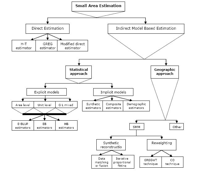
Figure 1

Download asset Open asset

A summary of different techniques for small area estimation (*after*<x> </x>Rahman, 2008a).

Figure 2

Download asset Open asset

A comparison of absolute distance and Chi-squared distance measures.

Figure 3

Download asset Open asset

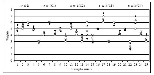
Plots of sampling design weights and new weights for specific cases.

Figure 4

Download asset Open asset

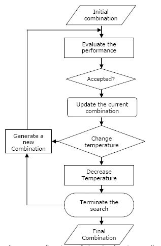
A flowchart of the simulated annealing algorithm (*after* Pham & Karaboga, 2000).

Figure 5

Download asset Open asset

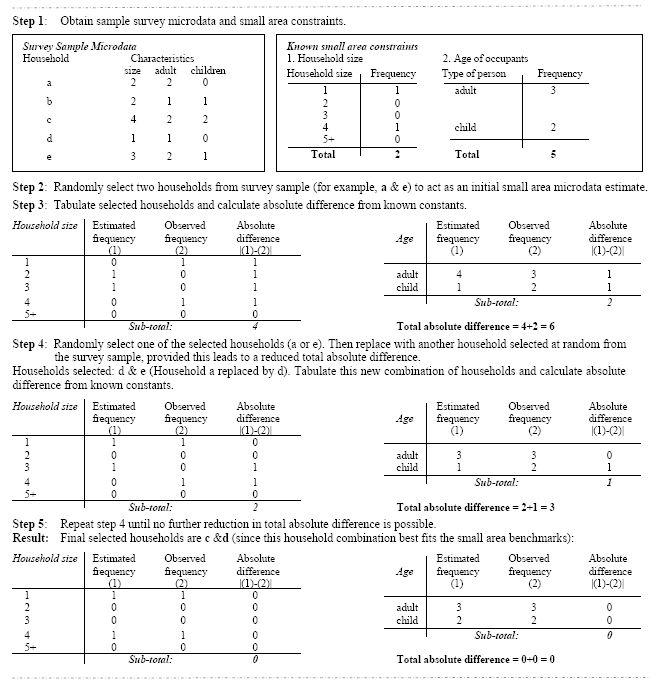
A simplified combinatorial optimisation process (*after* Huang & Williamson, 2001).

Figure 6

Download asset Open asset

A diagram of a prospective tool for generating spatial microdata.

Figure a-1

Download asset Open asset

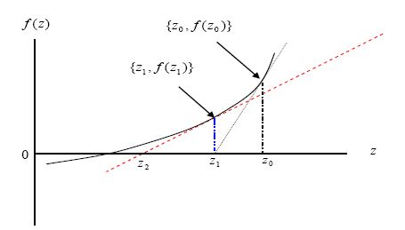
Graphical view of the Newton-Raphson iteration process.

Tables

Table 1

A brief summary of different methods for direct and indirect statistical model based small area estimation.

Small Area Estimation			Formula/model¹	Methods/Comments	Advantages	Disadvantages	Applications
Direct	Horvitz-Thompson estimator		${\hat{Y}}_{i} = \sum_{k \in s_{i}} d_{i k} y_{i k}$	Only based on real sample units.	Easy to calculate and unbiased for large samples.	It is unreliable and can not use auxiliary data.	Only if sample size is large enough.
	Generalised regression or GREG estimator		${\hat{Y}}_{i} = {X^{'}}_{i} \hat{β} + \sum_{k \in s_{i}} d_{i k} (y_{i k} - {x^{'}}_{i k} \hat{β})$	Based on real data and weighted least square (WLS) estimate of regression coefficient.	Can use auxiliary data at small area level, and approximately design and model unbiased.	It could be negative in some cases and not a consistent estimator due to high residuals.	When sample size is large and reliable auxiliary data are available at small area level.
	Modified direct estimator		${\hat{Y}}_{i} = {\hat{Y}}_{i} + (X_{i} - {\hat{X}}_{i})^{'} \hat{β}$	Based on real sample, auxiliary data and WLS estimate of regression.	Design unbiased and uses overall aggregated data for coefficient estimation.	Borrows strength from the overall data but can not increase effective sample.	When the overall sample size is large and reliable.
Indirect modelling	Implicit models	Synthetic estimator	${\hat{Y}}_{i} = \sum_{j} (X_{i j} / X_{j}) {\hat{Y}}_{j}$	Requires actual sample and auxiliary data for a large scale domain.	Straightforward formula and very easy and inexpensive to calculate.	All small areas are similar to large area assumption is not tenable & estimate is biased.	Used in various areas in government and social statistics.
		Composite estimator	${\hat{Y}}_{i} = ϕ_{i} {\hat{Y}}_{i [D]} + (1 - ϕ_{i}) {\hat{Y}}_{i [s]}$	Based on direct and synthetic estimators.	Have choices of balancing weight at small areas.	Biased estimator; depends on the chosen weight.	If direct and synthetic estimates are possible.
		Demographic estimator	${\hat{P}}_{i t} = \frac{1}{2} (\frac{b_{i t}}{{\hat{r}}_{i t}^{b}} + \frac{d_{i t}}{{\hat{r}}_{i t}^{d}})$	Rooted in data from census, and with time dependent variable.	Easy to estimate, and the underlying theory is simple and straightforward.	Only used for population estimates and affected by miscounts in census data.	Used to find birth and death rates and various population estimates.
	Explicit models²	Area level	${\hat{θ}}_{i} = {x^{'}}_{i} β + ε_{i} + e_{i}$	Based on a two stages model and known as the Fay-Herriot model.	Can use area specific auxiliary data and direct estimator.	Assumptions of normality with known variance may untenable at small sample.	Various areas in statistics fitting with assumptions of the model.
		Unit level	$y_{i j} = {x^{'}}_{i j} β + ε_{i} + e_{i j}$	Based on unit level auxiliary data and a nested error model.	Useful for continuous value variables, two stage and multivariate data.	Validating is quite complex and unreliable.	Used successfully in many areas of agricultural statistics.
		General linear mixed model	$y = X β + Z ε + e$	A general model, which encompasses all other small area models.	Can allow correlation between small areas, AR(1) and time series data.	Calculation and structure of matrix for area random effects are very complex.	In all areas of statistics where data are useful for the general model.

1

All usual notations are utilized (see Rahman, 2008a for details).
2

Methods such as empirical best linear unbiased predictor (E-BLUP), empirical Bayes (EB) and hierarchical Bayes (HB) are frequently used in explicit model based small area estimation. An excellent discussion of each of these complex methods is given in Rao (2003), and also in Rahman (2008a).

Table 2

Synthetic reconstruction versus the reweighting technique.

Synthetic reconstruction	Reweighting technique
• It is based on a sequential step by step process – where the characteristics of each sample unit are estimated by random sampling using a conditional probabilistic framework. • Ordering is essential in this process (each value should be generated in a fixed order). • Relatively more complex and time consuming. • The effects of inconsistency between constraining tables could be significant for this approach due to a mismatch in the table totals or subtotals.	• It is an iterative process – where a suitable fitting between actual data and the selected sample of microdata should be obtained by minimizing distance errors. • Ordering is not an issue. However convergence is achievable by repeating the process many times or by some simple adjustment. • The technique is complex from a theoretical point of view, it is comparatively less time consuming. • Reweighting techniques can allow the choice of constraining tables to match with researcher and/or user requirements.

Synthetic reconstruction

Reweighting technique

• It is based on a sequential step by step process – where the characteristics of each sample unit are estimated by random sampling using a conditional probabilistic framework.
• Ordering is essential in this process (each value should be generated in a fixed order).
• Relatively more complex and time consuming.
• The effects of inconsistency between constraining tables could be significant for this approach due to a mismatch in the table totals or subtotals.

• It is an iterative process – where a suitable fitting between actual data and the selected sample of microdata should be obtained by minimizing distance errors.
• Ordering is not an issue. However convergence is achievable by repeating the process many times or by some simple adjustment.
• The technique is complex from a theoretical point of view, it is comparatively less time consuming.
• Reweighting techniques can allow the choice of constraining tables to match with researcher and/or user requirements.

Table 3

New weights and its distance measures to sampling design weights.

d_k	w_k	w_k −d_k	$\overset{χ^{2}}{G_{k}}$
4	4.70844769	0.70844769	0.06273727
5	5.39271424	0.39271424	0.01542245
6	6.10925911	0.10925911	0.00099480
5	4.77151662	−0.22848338	0.00522047
3	3.09225105	0.09225105	0.00141838
4	4.41695372	0.41695372	0.02173130
6	5.97439907	−0.02560093	0.00005462
4	4.00419164	0.00419164	0.00000220
5	5.15375174	0.15375174	0.00236396
3	3.41348379	0.41348379	0.02849481
5	5.69627800	0.69627800	0.04848031
4	4.45424007	0.45424007	0.02579175
3	3.48091381	0.48091381	0.03854635
6	4.63754748	−1.36245252	0.15468974
4	3.57588131	−0.42411869	0.02248458
5	5.00000000	0	0
6	6.47125708	0.47125708	0.01850694
3	3.10505151	0.10505151	0.00183930
6	6.10925911	0.10925911	0.00099480
4	4.00419164	0.00419164	0.00000219
5	4.97866589	−0.02133411	0.00004551
3	2.31877374	−0.68122626	0.07734487
5	5.88555961	0.88555961	0.07842158
4	4.55702240	0.55702240	0.03878424
3	3.41348379	0.41348379	0.02849481
		TAD = 9.21152591	D = 0.67286721

Table 4

A comparison of the GREGWT and CO reweighting methodologies.

GREGWT	CO
• An iterative process. • Use the Newton-Raphson method of iteration. • Based on a distance function. • Attempt to minimize the distance function subject to the known benchmarks. • Use the Lagrange multipliers as minimisation tools for minimising the distance function. • Weights are in fractions. • Boundary condition is applied to new weights for achieving a solution. • The benchmark constraints at small area levels are fixed for the algorithms. • Typically focus on simulating microdata at small area levels and aggregation is possible at larger domains. • All estimates have their own standard errors obtained by a group jackknife approach. • In some cases convergence does not exist and this requires readjusting the boundary limits or a proxy indicator for this nonconvergence. • There is no standard index to check the statistical reliability of the estimates. • The iteration procedure can be unstable near a horizontal asymptote or at local extremum. • An iterative process.	• Use a stochastic approach of iteration MCMC. • Based on a combination of households. • Attempt to select an appropriate combination that best fits the known benchmarks. • Use different techniques as intelligent searching tools in optimizing combinations of households. • Weights are in integers (but could be fractions). • There is no boundary condition to new weights. • The algorithm is designed to optimize fit to a selected group of tables, which may or may not be the most appropriate ones. Hence there may be a choice of benchmark constraints. • Offers a flexibility and collective coherence of microdata, making it possible to perform mutually consistent analysis at any level of aggregation or sophistication. • No information about this in literature. May be possible in theory but nothing available in practice. • There are no convergence issues. However, the finally selected household combination may still fail to fit user-specified benchmark constraints. • There is no standard index to check the statistical reliability of the estimates. • The iteration algorithm may able to avoid deceiving at local extremum in the solutions.

GREGWT

• An iterative process.
• Use the Newton-Raphson method of iteration.
• Based on a distance function.
• Attempt to minimize the distance function subject to the known benchmarks.
• Use the Lagrange multipliers as minimisation tools for minimising the distance function.
• Weights are in fractions.
• Boundary condition is applied to new weights for achieving a solution.
• The benchmark constraints at small area levels are fixed for the algorithms.
• Typically focus on simulating microdata at small area levels and aggregation is possible at larger domains.
• All estimates have their own standard errors obtained by a group jackknife approach.
• In some cases convergence does not exist and this requires readjusting the boundary limits or a proxy indicator for this nonconvergence.
• There is no standard index to check the statistical reliability of the estimates.
• The iteration procedure can be unstable near a horizontal asymptote or at local extremum.
• An iterative process.

• Use a stochastic approach of iteration MCMC.
• Based on a combination of households.
• Attempt to select an appropriate combination that best fits the known benchmarks.
• Use different techniques as intelligent searching tools in optimizing combinations of households.
• Weights are in integers (but could be fractions).
• There is no boundary condition to new weights.
• The algorithm is designed to optimize fit to a selected group of tables, which may or may not be the most appropriate ones. Hence there may be a choice of benchmark constraints.
• Offers a flexibility and collective coherence of microdata, making it possible to perform mutually consistent analysis at any level of aggregation or sophistication.
• No information about this in literature. May be possible in theory but nothing available in practice.
• There are no convergence issues. However, the finally selected household combination may still fail to fit user-specified benchmark constraints.
• There is no standard index to check the statistical reliability of the estimates.
• The iteration algorithm may able to avoid deceiving at local extremum in the solutions.

Download links

A two-part list of links to download the article, or parts of the article, in various formats.

Downloads (link to download the article as PDF)

Article PDF

Download citations (links to download the citations from this article in formats compatible with various reference manager tools)

BibTeX
RIS

Open citations (links to open the citations from this article in various online reference manager services)

Mendeley

Figures

A summary of different techniques for small area estimation (after<x> </x>Rahman, 2008a).

A comparison of absolute distance and Chi-squared distance measures.

Plots of sampling design weights and new weights for specific cases.

A flowchart of the simulated annealing algorithm (after Pham & Karaboga, 2000).

A simplified combinatorial optimisation process (after Huang & Williamson, 2001).

A diagram of a prospective tool for generating spatial microdata.

Graphical view of the Newton-Raphson iteration process.

Tables

A brief summary of different methods for direct and indirect statistical model based small area estimation.

Synthetic reconstruction versus the reweighting technique.

New weights and its distance measures to sampling design weights.

A comparison of the GREGWT and CO reweighting methodologies.

Download links

Downloads (link to download the article as PDF)

Download citations (links to download the citations from this article in formats compatible with various reference manager tools)

Open citations (links to open the citations from this article in various online reference manager services)