Pushing it to the edge: Extending generalised regression as a spatial microsimulation method
- University of Canberra, Australia
Cite this article
as: R. Tanton, Y. Vidyattama; 2010; Pushing it to the edge: Extending generalised regression as a spatial microsimulation method; International Journal of Microsimulation; 3(2); 23-33.
doi: 10.34196/ijm.00036
- Article
- Figures and data
- Jump to
Figures
Figure 1
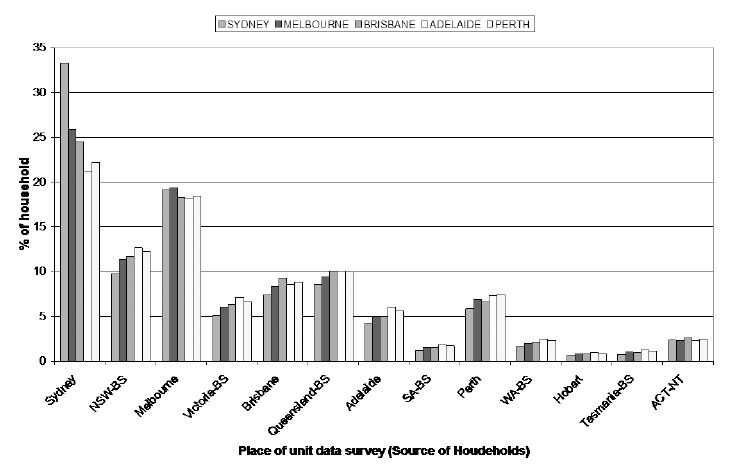
Source of households to populate SLAs in five capital cities.
Source: SpatialMSM/08c applied to SIH 2002/03 and 2003/04
Tables
Table 1
Benchmarks used in the procedures.
| Number | Benchmark |
|---|---|
| 1 | Age by sex by labour force status |
| 2 | Total number of households by dwelling type (Occupied private dwelling/Non private dwelling) |
| 3 | Tenure by weekly household rent |
| 4 | Tenure by household type |
| 5 | Dwelling structure by household family composition |
| 6 | Number of adults usually resident in household |
| 7 | Number of children usually resident in household |
| 8 | Monthly household mortgage by weekly household income |
| 9 | Persons in non-private dwelling |
| 10 | Tenure type by weekly household income |
-
Source: ABS Census of Population and Housing, 2006
Table 2
Number of SLAs dropped due to failed total absolute error.
| State/Territory | SLAs with failed TAE | Total SLAs | Percent of SLAs with failed TAE | Percent of population in SLAs with failed TAE |
|---|---|---|---|---|
| NSW | 2 | 200 | 1.0 | 0.4 |
| VIC | 4 | 210 | 1.9 | 0.0 |
| QLD | 43 | 479 | 9.0 | 0.8 |
| SA | 7 | 128 | 5.5 | 0.4 |
| WA | 17 | 156 | 10.9 | 0.9 |
| TAS | 1 | 44 | 2.3 | 0.1 |
| NT | 48 | 96 | 50.0 | 25.2 |
| ACT | 16 | 109 | 14.7 | 1.0 |
| Australia | 138 | 1422 | 9.7 | 0.7 |
-
Source: SpatialMSM/08c
Table 3
List of univariate benchmarks.
| Number | Benchmark table |
|---|---|
| 1 | Labour force status |
| 2 | Age |
| 3 | Sex |
| 4 | All household type |
| 5 | Tenure type |
| 6 | Weekly household rent |
| 7 | Household type |
| 8 | Dwelling structure |
| 9 | household family composition |
| 10 | Number of adults usually resident in household |
| 11 | Number of kids usually resident in household |
| 12 | Monthly household mortgage |
| 13 | Weekly household income |
| 14 | Persons in non-private dwelling |
Table 4
Summary of the impact of additional benchmarks.
| Model | SLAs with TAE < 1 | SLAs with TAE >= 1 | Measure of Accuracy |
|---|---|---|---|
| SPATIALMSM08c (11BM) | 1284 | 138 | 0.9307 |
| 11BM + non school Qualification (NSQ) BM | 1280 | 142 | 0.9268 |
| 11BM + Occupation (OCC) BM | 1262 | 160 | 0.9411 |
| 11BM + NSQ + OCC BM | 1257 | 165 | 0.9388 |
-
Source: SpatialMSM/08c applied to SIH 2002/03 and 2003/04
Table 5
Summary of the impact of using univariate benchmarks.
| Model | Accepted SLAs with TAE < 1 | SLAs with TAE >= 1 | SEI |
|---|---|---|---|
| SPATIALMSM/08c (11BM) | 1284 | 138 | 0.9307 |
| Univariate BM | 1329 | 93 | 0.8781 |
| Univariate BM and 1284 SLAs converged in SPATIALMSM/08c | 0.9100 |
-
Source: SpatialMSM/08c applied to SIH 2002/03 and 2003/04
Table 6
Effect of using households from each capital city to estimate areas in the capital city using spatial microsimulation.
| Source of data for estimation with SPATIALMSM/08c (11BM) | Number of sample used | Accepted SLAs with TAE < 1 | SLAs with TAE >= 1 | SEI |
|---|---|---|---|---|
| − Sydney for Sydney | 2831 | 63 | 1 | 0.9676 |
| − Australia for Sydney | 23,031 | 63 | 1 | 0.9618 |
| − Melbourne for Melbourne | 3129 | 78 | 1 | 0.9263 |
| − Australia for Melbourne | 23,551 | 79 | 0 | 0.9511 |
| − Brisbane for Brisbane | 1778 | 214 | 1 | 0.9263 |
| − Australia for Brisbane | 23,668 | 212 | 3 | 0.9224 |
| − Adelaide for Adelaide | 1824 | 55 | 0 | 0.9735 |
| − Australia for Adelaide | 23,603 | 55 | 0 | 0.9534 |
| − Perth for Perth | 1999 | 35 | 2 | 0.8478 |
| − Australia for Perth | 23,552 | 35 | 2 | 0.7856 |
-
Source: SpatialMSM/08c applied to SIH 2002/03 and 2003/04
Download links
A two-part list of links to download the article, or parts of the article, in various formats.