Alignment and matching in multi-purpose household microsimulations
- 284 Albert Road, Australia
Abstract
Household microsimulations are often required to align with deterministic projections from other sources. This paper suggests the use of random sampling within alignment pools to give one-pass event alignment. An iterative process is suggested for alignment of person types, but gives disturbingly high numbers of changes. Type alignment may be better done by manually adjusting assumptions to give approximate alignment.
Many forms of matching are needed in household microsimulations. The paper suggests two different immediate matching methods – probability-weighted, and best of n. Performance measures are derived for these methods, and for two existing batch methods – stochastic and order of decreasing difficulty. Probability-weighted matching gave slightly better results than best of n and stochastic, and order of decreasing difficulty gave poor results. The suggested matching methods may be useful in a wide range of applications.
1. Introduction
Although dynamic household microsimulation models are often used to help policy decisions by national governments, projections at regional and sub-regional levels are potentially useful to state and local governments. Models at fine geographic scales can also be commercially useful, for example to the developers of retirement care facilities. Such models require detailed assumptions about location choices, and large numbers of persons being modelled. Some models, such as SVERIGE (Holm, Holme, Makilla, Maffsson-Kauppi & Mortvik, 2004), ILUTE (Miller 2008) and Moses (Wu, Birkin & Rees, 2009) have attempted to meet these challenges.
Although the model described by Orcutt, Greenberger, Korbel and Rivlin (1961) had monthly projection cycles, nearly all subsequent models have had yearly cycles. The APPSIM model is designed to allow monthly cycles (Percival 2007). Short cycles help overcome the simulation errors identified by Galler (1997), and allow a wider range of uses. For example, monthly cycles are needed to simulate the aggressive development of diseases such as cancer.
The last decade has seen a more critical approach to the performance of household microsimulation models. Bouffard, Easther, Johnson, Morrison and Vink (2001) noted the poor results from the widely used stable marriage algorithm, and Leblanc, Morrison and Redway (2009) found poor results from stochastic and order of decreasing difficulty matching. These are three forms of batch matching, where persons to be matched are selected during a cycle, and paired off at the end of the cycle. Some models use immediate matching, where a person is selected to be matched, and a match found immediately.
This paper suggests one alignment and two matching methods, which may help meet present and new needs for microsimulation models. The suggested methods are unlikely to help reduce the wide disparities between run times of current national models, as these may reflect programming and data storage issues, as well as excessive use of alignment.
2. General comments on alignment
Orcutt, Greenberger, Korbel and Rivlin (1961) described an alignment process where event probabilities during each monthly simulation cycle were adjusted to try to eliminate any accumulated discrepancies with external control totals. Morrison (2006) described the evolution of alignment, identifying two needs – consistency with beliefs about the future, and elimination of stochastic variation.
Governments may have national population projections that underpin planning in many areas. Household microsimulations for policy purposes need to have assumptions consistent with those in the national projections, and give comparable results to them. As Morrison notes, even when considerable care and expertise are used in estimating behavioural equations from past data, very rarely do the microsimulations match expectations about the future. Harding (2007:12) asks whether aligning everything at a very disaggregated level may reduce the predictive usefulness of the dynamic model, by imposing upon the micro results predetermined macro outcomes.
Morrison (2006:16) comments that clients almost invariably prefer point estimates, and do not usually value information about likely distributions of results. This is not universal. For example, regulatory authorities for insurers now want information on the range of possible results, including unlikely but costly disasters. Many investors want to understand the risks and potential returns from each investment, as well as the risk reductions from diversification. The use of alignment to eliminate stochastic variation may thus be concealing valuable information. Note however that stochastic variation during a projection may only be a minor source of overall uncertainty. Uncertainties inherent in the estimation of model coefficients, and changes over time in individual behavior, government policy and economic conditions may be much greater sources of uncertainty.
Morrison (2008: 20) notes that DYNACAN had been misinterpreting mortality coefficients inherited from CORSIM, and that alignment had masked the misinterpretation. This appears to be one of the risks of using alignment, where a major underlying error may lead to a variety of distortions. A wide range of problems can cause microsimulation results to differ from national projections. For example, low births may result from low partnering rates or wrong age assumptions about immigrants. Wherever possible, it seems better to correct such problems early, rather than during alignment.
Three types of alignment may be needed
event alignment, for numbers of events such as births and deaths
state alignment, for numbers in particular states (for example, married persons in a particular age group and area)
monetary alignment, for totals such as wages.
Sometimes it may be possible to use event alignment to achieve the desired numbers of persons in particular states. In Australia, however, no national projections exist of partnership formations or dissolutions, forcing the use of state alignment to national projections of partner numbers. Another problem is that a single household exit can change household types in both the source and destination household, requiring an iterative state alignment process. A two-tier monetary alignment process is described by Dekkers et al. (2009: 4–5).
3. Event alignment
This section describes two existing methods of event alignment, and suggests a third. The performance of the three methods is tested by looking at mean ages at death.
In 1995 Baekgaard suggested a “sampling by sorting” alignment method where events are randomly simulated, and any departure from the alignment total corrected by reversing the outcomes of those events where the generated random number is closest to the probability of occurrence (see Baekgaard 2002: 12). This is the first of the methods tested here.
In 2001 Johnson proposed “alignment by sorting”, a method also involving reversing some of the simulated events. For each prospective event i, a value vi is calculated, where
vi = f(ri) − f(pi)
f(x) has the form -In( (1-x)/x )
pi is the prospective event’s probability
ri is a random number drawn from a (0,1) distribution.
The prospective events with the lowest vi magnitudes are then reversed to match the alignment total. In 2006, this was DYNACAN’s primary alignment method (Morrison 2006 p6). This is the second of the methods tested here. It is similar to sampling by sorting, except that both the probability and the random number are transformed before selecting events for reversal.
If random selection is being used to select persons for event testing, then alignment can be included in the process
randomly select an individual to be tested for the event
compare a random number with the event probability for that individual, and decide if the event occurs
repeat until the desired event total is reached.
This is the third of the methods tested here, and is called “alignment by random selection”.
One simple test of an alignment method is to measure the mean age of persons experiencing an event, without and with alignment. Any large age difference is an indication that the alignment method is flawed. For example, the first row of Table 1 shows that the mean age of death, when 20 different simulations were made of deaths in a year from 20,000 persons without alignment, was 77.57 years. The ages of these persons were representative of Australians in 2001. Using sampling by sorting, the observed mean age at death was 86.88 years when the alignment total was 63 per cent of the unaligned mean number of deaths, and 69.16 years when the alignment total was 127 per cent of the unaligned mean number of deaths.
Mean ages at death.
| Alignment method | Not aligned | Aligned to 63% of mean | Aligned to 100% of mean | Aligned to 127% of mean |
|---|---|---|---|---|
| Sampling by sorting | 77.57 | 86.88 | 76.93 | 69.16 |
| Alignment by sorting | 77.57 | 77.82 | 77.53 | 77.21 |
| Random selection | 77.24 | 77.22 | 77.27 | 77.06 |
The second row of Table 1 shows that much better results were obtained with alignment by sorting, again making 20 different simulations of deaths in a year from 20,000 persons without and with alignment. The observed mean age was 77.82 years when the alignment total was 63 per cent of the unaligned mean number, and 77.21 years when the alignment total was 127 per cent of the unaligned mean number. Both are close to the unaligned mean age at death of 77.57 years.
The third row of Table 1 shows that even better results were obtained with alignment by random selection. For this method, 3 simulations were made of the deaths in a year from 175,044 persons, based on a 1 per cent sample of Australians in 2001. The observed mean age was 77.22 years when the alignment total was 63 per cent of the unaligned mean number, and 77.06 years when the alignment total was 127 per cent of the unaligned mean number. Both are close to the unaligned mean of 77.24 years.
As shown in Table 1, sampling by sorting only works reasonably for alignment totals close to expected means. Because alignment is done by reversing the outcomes of those events where the generated random number is closest to the probability of occurrence, most reversals occur at the young ages. An alignment total below the mean thus leaves most of the old deaths unchanged, and gets rid of many of the younger deaths, giving a high average age on death.
The probability transformation used in alignment by sorting means that reversals occur where the difference between the log of the probability and the log of the random number is small. Reversals should thus be shared fairly evenly between young and old deaths, leaving the average age at death reasonably stable. Alignment by random selection does not involve any event reversals, and should not alter average ages. Trials showed no correlation between the between the ages at death of consecutively simulated deaths, or between their file positions.
4. State alignment of person numbers, ages and types
4.1 Test data and alignment pools
The Australian Bureau of Statistics estimated the resident population of Australia at 30 June 2001 as 19.482m. Their 1 per cent sample of the August 2001 census returns gave unit records for 188,013 persons, living in 75,451 households. As the sample was based on location at census night, rather than usual location, there were some incomplete households, with missing partners or children without adults. Omitting clearly incomplete families left 175,044 persons.
For the sample of 1,75,044 Australians, alignment was carried out separately for 8 areas (each state and the Australian Capital Territory). Births in each cycle were aligned for 4 age groups (15–24, 24–34, 35–44, 45–54), and deaths, emigration and immigration were aligned over 9 age groups (0–14, 15–24, …75–84,85+). Numbers of persons, and births, deaths, emigrants and immigrants were aligned against national projections (Australian Bureau of Statistics, 2003a). As the necessary details by age group and area were not published, they were obtained from a deterministic projection program closely replicating the national population projections.
4.2 Multi-stage alignment of numbers, ages and types of persons
Where alignment by number, age and type was needed for each area, it was found easier to do this in a three-stage process
alignment of the total numbers of persons in each age group, for Australia as a whole (9 alignment pools)
alignment of the total numbers of persons in each age group, for each area (72 pools)
alignment of the total numbers of persons of each type in each age group, for each area (576 pools).
Table 2 shows numbers of household changes, without and with alignment. Most of the entries in Table 2 relate to exits, where an “exit” is a departure from a household of a person, possibly followed by one or more of the other household members. By contrast, a “move” is where the whole household moves to another dwelling. A “normal” exit is one simulated using the assumed probabilities of exit, rather than an exit artificially created for alignment purposes. Ideally, few extra exits should be needed for alignment.
Numbers of household changes without and with alignment.
| Year | Normal exits (unaligned) | Normal exits (aligned) | Immigrants to align | State exits to align | Type exits to align |
|---|---|---|---|---|---|
| 0 | 0 | 0 | 892 | 1327 | 12,949 |
| 1 | 7588 | 7546 | 346 | 1134 | 9649 |
| 2 | 7766 | 7905 | 530 | 1178 | 9002 |
| 3 | 7792 | 7970 | 484 | 860 | 8945 |
| 4 | 8014 | 8213 | 403 | 1009 | 9137 |
| 5 | 8190 | 8505 | 563 | 1082 | 9764 |
| Average | 7870 | 8028 | 465 | 1053 | 9299 |
Normal exits are about 5 per cent of the initial sample population of 1,75,044 persons. The numbers of normal exits grow broadly in line with population increases, and are only slightly higher when event alignment is being used.
Table 2 shows large numbers of alignments at “year 0”, ie at the start of the projection. These alignments are needed to correct the under reporting inherent in the 1 per cent census sample used as the projection starting point. The Australian Bureau of Statistics does detailed post- census surveys to estimate the extent of census under-reporting, and uses these to publish “estimated resident populations”, the starting points for their population projections.
Three types of alignment were used at the start of the projection
alignment of the total numbers of persons in each of 9 age groups, done by simulating emigration by persons in over-represented ages, and immigration by those in under-represented ages (892 emigrants and 892 immigrants were needed)
alignment of the total numbers of persons in each age group in each of the 8 areas (done by 1,327 exits of individuals between areas)
alignment of the total numbers of persons of each of 8 person types, for each age group in each area (done by 12,949 exits of individuals within areas).
When using alignment, the numbers of births, deaths, emigrants and immigrants in each age group were exactly constrained to the numbers of these events derived from Australian national population projections. In theory, the correct number of persons in each age group at the end of the year should have automatically resulted. In practice, it was not possible to fully replicate the event numbers in the national projections, and small numbers of emigrants and emigrants were simulated to correct over or under-represented age groups (generally about 400 of each).
Movements between areas were simulated without constraint, using independently derived assumptions. At the end of each projection period exits between areas were simulated so as to bring the numbers in each age group in each area into line with national projections. Movements of exit “leaders” were simulated from areas where their age group was in surplus, to areas were in deficit. As exit leaders were sometimes followed by family members of varying ages, an iterative process was needed to reach equilibrium. Given the independent assumptions about movements between areas, it was pleasing that only about 1,000 simulated exits a year were needed to align area numbers. Given more knowledge of the movement assumptions underlying the national projections, fewer alignment exits might have been needed.
Numbers of partnership formations and breakups were not available from national projections. Alignments of persons of each type were done against the percentages of persons of each type and age group at the end of each year, which were available from Australian 25-year projections (Australian Bureau of Statistics 2004). Alignment was done in the following sequence
persons in non-private dwellings
lone parents
partners
children
related persons in family households
unrelated persons in family households
group households lone persons.
For example, if the number of partners in an area and age group was less than the alignment total, persons of the area and age group, not in non private dwellings, and not lone parents or partners, were randomly selected, and partners found for them by “best of n” matching. If the numbers of partners were too high, partners of the area and age group were selected, and their departure from partnership simulated. Restrictions were placed on the simulations used to align partner numbers, to avoid altering the numbers of lone parents. Some exits involved multiple persons, and could alter previously aligned totals in other age groups. An iterative process was used to reach equilibrium.
4.3 Average numbers of exits needed to correct misalignments
Table 3 shows the average numbers of exits needed to correct an area misalignment. A “misalignment” is a difference between an actual and a target number of persons in any pool, whether positive or negative.
Average number of exits per area misalignment.
| Year | Number of misalignments | Exits to correct Misalignments | Exits per misalignment |
|---|---|---|---|
| 0 | 2362 | 1327 | 0.56 |
| 1 | 1884 | 1134 | 0.60 |
| 2 | 2046 | 1178 | 0.58 |
| 3 | 1520 | 860 | 0.57 |
| 4 | 1770 | 1009 | 0.57 |
| 5 | 1822 | 1082 | 0.59 |
| Average 1–5 | 1808 | 1053 | 0.58 |
The total numbers of persons in the wrong areas were low, averaging about 1 per cent of the population during the first five projection years. On average, about 0.58 exits were needed to correct an area misalignment. This low number is because most of the simulated exits were of persons without followers, and each of these exits corrected a misalignment in the source area and the new area. By contrast, Table 4 shows that about 3 per cent of the population had the wrong household type in the first five years, and about 1.75 exits were needed to correct a type misalignment. No attempt was made to direct persons from one type in excess to another type in deficit, so that something over 1 exit per misalignment was expected (after allowing for the effects of followers).
In part, these high numbers of type misalignments were due to the use of 576 separate alignment pools (8 states, 9 ages and 8 types). The average number of normal exits in the first 5 years was about 8,000, which was about 14 per pool. Each exit is both a departure from a pool and an entry into another, so that on average each pool had about 28 exit changes a year. The net movement of persons in or out of the pool may be distributed about N(0,5.3), and the average number of misalignments may be about 4.2. This suggests that about 2,400 misalignments a year might occur if there were 576 equal alignment pools. Table 4 shows an average of 5,314 misalignments a year, and this higher number may reflect the considerable disparity in the numbers of expected exits from each of the alignment pools. The more alignment pools, the larger the numbers of likely type misalignments.
Average number of exits per type misalignment.
| Year | Number of misalignments | Exits to correct misalignments | Exits per misalignment |
|---|---|---|---|
| 0 | 11,194 | 12,949 | 1.16 |
| 1 | 5278 | 9649 | 1.83 |
| 2 | 5238 | 9002 | 1.72 |
| 3 | 4950 | 8945 | 1.81 |
| 4 | 5314 | 9137 | 1.72 |
| 5 | 5788 | 9764 | 1.69 |
| Average 1–5 | 5314 | 9299 | 1.75 |
5. Matching
5.1 Past and current matching methods
Many different types of matches may be needed in closed household microsimulations. For example, males and females may have to be matched to form partnerships, individuals matched to form groups, and households matched to dwellings.
Orcutt, Greenberger, Korbel and Rivlin (1961: 75–76) selected individuals to be married, and then used functions describing the relations between persons marrying to randomly select the characteristics of the partner. Individuals to be married were held in temporary storage until a person with the selected characteristics was identified during the pass through the household file. Orcutt, Caldwell and Wertheimer (1976: 34–35) selected males and females to be married during a year, then ranked them based on race, age, education and region. After the rank orderings of males and females were merged, the excess male or females who happened to fit least well were returned to the single population.
These two early processes have many of the features of matching processes used subsequently. In the model described in 1961, a marriage partner was found almost immediately for a person selected to be married. In the model described in 1976, males and females to be married were selected during the year, then merged in a batch process at the end of the year, with the poorest fits being rejected. Table 5 shows that immediate and batch matching methods have been used in recent models, with considerable diversity in their detail.
Matching methods used in some recent national models.
| Model name | Version | Immediate or batch | Matching method |
|---|---|---|---|
| APPSIM | 2009? | Immediate | Statistical selection from eligible partners |
| CBOLT | 2002? | Batch | Normalised match probabilities |
| DYNACAN | 2002? | Batch | Stochastic |
| DYNASIM3 | 2002? | Batch | Random within race, age & education |
| INAHSIM | 1986 | Batch | Merge by age order |
| MIDAS-BE | 2008 | Batch | Order of decreasing difficulty |
| Pensim2 | 2004 | Batch | Order of decreasing difficulty |
| SESIM | 1997 | Immediate | First male 3 years older in region |
| SMILE | 2005? | Batch | Order of decreasing difficulty |
| SVERIGE | 2002 | Batch | Replication of patterns of recent pairs |
-
Sources
APPSIM – Bacon and Pennec (2007: 19)
CBOLT – Perese (2002: 17)
DYNACAN – Leblanc, Morrison and Redway (2009: 6,11–12)
DYNASIM3 – Favreault and Smith (2004: 9)
INAHSIM – Inagaki (2009)
MIDAS – Dekkers et al. (2009: 33)
Pensim2 – Emmerson, Reed and Shephard (2004: 30)
SESIM – Petterson (2009)
SMILE – O’Donoghue, Lennon and Hynes (2009: 24)
SVERIGE – Holm, Holme, Makilla, Maffsson-Kauppi and Mortvik (2004: 20–23)
Bouffard, Easther, Johnson, Morrison and Vink (2001: 6) noted that the CORSIM, DYNACAN, POLSIM and SVIERGE models all used something similar to CORSIM’s stable marriage algorithm to form specific couples from pools of prospective marriage partners. In spite of its theoretical elegance, this was found to produce too many close partnerships, and too many distant ones.
Stochastic matching, proposed by Easther and Vink in 2000, calculates the relative probability of each potential pairing from two equal pools of males and females, and randomly selects a pairing on a probability-weighted basis. This proceeds sequentially until pairing is complete. This process was implemented in CORSIM and DYNACAN. Leblanc, Morrison and Redway (2009) tested stochastic matching, tournament selection and order of decreasing difficulty matching, and concluded that none gave good results, but stochastic matching was the best of the available methods. All the methods tested were batch methods.
Perese (2002: 17) proposed a sequential matching process for male and female pools, where the probabilities of marriage to a male are calculated for each remaining female, and normalized so that the highest probability is 1. For each female in turn, a random number is drawn, and a match made if the number is less than the calculated probability. As a result of the normalization, a match is always found. This process was implemented in CBOLT, apparently on a batch basis. INAHSIM selects equal numbers of males and females to be married, sorts both by age, them merges (Inagaki, 2009). SESIM randomly selects females in a region to be married, and creates a pool of all eligible males in the region. For each selected female in turn, a male 3 years older is selected. If no such male can be found, age differences of 2 to 4 years are considered (Petterson, 2009).
Leblanc, Morrison and Redway (2009) tested a modified version of a batch matching procedure by order of decreasing difficulty (ODD) proposed by Redway. Good matches are first made for those hardest to pair off, with pairing proceeding in order of decreasing difficulty. Although this algorithm did extremely well in terms of not creating marriages with extreme age differences, it also generated far too many marriages in which the husband is a single year of age greater than his wife. The authors suggested that the poor quality of the compatibility measure used prevented any true testing of matching procedures. Matching by order of decreasing difficulty is being used by PENSIM2, and by LIAM-based models such as SMILE (O’Donoghue, Lennon & Hynes, 2009) and MIDAS (Dekkers et al., 2009).
5.2 Suggested matching methods
This paper suggests the use of immediate probability-weighted matching. As soon as a male or female is simulated to marry, all the potential marriage partners for that person are identified. One of these potential partners is then randomly selected, with a procedure where a partner’s probability of selection is proportional to their probability of marriage to the person. Although this procedure appears similar to stochastic matching, there are important differences. Probabilities have to be those for marriage to randomly selected single persons, rather than to persons already selected to marry. The numbers of potential matches are much higher, so that calculation times can be much longer than for stochastic matching. As batches are not used, there is no problem with the last matches being unlikely.
The calculation times needed for immediate probability-weighted matching can be greatly reduced if selections are made from a small number of randomly sampled single persons, rather than from all single persons. Performance tests with sample sizes of 10, 20, 30, 50, 100 and 200 suggest that sample sizes of about 30 may be sufficient, at least for the Australian test data used (see Table 7). Calculation times should be directly proportional to the sample size, and to the total number of persons.
The paper also suggests the use of immediate “best of n” matching, where a number of potential partners are randomly selected from single persons, and the potential partner with the highest probability of marriage chosen. Trials show that the number of randomly selected potential partners needs to vary with the age of the person seeking a partner. For the Australian test data, the numbers needed were 6 at ages 18–19, 4 at ages 35–49, and 5 at all other ages. These low numbers make “best of n” matching a fast method. Calculation times will be proportional to the average value of n, and to the total number of persons.
5.3 Test data from persons married in Australia in 2002
Test data were derived from data on the ages of persons in 1,05,435 new marriages in 2002 (Australian Bureau of Statistics, 2003b). The published data show the cross-classified ages of brides and grooms in single-year age groups up to 54, then 55–59, 60–64, and 65 and over. In addition, the ages of males marrying are shown in single years up to age 74, then 75 and over, as are the ages of females marrying. The data showed very few persons marrying below age 18, and these persons were omitted from analysis, leaving 1,05,372 marriages. To fill the data gaps over age 54, it was assumed that, for each age of a male at marriage, the ages of brides were normally distributed. Normal distributions for each male age were obtained by minimising the sum of the squares of differences of the actual and fitted numbers for each single age or age-group. While this Australian data only contains ages, it is sufficiently detailed to test fitting methods, and to identify matching methods unlikely to work with more complex data. Its simplicity made it possible to write fast algorithms to exhaustively test different matching methods. The mean age differences in Figure 1, and their standard deviations, were obtained from the actual one-year data were available, and from the fitted normal curves where one-year data were not available. The mean age differences show that very young males tend to marry females a little older than themselves. After age 23 males become progressively older than their brides, with the estimated age difference being 6.8 years for males aged 54. The fitted standard deviation of female ages for males aged 18 is 3.9 years, dropping to 2.5 years at age 19, and then climbing to 7.6 years at age 54. The low numbers of persons marrying after age 54, and the unavailability of single-year data, create very wide confidence limits for the estimates for males over 54. The mean age difference and its standard deviation may in fact continue to increase with male ages well past 54.
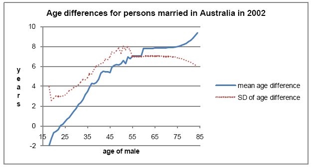
Age differences of persons married in Australia in 2002.
5.4 Performance measures and graphs for different matching methods
A variety of criteria have been used to test the validity of matching methods. If these criteria are too weak, then quite poor matching methods may be accepted as useful. As Figure 1 shows, age differences and age standard deviations for persons marrying are strongly dependent on the age of the male, and comparisons of overall age differences may fail to detect major problems at particular ages. Bouffard et al. (2001) used graphs of the percentages of couples with each age difference, as well as percentile graphs of compatibility levels. These graphs allow visual comparisons between the pairing results and population values. The authors noted (p. 4)
“…the synthetic marriages should resemble actual new marriages in both their central tendencies and their dispersion”
Graphs of means and standard deviations of age differences at marriage help assess the extent to which the synthetic marriages resemble actual new marriages. Graphs of the ratios of simulated to actual marriages for each probability percentile can show problems at the extremes, even where overall test statistics are reasonable.
Tables 6 and 7 use three different measures of goodness of fit
sum of squares of the differences between actual and simulated marriages for each age combination
chi square test statistics, calculated for each age combination for which at least five marriages are observed in the data
the standard deviation of the ratio of simulated to actual marriages for each probability percentile.
Performance measures for models fitted to Australian data.
| Probability model | Fitting method | Degrees freedom | Sum of squares | Chi square |
|---|---|---|---|---|
| Quadratic | Least squares | 1,309 | 672,472 | 4,880 |
| Gamma | Least squares | 1,242 | 1,576,369 | 8,323 |
| Quartic | Least squares | 1,175 | 727,746 | 4,397 |
| Piecewise quadratic | Least squares | 1,237 | 122,323 | 1,233 |
| Piecewise quadratic | Logistic | 1,237 | 214,934 | 1,468 |
Test results for different matching methods.
| Immediate/ Batch | Matching Method | Sample size | Sum of squares | Chi Square | Percentile SD |
|---|---|---|---|---|---|
| Immediate | Probability weighted | 10 | 1,026,008 | 5,476 | |
| Immediate | Probability weighted | 20 | 497,016 | 3,457 | |
| Immediate | Probability weighted | 30 | 364,242 | 3,049 | 0.068 |
| Immediate | Probability weighted | 50 | 308,535 | 2,816 | |
| Immediate | Probability weighted | 100 | 279,732 | 2,709 | |
| Immediate | Probability weighted | 200 | 259,819 | 2,700 | |
| Immediate | Best of n | 484,912 | 3,879 | 0.090 | |
| Batch | Stochastic | 105,372 | 409,197 | 5,636 | 0.078 |
| Batch | Order of decreasing difficulty | 105,372 | 185,184,957 | 621,141 | 1.485 |
| Batch | ODD/probability weighted | 105,372 | 2,214,049 | 12,395 |
Table 6 shows sum of squares and chi square performance measures obtained when fitting different relative probability models to the Australian test data described in 5.3. The lower the measures, the better the fit.
The first line in Table 6 was obtained by fitting relative probabilities of marriage, where the relative probability of a male age × marrying a female age y was defined as exp(score) / (1 + exp(score)), where
score = a + b(x − y) + c(x − y)2
x is the age of the male
y is the age of the female
and a, b and c are regression coefficients fitted for each separate male age.
As the fitting procedure provided no guidance as to the value of the regression constant a, it was held at -3 throughout. Regression coefficients b and c were fitted for each age of male by minimizing the sums of squares of the differences between the numbers of marriages with each combination of male and female ages. Fitting was done within a spreadsheet, using Excel’s Solver, fitting each year of age for males separately. Poor fits were obtained with the quadratic function, and also with gamma and quartic functions. A much better fit was obtained with piecewise quadratic functions, where one quadratic was fitted for all females below or equal to the male age, and a separate quadratic function fitted for all females above the male age. Only one quadratic was needed for each age from 60 on.
Chi square test statistics were calculated as
χ2 = ∑∑ (Oij − Eij)2/Oij
where Eij is the number of females age j expected to marry males of age i, as estimated from the fitted coefficients and equations and Oij is the number of females age j who did marry males of age i in 2002.
The chi square statistic was calculated by summing across all cells with at least 5 observed marriages. Observed marriages were used in the denominator, as this gave more stability when comparing different fits. The mean of a chi square distribution with k degrees of freedom is k, so that the piecewise quadratics gave a chi square statistic close to its expected value.
The last line of Table 5.2 was obtained by using logistic regression as described below, with 10 dummy records of non-marrying couples for each of the 105,372 records of couples marrying.
5.5 Fitting probabilities of marriage using logistic regression
CORSIM and DYNACAN used compatibility measures derived from logistic regression applied to census data. Variables used included age difference and its square, difference in years of education, number of children, race, labour force participation, earnings difference and some interaction effects (Bouffard et al., 2001, p. 5). The compatibility index was estimated using logistic regression on a potential pairs data file of recent marriages. The potential pairs may have included each possible pairing of the persons recently married, as well as the pairs which did marry (Perese, 2002: 9).
Logistic regression is widely used to estimate probabilities of events occurring, and the data needs to have some cases where the event occurs, and others where it does not. The addition of potential pairs is thus a device to make the regression feasible, and there is no need to add any particular number of potential pairs. Logistic regression fits probability models of the form
Score = β0 + ∑βixi
probability = exp (score) / (1+exp(score))
where βi are the fitted parameters, and xi the explanatory variables.
If the potential partner with the highest probability is to be selected, then comparisons can be made between regression scores, and the value of the constant β0 is immaterial. But if partners are to be selected on a probability-weighted basis, as in stochastic matching, then the value of β0 will matter. The number of potential pairs added for the regression analysis will thus have some effect on the results of stochastic matching.
For male ages 18 to 36, the logistic regressions gave positive quadratic coefficients for females older than the males. To avoid unrealistically high probabilities of marriage to much older females, it was initially assumed that probabilities of marriage to females more than 20 years older than males were zero. This expedient caused program errors during stochastic batch matching, and had to be abandoned. Instead, the quadratic component for males aged 18 to 36 was assumed to remain constant for females aged 12 or more years older.
Absolute probabilities of marriage are needed for immediate probability-weighted matching, and for batch stochastic matching. They were obtained by using Solver to find regression constants for each male age giving probabilities of marriage to females of each age summing to unity. The validity of this process is uncertain.
5.6 Test results for different matching methods
Table 7 shows performance measures for immediate probability-weighted matching, using sample sizes between 10 and 200. It also shows measures for immediate best of n matching, and for three different batch methods. As in Table 6, the lower the measure, the better the fit. Table 7 shows that the different goodness of fit measures give broadly similar results. Probability-weighted matching with samples of at least 30 gives slightly better results than best of n and stochastic, and order of decreasing difficulty gives very poor results.
5.7 Performance graphs for matching methods
From Figure 2, the average simulated age difference is quite close to those observed in Australian data, but with increasing random variations at older ages due to the small numbers of marriages. Apart from age 18, the simulated standard deviations are also quite close to observed values. For most practical purposes, the simulated marriages could be considered to be close enough to real marriage age distributions.

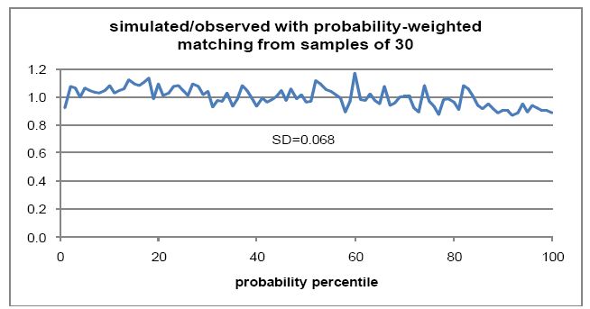
Age differences of persons with probability-weighted matching.
Figure 3 shows the numbers of fitted marriages, divided by the numbers of observed marriages, for each probability percentile. These percentiles were derived by taking each male/female age combination, calculating the relative probability of marriage, and sorting by probability. Numbers of observed marriages were then added, with each age combination being assigned to the probability percentile applying to its last member. This process resulted in probability percentiles averaging 1 per cent of marriages, but with some variations around this size. The simulated to observed ratios in Figure 3 have an average of 1.0, and a standard deviation of 0.068. This standard deviation is higher than the 0.031 expected from random variations in a sample size of 1,054. There appears to be a slight under-representation of high-probability marriages.

Percentile ratios for probability-weighted matching.
Graphs of cumulative probability distributions were used by Leblanc, Morrison and Redway (2009) to show relatively poor fits. When fits are reasonable, graphs of the fit within each probability percentile may be more useful. Probability percentiles remain useful l even with many explanatory variables.
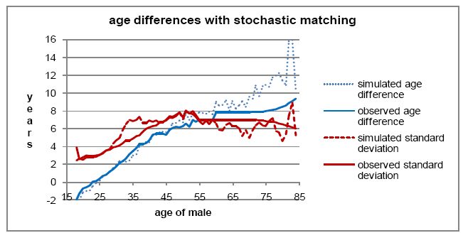
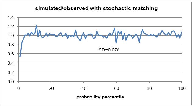
Figure 4 shows that average simulated age differences are higher than observed values from about age 50 on. Simulated standard deviations are a little high from about age 30 to 40. But for most practical purposes, the simulated marriages could be considered to be close enough to real marriage age distributions. Figure 5 shows a slight shortfall in simulated marriages for the first two probability percentiles. Overall, stochastic matching appears to be giving slightly inferior results to probability-weighted matching with samples of 30.

Age differences of persons with stochastic matching.

Percentile ratios for stochastic matching.
6. Conclusions
Household microsimulation models are being put to an increasing range of uses, some with challenging technical requirements. This paper suggests new alignment and matching techniques to help meet some of these challenges.
Event alignment can be readily done by random selection, without distortions. Initial misalignments are inevitable with census samples, and a systematic process for correcting them is needed. Alignment of person types during projections can produce large numbers of household changes, exaggerating household instability. The larger the numbers of alignment pools for person types, the more household changes will be needed for alignment. If approximate type alignment will suffice, this can be done by adjusting exit assumptions until the desired person type distributions are approximately obtained. In general, state alignment is much harder to do than event alignment, and if over-ambitious can cause severe distortions.
Household microsimulation models have used immediate or batch matching. This paper suggests two immediate matching methods – probability- weighted and “best of n”. Performance tests with Australian data show that both are likely to better reproduce partnership patterns than currently used batch matching methods. Probability-weighted matching can be greatly speeded by limiting the sample of potential partners to about 30, without much loss of fidelity. Immediate matching seems likely to give better matching and shorter run times, particularly when used with large populations, multiple regions and short time cycles.
This paper reflects the more rigorous evaluation of microsimulation techniques introduced by the dynacan team. The performance of different methods can be measured, and the best selected. Models that are slow, limited or unrealistic are unlikely to attract continuing funding.
References
-
1
Population projections Australia 2002–2101iii, catalog no 3222.0, Canberra, September, 3, + 186 pages, www.abs.gov.au.
-
2
Marriages and divorces Australia 2002, catalog no 3310.0, Canberra, November, 6, 92 pagesMarriages and divorces Australia 2002, catalog no 3310.0, Canberra, November, 6, 92 pages.
-
3
+ 138 pagesiii, Household and family projections Australia 2001 to 2026, catalog no 3236.0, Canberra, June, 18, + 138 pages, www.abs.gov.au.
-
4
APPSIM – modelling family formation and dissolution. Working Paper no 4v, APPSIM – modelling family formation and dissolution. Working Paper no 4, National Centre for Social and Economic Modelling, Canberra, November, + 29 pages.
-
5
Micro-macro linkage and the alignment of transition processes – some issues, techniques and examples. Technical Paper No 25v, Micro-macro linkage and the alignment of transition processes – some issues, techniques and examples. Technical Paper No 25, National Centre for Social and Economic Modelling, University of Canberra, June, + 29 pages.
-
6
Matchmaker, matchmaker, make me a matchJoint CORSIM and DYNACAN Project Document, September, 19 pages (also in Brazilian Electronic Journal of Economics, vol 4, no 2).
-
7
What are the consequences of the AWG-projections for the adequacy of social security pensions?. ENEPRI Research Report No 65 AIM WP4What are the consequences of the AWG-projections for the adequacy of social security pensions?. ENEPRI Research Report No 65 AIM WP4, January, 340 pages, www.enepri.org.
-
8
A stochastic marriage market for CORSIM. Strategic Forecasting Technical ReportA stochastic marriage market for CORSIM. Strategic Forecasting Technical Report, October, 8 pages.
-
9
An assessment of Pensim2. The Institute for Fiscal Studies. WP04/21An assessment of Pensim2. The Institute for Fiscal Studies. WP04/21, London, 51 pages.
-
10
A primer on the dynamic simulation of income model (DYNASIM3), The Urban Institute, Washington DC, February, 22 pagesA primer on the dynamic simulation of income model (DYNASIM3), The Urban Institute, Washington DC, February, 22 pages.
-
11
National Centre for Social & Economic Modellingv, Discrete time and continuous-time approaches to dynamic microsimulation reconsidered. Technical Paper No 13, National Centre for Social & Economic Modelling, Canberra, October, + 35.
-
12
Challenges and opportunities of dynamic microsimulation modellingplenary paper to the first general conference of the International Microsimulation Association, Vienna, August 21, 23 pages.
-
13
The SVERIGE spatial microsimulation model – content, validation, and example applicationSpatial Modelling Centre, Kiruna, Sweden, 74 pages, www.umu.se.
- 14
-
15
Nonlinear alignment by sorting. CORSIM Working PaperNonlinear alignment by sorting. CORSIM Working Paper, February.
-
16
A match made in silicon: Marriage matching algorithms for dynamic microsimulationpaper presented to the second general conference of the International Microsimulation Association, Ottawa, June 8–10, 27 pages.
-
17
v, Development of an operational integrated urban model system – volume I project final report, Urban Transport Research 7 Advancement Centre, University of Toronto, December, + 95 pagesv, Development of an operational integrated urban model system – volume I project final report, Urban Transport Research 7 Advancement Centre, University of Toronto, December, + 95 pages.
-
18
DYNACAN Team, 7th floor, Narono Building, 360 Laurier Avenue WestMake it so: event alignment in dynamic microsimulation, DYNACAN Team, 7th floor, Narono Building, 360 Laurier Avenue West, Ottawa, Ontario, May, 21 pages.
-
19
Validation of longitudinal microsimulation models. National Centre for Social and Economic Modelling, University of Canberra. Working Paper No 8Validation of longitudinal microsimulation models. National Centre for Social and Economic Modelling, University of Canberra. Working Paper No 8, March, 41 pages.
-
20
The life-cycle income analysis model (LIAM): A study of a flexible dynamic microsimulation modelling computing frameworkInternational Journal of Microsimulation 2:16–31.
-
21
vxiii, Microanalysis of socioeconomic systems - a simulation study, Harper & Brothers, New York, + 425vxiii, Microanalysis of socioeconomic systems - a simulation study, Harper & Brothers, New York, + 425.
-
22
xvi, Policy exploration through microanalytic simulation, The Urban Institute, Washington DC, + 370xvi, Policy exploration through microanalytic simulation, The Urban Institute, Washington DC, + 370.
-
23
National Centre for Social and Economic ModellingAPPSIM – software selection and data structures, National Centre for Social and Economic Modelling, Canberra, working paper no 3, April, 15 pages.
-
24
Technical Paper 2002-3Mate matching for microsimulation models, Technical Paper 2002-3, Long-term Modelling Group, Congressional Budget Office, Washington DC, 32 pages.
- 25
-
26
A hybrid spatial microsimulation model for decision support in demographic planning. paper presented to the second general conference of the International Microsimulation AssociationA hybrid spatial microsimulation model for decision support in demographic planning. paper presented to the second general conference of the International Microsimulation Association, Ottawa, June 8–10, 17 pages, http://www.microsimulation.org/IMA/Ottawa_2009.htm15/11/09.
Article and author information
Author details
Acknowledgements
I am very grateful for help received from Gijs Dekkers, Richard Easther, Seiichi Inagaki, Rick Morrison, Cathal O’Donoghue, Tomas Petterson and Howard Redway.
Publication history
- Version of Record published: December 31, 2010 (version 1)
Copyright
© 2010, Cumpston
This article is distributed under the terms of the Creative Commons Attribution License, which permits unrestricted use and redistribution provided that the original author and source are credited.