On the Italian ACE and its impact on enterprise performance: A PLS-path modeling analysis
- University of Cassino, Department of Economics, Italy
- ISTAT, Italy
Abstract
In 1998 Italy introduced a restricted version of an Allowance for Corporate Equity, called Dual Income Tax. Using data integrating Italy’s Institute for Statistics enterprise survey data and company accounts, we explore the effects of the Dual Income Tax on enterprise performance in 1998–2001. Firms benefiting from this allowance are simulated through the DIECOFIS corporate tax microsimulation model. The method to estimate enterprise performance is based on a structural equation model which allows us to compute a composite indicator given specific factors observed from enterprise activity. We find a positive impact of the Dual Income Tax on enterprise performance in that companies benefiting from this allowance outperformed non-eligible ones.
We thank two anonymous referees for their constructive comments on a previous version of this paper, participants at the Pre-ICM Convention on Mathematical Sciences (December 2008, Delhi) and at the Second Congress of the International Microsimulation Association (June 2009, Ottawa) where this paper was presented, and Paolo Roberti. The results discussed here rely on micro data from Italy’s Institute for Statistics (ISTAT) SCI and PMI surveys and company accounts data from the Italian Chamber of Commerce, both available at ISTAT within the DIECOFIS project funded by the Information Society Technologies Programme (IST-2000-31125) of the European Commission. ISTAT bears no responsibility for analysis or interpretation of the data. The usual disclaimer applies.
1. Introduction
Economic efficiency, usually identified with neutrality, is by far the most important consideration when designing a corporate tax system. Generally speaking, a tax on firms is efficient when it leaves the firm behaviour unchanged after taxation, that is when decisions undertaken by the firm are unaffected by the presence of the tax. The efficiency features of a corporate tax system can be studied regarding the investment decisions of the firm as well as its financing policy. The latter aspect has received great attention both in the theoretical and empirical literature.
As well known from the theory, in the absence of taxation and imperfections in the capital markets and information, firms are indifferent whether they finance their investments through debt or equity capital. This result changes when taxes are introduced. As the firm has three main financing sources, i.e. debt, retained earnings, and new shares issues, it can be demonstrated that the corporate tax system is neutral over the company financing decisions if the flow of before-tax profits remains unchanged after taxes for marginal investors, whether the return for investors takes the form of interest, dividends or capital gains. The corporate tax changes this picture as interest payments are usually deductible from the tax base while dividends are not; in this sense a corporate tax is not neutral over the company funding sources in that it favours debt over equity financing. The magnitude of these distortions then depends on the features of the corporate tax and personal tax regimes.
Specific systems can be proposed to address this issue. In 1991, the Institute for Fiscal Studies (1991) suggested introducing an allowance for corporate equity (ACE). The basic idea was to provide a deduction of a notional return on company equity from taxable profits so as to address the difference in the tax treatment of debt and equity. In recent years such systems have been in operation in some EU countries (for instance, besides Italy, Croatia, Austria and Belgium), though with differences in their practical application (Klemm, 2007). However, in recent years most of these countries have scrapped these systems, offering different motivations.
An ACE system has a number of attractive properties. The first obvious feature is that it meets neutrality between debt and equity financing if tax parameters are chosen correctly. The second feature is that as the tax is not levied on the marginal investment, this system is neutral to firm investment decisions. Another property is that the system offsets the distortion originated by the difference between depreciation for tax purposes and economic depreciation (Boadway & Bruce, 1984), as the advantage generated by tax depreciation is fully compensated by the reduction of (future) allowances. In this sense an ACE is again neutral over company investment decisions.
One negative feature of an ACE regime is that as the tax is only levied on extra profits it narrows the tax base and therefore the statutory rate must be greater compared to a standard system to collect the same tax revenue. In a tax competitive environment where governments tend to reduce capital taxation, an ACE regime might deter multinational companies from locating their investments within the country. This motivation probably lay at the heart of policy-makers’ decisions to dismantle the systems in countries where they were implemented.
In 1998 Italy introduced a restricted version of an ACE, called Dual Income Tax (DIT). This was part of a comprehensive reform that had the primary aim of a selective reduction in the burden of taxation so as to reduce the tax distortion between equity and debt financing. Under the DIT scheme a lower statutory rate is applied to the portion of profits representing the opportunity cost of new equity financing compared with other forms of capital investment. This system structurally reduced the corporate tax burden depending on the amount of the capital increase (new capital subscription and retained earnings) carried out by the company. It remained in place until 2004 when it was definitively abolished, although in July 2001, when a new government took office, some modifications to the original regime were adopted in order to rein in its effects. Several studies provide an assessment of the ACE systems, both for Italy and other countries (again see Klemm, 2007, for a review). In Italy these studies concentrate on the impact of the DIT system on the company tax rate and the neutrality features of this regime with respect to the pre-existing one as well as the subsequent system.
Given that the primary policy objective of the DIT allowance was to reduce the tax discrimination against equity financing and strengthen the financial structure of Italian companies, this regime might have had a positive impact on their performance. We expect three factors to work in this direction. First, the reduction in the cost of equity-funded investment capital has an impact on firms (usually small) with constraints on debt financing or in general on firms for which access to the credit market is more difficult. Secondly, as over-reliance on debt financing can be viewed as a potential threat to the financial stability of the corporate sector, the increase in firms’ capitalization improves the competitive position of companies benefiting from the allowance. Lastly, the reduction in the effective tax rate obviously increases firm profitability.
In this paper we study the impact of DIT on enterprise performance. Our empirical analysis is restricted to the period 1998–2001 when the system was in “full" operation and is based on a specific dataset combining ISTAT (Italy’s Institute for Statistics) survey data on firms and company accounts. Data do not include companies of the agricultural and financial sectors.
To this end we estimate a Structural Equation Model (herein SEM, Jöreskog & Sörbom, 1979) which allows us to compute a composite indicator (Nardo et al., 2005) of enterprise performance given specific factors that can be observed from their activity. The model is estimated using the partial least squares (PLS) approach to SEM (Tenenhaus et al., 2005), also called PLS Path Modeling (PLS-PM). Companies eligible for the DIT allowance are simulated by means of the DIECOFIS microsimulation model (for details on the DIECOFIS project see Roberti, 2004), reproducing the corporate tax system existing in 1998–2000 (Oropallo & Parisi, 2007).
The paper is organized as follows. Section 2 describes the main features of the DIT system and how this evolved when it was in operation. Section 3 illustrates the dataset used in the analysis, while Section 4 is devoted to the methodology used to estimate enterprise performance. Section 5 then presents the microsimulation model and, finally, the empirical results are discussed in Section 6. Section 7 offers some concluding remarks.
2. The DIT allowance
Unlike the standard ACE model where a full deduction on the return on equity capital is provided, in the Italian regime the notional return was taxed at a lower rate than the statutory one. Therefore the Italian ACE can be classified as a restricted version of the standard model.
DIT basically works as a dual-rate schedule in which overall profits are divided into two components. The first approximates normal profits (ordinary income), i.e. the opportunity cost of new financing with equity capital (in the form of new capital subscriptions and retained earnings) compared with other forms of capital investments, and is taxed at the rate of 19%. Ordinary income is calculated by applying an assigned nominal rate of return to equity capital injected after 1996 (when the reform was actually presented) net of the increases (again after 1996) in loans to subsidiaries, loans to parent companies, or other investments held as fixed assets by the firm.
The second component of overall profits is computed residually from total profits after ordinary income and represents business extra-profits. It was taxed at the prevailing statutory rate of 37% up to 2000, cut to 36% in 2001. In order to limit revenue losses resulting from the introduction of the dual-rate schedule, the law fixed a floor of 27% for the average effective corporate tax rate. Furthermore, it permitted firms to bring allowable DIT profits forward up to five years whenever they could not benefit from the reduced rate, i.e. when they incurred losses and when ordinary profits exceeded total taxable income.
In the first years of application, the dual-rate system mainly benefited new and less-well capitalised enterprises rather than strongly capitalised companies (Bordignon et al., 2001). In order to accelerate the impact of this system, in 2000 some adjustments were made to the original mechanism. Specifically, when computing ordinary income, capital increases were to be multiplied (up to the enterprise net wealth threshold) by a conventional parameter set first at 1.2 in 2000 and then at 1.4 in 2001. Obviously, the idea the policy maker had in mind was to make the system a regime in which normal profits would be computed on the enterprise’s entire capital stock rather than on capital increases. In addition, in the years 1999–2001 a temporary incentive scheme for investments financed out of the company’s own capital was introduced for both corporations and unincorporated firms. Moreover, in 2001 the constraint under which the average statutory rate resulting from the application of the DIT could not fall below 27% was removed.
In July 2001, when a new government took office, some changes were made to the DIT scheme in order to curb its effects. These changes anticipated the intention of the policy maker to repeal the dual-rate allowance (it was in fact repealed at the beginning of 2004 when a new tax reform came into effect). The measures in question froze the capital increases to be taken into account when computing ordinary income at those carried out until July 2001, lowered the imputed nominal rate and abolished the “multiplier”. In compensation, a temporary (for the second half of 2001 and for 2002) new investment tax incentive was introduced.
3. Data description
The analysis developed in this paper is based on a specific dataset obtained by integrating survey data on firms with company accounts data (Oropallo & Parisi, 2007). Below we illustrate the features of the data sources and the steps followed in order to obtain the final dataset. In the text we refer to year 2001.
The sources involved in the integration process are: the Statistical Register (acronym ASIA); Business Structural Surveys (SCI and PMI); administrative data (company accounts and fiscal data).
The information used as a basis for the integration process is represented by the statistical register (around 4 million firms) of Italian active enterprises which covers all economic activities except agricultural, public and non-profit sectors. The register includes basic information on the firm as well as variables (geographical reference, activity sector, legal status, size, turnover) that can be used as auxiliary variables in the imputation process when integrating the various data sources.
The main statistical sources are two surveys conducted annually by ISTAT on both incorporated and unincorporated firms: the survey of small and medium-sized enterprises (acronym PMI) regarding firms with fewer than 100 workers, and the survey of large enterprises (acronym SCI) with 100 or more workers. The SCI survey is exhaustive, embracing the universe of large firms, whereas the PMI survey is carried out on a sample of SMEs.
The integrated dataset compounds two main administrative sources, the company accounts database containing information about assets and economic accounts of about 489,000 firms, and tax returns data containing information about differences between the balance sheets profits and the corporate tax base, and the corporate tax dues. Fiscal data are collected by ISTAT for the years 1998–2000 and a sample of companies (about 5,000 corporations), representative of the population covered by the SCI and PMI surveys. Surveys contain variables of the company accounts and variables pertaining to the firm’s employees, investments and other information on the firm’s activity. As the PMI survey includes only the profit and loss account and because both for PMI and SCI surveys specific items in the administrative archive are reported at a more disaggregated level, survey data are matched against the administrative data. The integration process allows us to reconstruct the balance sheet of firms covered by the PMI survey, as well as to impute specific variables that are needed for tax modelling purposes for companies of both the PMI and SCI surveys.
In the data reconstruction process two main issues were faced: (i) inconsistent values across survey and administrative sources; (ii) mismatches between survey and administrative data. To overcome the first problem, we calculate a discrepancy variable in order to identify the inconsistent units that must be deleted. For the second problem, a statistical matching procedure is used in order to impute data of similar units. Imputation of missing information uses the deck imputation technique based on nearest neighbour search (Little & Rubin, 1987), in which similar units are found by means of a mixed distance function (Abbate, 1998). At the end of the process the sample weights are recalculated to comply with the corporate sector population.
Furthermore, for tax modelling purposes, the final database also includes data from previous years (1996-1999) for specific variables.
The method is used to obtain both the 1999–2000–2001 dataset for firms of SCI and PMI surveys, and the 1998 dataset for SCI firms. As a result, our analysis covers the universe of large firms in the years 1998–2001, and a sample of small and medium-sized enterprises for 1999–2001.
Table 1 displays the total number of companies present in the final dataset by business sector; in 2001 this comprised 21,094 small and medium-sized companies, 9,370 large corporations, and a total of 30,464 companies out of a population of about 556,000.
Number of companies present in the database by business sector; years 1998–2001.
| 1998 | 1999 | 2000 | 2001 | ||||
|---|---|---|---|---|---|---|---|
| Business sector | LE | LE | SME | LE | SME | LE | SME |
| Mining, manufacturing | 4,779 | 4,763 | 5,566 | 4,456 | 7,196 | 4,967 | 9,648 |
| Electricity | 102 | 99 | 254 | 74 | 245 | 122 | 257 |
| Construction | 322 | 328 | 430 | 299 | 705 | 336 | 708 |
| Wholesale and retail | 703 | 744 | 2,704 | 711 | 3,243 | 923 | 3,606 |
| Hotels, transport, real estate | 1,814 | 1,997 | 3,737 | 1,907 | 5,208 | 2,313 | 5,105 |
| Education, health, social services | 557 | 578 | 1,352 | 562 | 1,590 | 709 | 1,770 |
| Total | 8,277 | 8,509 | 14,043 | 8,009 | 18,187 | 9,370 | 21,094 |
-
Source: ISTAT.
Legend: LE: Large Enterprise; SME: small and medium-sized enterprises.
4. The model to estimate enterprise performance
The theoretical model is based on the hypothesis that global performance can be viewed as being dependent on factors (or dimensions) that cannot be measured directly but can only be observed as a “reflection” of a set of observable indicators.
From a statistical standpoint, the issue of latent variables not directly observable but only through a set of manifest variables can be handled by a SEM (Jöreskog & Sörbom, 1979).
A SEM is a method for testing and estimating causal relationships among some latent variables. In a SEM two sub-models are included:
the measurement model (also called external or outer model), describing the relationships among latent and manifest variables and corresponding to the Confirmatory Factor Analysis model (Jöreskog & Sörbom, 1979);
the structural model (also called internal or inner model), describing the relationships among latent variables.
Within the inner model, according to the relationships among latent variables we distinguish exogenous from endogenous latent variables (similar to, respectively, independent and dependent variables). Exogenous latent variables exert an influence on other factors and are not influenced by any other factors in the model, while endogenous latent variables are affected by exogenous and other endogenous ones and can affect other endogenous variables. We identified in our dataset some groups of variables pertaining to different aspects of the firm activity that can be considered factors for the enterprise performance. In this perspective, these factors, together with the performance itself, are latent variables and are measured by the variables observed in the dataset (manifest variables).
Such a model supplies the “score” for both performance factors and the performance index for each enterprise. Being the synthesis of a set of variables, this score can be interpreted like a composite indicator of performance (Nardo et al., 2005). There is extensive literature on the use of this methodology to measure unobservable factors, actually covering several fields ranging from customer satisfaction to sensory analysis and social analysis.
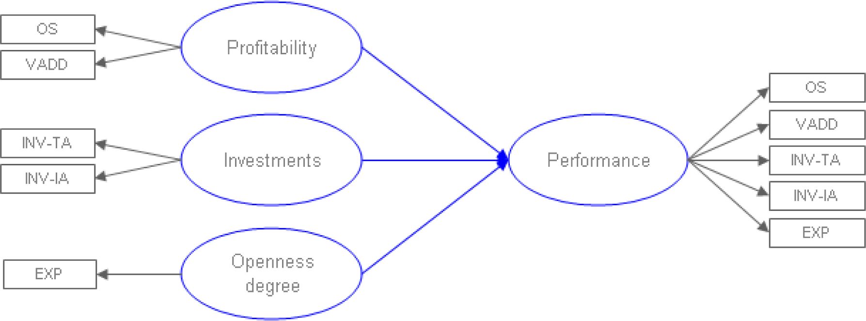
Below we briefly describe formally the method used to estimate the performance indicator and refer to Tenenhaus et al. (2005), Tenenhaus and Esposito Vinzi (2005) for more technical details. The estimated model is shown in Figure 1 by a typical SEM representation, where ellipses represent the latent variables and rectangles the manifest variables, while arrows identify the relationships between them.
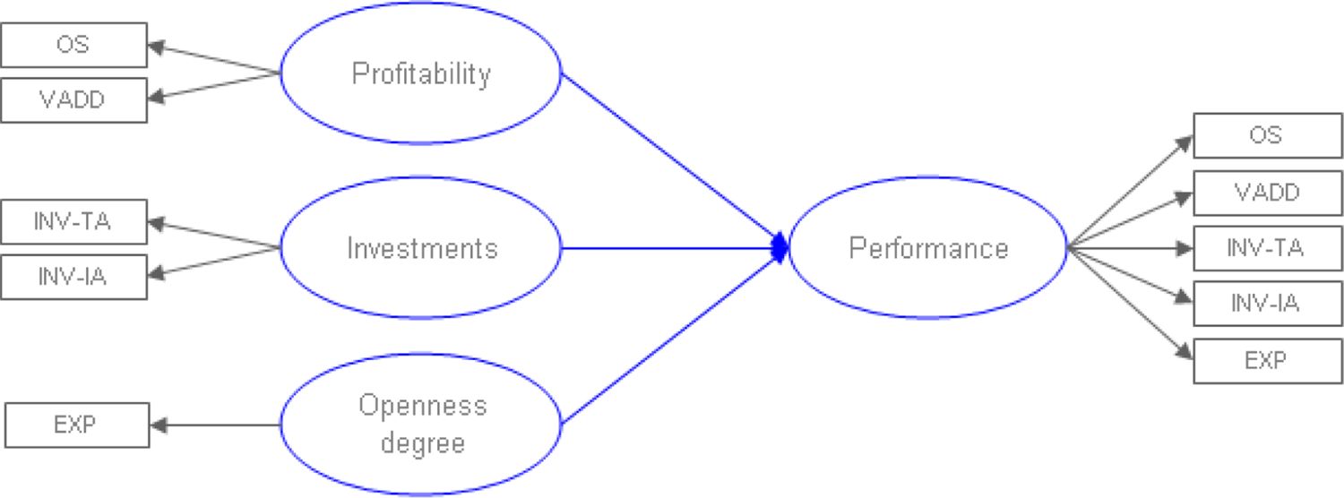
The causal model for performance estimation.
Legend: OS = Operating surplus, VADD = Value added, INV-TA = Investments (tangible assets), INV-IA = Investments (intangible assets), EXP = Turnover from exports
Several specifications with different combinations of manifest and latent variables were considered and estimated. The final one (Figure 1) actually includes basic information on performance factors so that the model structure is simple so as to maintain its validity in terms of both statistical significance of coefficient estimates and relative impact of factors on performance over the three years of analysis, both for large and small and medium-sized enterprises.
In a nutshell, we assume enterprise performance depends on three factors (dimensions): profitability, investments and openness degree that can be observed through the following manifest variables: operating surplus and value added (profitability), investments in tangible/intangible assets (investments), turnover from exports (openness degree). Global performance plays the role of the fourth latent variable, endogenous: it is explained by the three exogenous performance factors and it is observed through the same set of manifest variables describing the first three factors. This is a particular way to specify the model, typical of Multi-block Analysis (Tenenhaus & Esposito Vinzi, 2005).
Among the available approaches to SEM estimation, we use the so-called component-based one. This determines values of the latent variable for each observation in the sample by identifying a latent variable explaining at the same time both its own block of indicators and the relationships between blocks. Among the component-based techniques, the most widely used method is the PLS Path Modeling algorithm (PLS-PM, Wold, 1982; Tenenhaus et al., 2005). PLS-PM does not rely on specific distributional hypothesis. Moreover, it provides systematic convergence of the algorithm, a practical interpretation of the latent variable estimates, and it represents a general framework for multi-block analysis.
We use PLS-PM for SEM estimation of enterprise performance also because we are interested in describing enterprises behaviour, given the model we hypothesized, rather than in testing the validity of the model itself. So the explorative approach is more convenient than the confirmatory one, typical of other approaches to SEM estimation.
PLS-PM is based on an iterative algorithm consisting of a system of multiple and simple regressions, alternated for an inner and outer estimate of the latent variables. This algorithm uses the function PLS-PM of XL-Stat.
Formally, given the generic latent variable ξq, the PLS-PM algorithm iteratively determines:
the outer estimate of the standardized latent variable vq obtained as a linear combination of its own manifest variables xpq, that is
(1)where Pq is the number of manifest variables associated to the q-th latent variable and Wpq represents the outer weights, i.e. the weight associated to each manifest variable to obtain the latent variable estimate;
the inner estimate of each standardized latent variable zq, computed by using its outer estimate of the previous step and considering its relations with the other latent variables. In other words, the inner estimate of each standardized latent variable (ξq − mq) is obtained as;
(2)where, vq’ is a generic latent variable connected to the q-th latent variable, and eqq is the sign of the correlation between the latent variables ξq and ξq';
the outer weights Wpq, measuring the strength of the relationship between each manifest variable and its own latent, to be reused in the next iteration for the outer estimate of the latent variables.
In PLS PM analysis it is also possible to define the direction of the relationship between each manifest variable (MV) and the latent variables (LV) within each block. We assume a reflective scheme, i.e. the latent variable is considered as a predictor of the manifest variables. Thus, each relation in the block is a simple linear regression model 1, i.e. as:
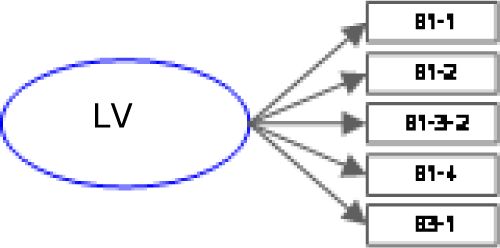
where Wpq is the generic loading (i.e. the correlation coefficient) associated to the p-th manifest variable linked to the q-th latent variable, and εpq is a residual term.
After updating the outer weights they are used to obtain a new outer estimate of the latent variables. These three steps are repeated until convergence between inner and outer estimates. The final estimates of the latent variables are then computed and the structural relations among the latent variable are quantified by standard multiple/simple linear regression models.
For a generic endogenous latent variable in the model, the structural model can be written as:
where ξm is the generic (exogenous or endogenous) latent variable impacting on , bqm is the OLS regression coefficient (pathcoefficient) linking the q-th endogenous latent variable to the m-th latent variable impacting on it, ζq is a residual term, and M is the total number of exogenous latent variables impacting on .
To sum up, for each year considered in the analysis we estimated two models2, one for large enterprises and one for small and medium-sized firms. As already explained, the model also allows us to estimate the weights of the relationships between variables (latent with manifest and latent with latent). These are the regression coefficients of the regression models ruling the influence of the observed variables on the latent variable Performance (i.e. on the performance index). To study the effects of the DIT allowance on enterprise performance we then perform a regression analysis.
As an example of the model output, Table A.1 in the Appendix reports the outer weights estimates for the years 1998–2001, while Table A.2 displays the performance indicator by business sector and firm size (number of employees) for the years 1999, 2000, 2001. Recalling that the performance scores are standardized (i.e. the mean score is 0 for each estimated model), the results must be interpreted with due consideration that positive/negative values are respectively higher/lower than the mean performance.
5. The corporate tax microsimulation model
As explained in Section 3 the DIECOFIS model used in this paper is based on a compound dataset obtained by integrating different sources of data on firms which makes it possible to have a complete representation of the corporate tax system existing in 1998 (large companies) and in the years 1999 and 2000 (both large and small and medium-sized firms). DIECOFIS also simulates social insurance contributions paid by enterprises, a local tax (IRAP), and excises (Bardazzi, Parisi & Pazienza, 2004) for the same years.
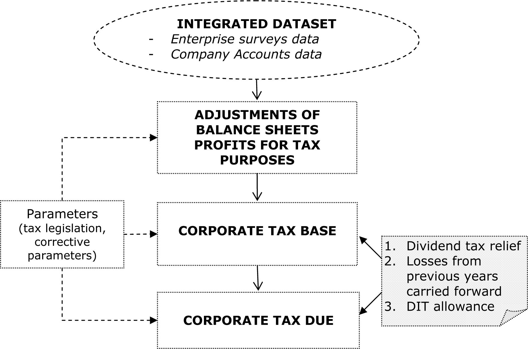
The structure of the model is reported in Fig. 2.
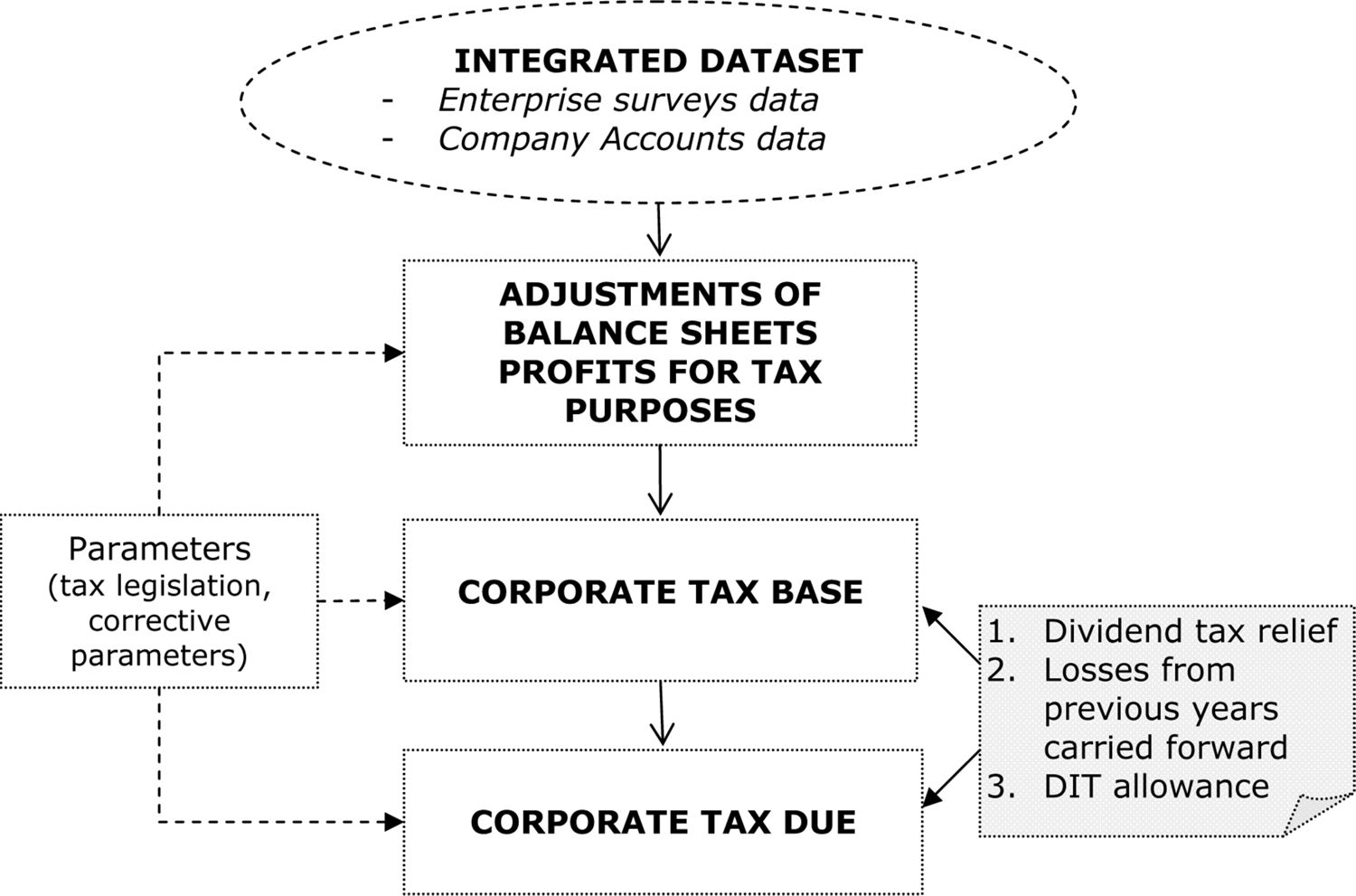
The structure of the corporate tax microsimulation model.
The model is built in Stata and follows a modular structure reflecting the corporate income tax rules described below.
Its main building blocks are the routines Fiscal Adjustments, Corporate Income, Corporate Tax, which run sequentially.
The first two modules (adjustments of balance sheets profits for tax purposes, corporate tax base) compute corporate income for tax purposes. In Italy, as in many other countries, corporate income is obtained from total business profits (losses) shown in company accounts, adjusted according to specific tax rules. These adjustments reflect the difference between the conventional accounting rules and business accounting for tax purposes. Information available in the dataset, and more generally in company accounts, is not detailed enough to simulate tax adjustments of reported profits. The model reproduces tax adjustments of write-down to receivables, amortisation of tangible/intangible assets, and certain expenses, while fiscal adjustments that cannot be modelled on the basis of the available data are “imputed" using parameters computed from the corporate tax returns micro data, available for a sample of firms. These parameters reflect the incidence of the specific adjustments/provisions on some variables (usually reported profits). To improve the accuracy of these corrections, coefficients are computed on a sectoral and dimensional basis.
Once corporate income for tax purposes has been computed, taxable income is obtained by adding the dividend tax credit (given the imputation system subsequently abolished in 2004) to corporate income and by deducting losses from previous periods that can be brought forward up to five years.
The gross tax is calculated by applying the prevailing tax rates to the tax base, and the corporate tax due, or the tax actually paid by the company, is obtained by subtracting the dividend tax credit and the main tax reliefs from the gross tax.
The final output of the module contains the main variables generated within the corporate tax module, i.e. taxable income, allowable DIT income, tax reliefs, gross tax, tax due. At intermediate levels, the model also generates variables reflecting eligible amounts of specific allowances that companies can bring forward to subsequent years, whenever companies do not benefit for the full amount. This is the case of the tax loss for the year, income eligible for the reduced rate under the DIT system, and tax reliefs.
Model output (aggregate amounts, eligibility to the various tax credits, reliefs, and to the DIT allowance) is validated against tax returns micro data, as said available for a sample of firms. Oropallo and Parisi (2007) report a very good fit of the model.
6. Effects of the dit system on enterprise performance
In order to analyse the impact of the DIT allowance we first explore its effects on the company tax burden. To this end we compute average corporate tax rates using the DIECOFIS microsimulation model. As explained the model allows precise computation of effective rates of corporate taxation, known as implicit or ex-post or backward-looking tax rates. Implicit rates relate taxes paid by the company to some aggregate item of the company balance sheet, generally reflecting some “income” concept of the firm, hence a company balance sheet item such as enterprise operating surplus, profits before taxation, turnover. Obviously the magnitude of the figures tends to vary according to the basis of the tax rates. The most immediate item is operating surplus, basically a measure of profits before extraordinary activities and taxes, and in the analysis we choose this base.
As they use ex-post real-life data, they are often described as backward-looking indicators reflecting the fact that measures of effective taxation imply past investment decisions. On the opposite, ex-ante marginal tax rates follow a forward-looking approach focussing on enterprise marginal decisions and are based on computations of the impact of taxes on the cost of capital. Specifically, ex-ante tax rates measure the theoretical tax burden on a hypothetical marginal investment (giving no extra-profits) that produces cash-flow chargeable to tax and, therefore, are calculated to analyse how the tax system affects a marginal investment undertaken by the company, using alternative financial sources. The methodology to derive ex-ante marginal indicators can be also extended to infra-marginal investments, that is investments with different rates of profitability. In the latter case the literature refers to ex-ante average tax rates.
Being simplified measures, forward-looking indicators do not take into account the complexity and the interaction of all elements of the tax system (definition of corporate profits for tax purposes, carry-forward losses provisions, allowances, tax credits and so on) which crucially alter effective company taxation. On the opposite, implicit tax rates can be derived considering the various features of the tax system and therefore give a precise measure of the effective tax burden supported by the firm. Such rates are particularly appropriate if the objective of the analysis is studying the effects of the tax system on enterprise cash flows and to focus on distributional burdens (for instance at sectoral level or on firms of different size).
A comparison of the implicit tax rates in the various years would not be very informative as tax rates change also because of the economic cycle. Under the DIT scheme (see Section 2) the statutory rate ranges between the prevailing rate and the reduced rate, depending on the amount of profits eligible for the allowance (normal profits) on overall profits. Therefore, to focus on the impact of the DIT system, we use DIECOFIS to compare the average tax rates resulting from this regime with the average tax rates simulated under a “standard" system where profits are taxed at the prevailing statutory rate. Obviously this may overestimate the effects of the DIT scheme as, given tax revenue, one could assume the policy maker might have set a lower statutory rate under a single-rate regime.
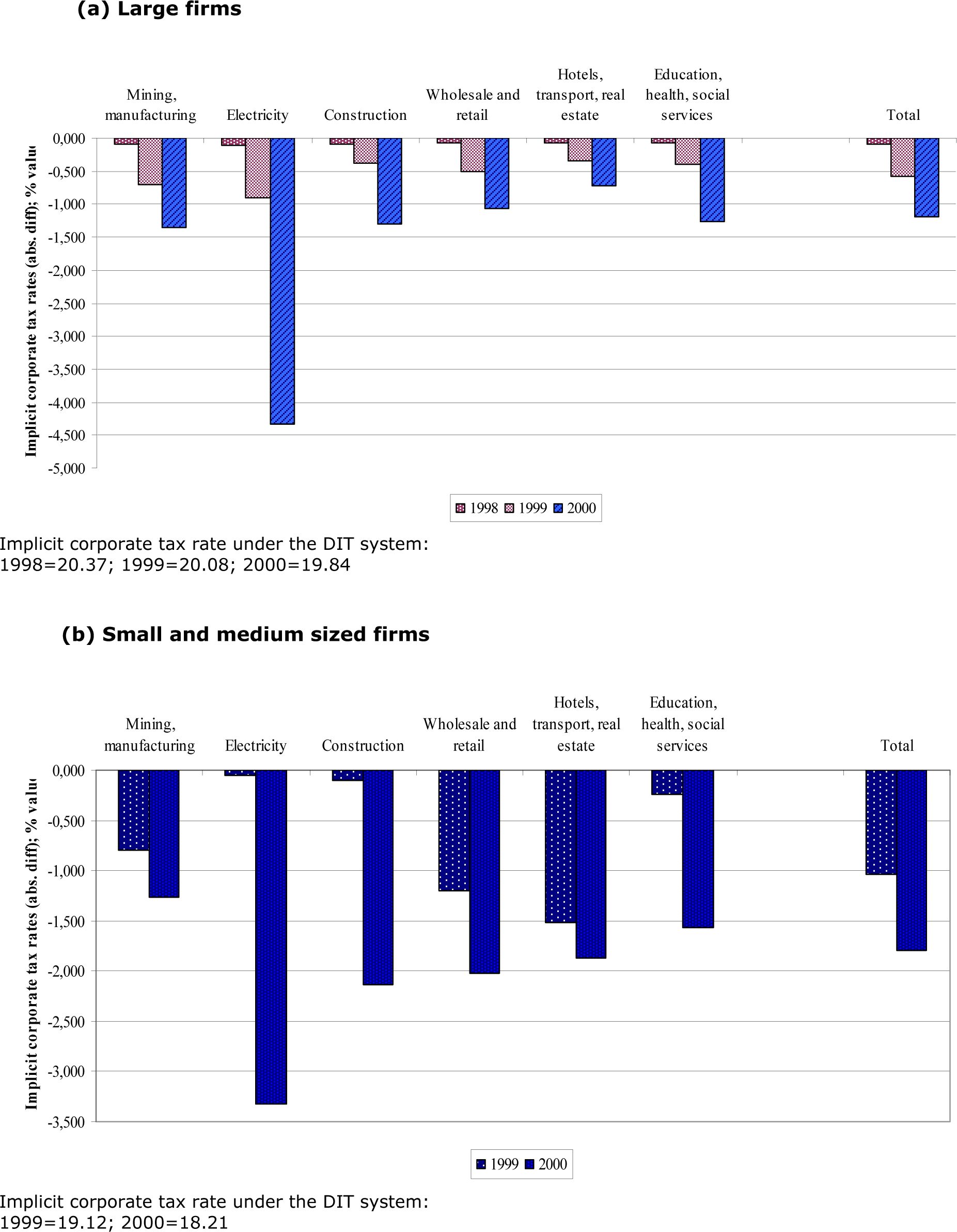
To get a first picture of the impact of the DIT allowance regime, Table 2 reports the simulated number of companies qualifying for this allowance. The number of both large and small-medium sized firms benefiting from the allowance increase in the years considered in the analysis. In 2000 over 50 per cent of the total number of large firms (4,405) and small-medium sized firms (9,772 representing a weighted number of 2,50,826 companies when reported to the universe) benefit from the DIT scheme. This shows a potential strong impact of this regime in reducing the company tax burden. Figures 3(a) and 3(b) report the absolute changes in the implicit tax rates due to the operation of the DIT allowance, by business sector.
Simulated number of companies in the dataset eligible to the DIT allowance. Years 1998–2000.
| 1998 | 1999 | 2000 | ||||
|---|---|---|---|---|---|---|
| Number | % | Number | % | Number | % | |
| Large firms | 3,070 | 37 | 3,692 | 43 | 4,405 | 55 |
| Total | 8,277 | 100 | 8,509 | 100 | 8,009 | 100 |
| Small and medium sized firms | 4,217 | 30 | 9,772 | 54 | ||
| Total | 14,043 | 100 | 18,187 | 100 | ||
-
Source: Authors’ computations

Changes in the implicit corporate tax rates due to the DIT system. Years 1998–2000.
Source: Authors’ computations
The DIT system lowered the average corporate tax rate of both large firms and small-medium sized firms. Tax rate falls are rather modest in 1998 (only 0.08 points for large firms) but increase in 1999 (0.58 and 1.03 respectively for large and small firms) and 2000 (1.20 and 1.80 for large and small firms).
Both in 1999 and 2000 tax rate falls are greater for small and medium sized firms compared to large firms. This result confirms the theoretical prescriptions. Indeed, one expects the incentive to use the DIT allowance to be greater for small firms as they that are generally more debt- constrained and face higher interest rates than larger firms.
Looking at the sectoral effects for instance for the year 2000 we see that the benefits of the DIT scheme are greater in the electricity sector where the implicit rate reduces by 4.34 point (large firms) and 3.32 points (small and medium sized firms), and for small companies in the construction (2.02) and wholesale (2.14) sectors. In the remaining sectors, for companies of both groups, falls of the implicit tax rates are in line with the mean reductions (and amount to about 1 percentage point), while they tend to be smaller for large companies of the hotels, transport real estate sector where the implicit rate declines by 0.73 points.
As said the DIT regime was introduced to reduce the incentive towards debt as a source of finance, as opposed to equity, and at the same time to provide a selective reduction in the burden of taxation.
As the DIT regime lowers the cost of capital of investments financed through equity, its ultimate effect might have been a stimulus to investments. Furthermore, as the debt-equity ratio of Italian non-financial firms at the beginning of the 1990s was the highest among the main European countries (De Bondt, 1998), improvement of the capital structure resulting form the operation of the DIT scheme might have strengthened the competitive position of firms, especially for those more opened towards international markets.
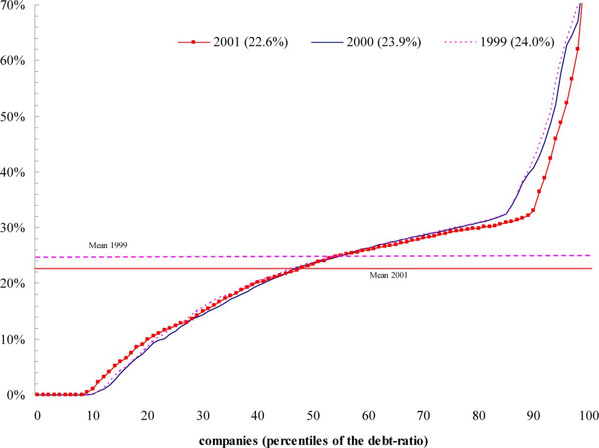
Figure 4 illustrates the change in the debt-ratio (calculated as the share of financial debts over firm net assets) for companies of our dataset in the years 1999–2001. Firms are ordered by percentiles of the debt-ratio.

Debt-ratio (financial debts/net assets); years 1999–2001.
Source: authors’ computations on ISTAT data The average debt-ratio fell by 1.4 percentage points in the period 1999–2001, and this suggests a significant effect of the DIT mechanism on firms’ capitalisation3.
Given the theoretical reasons discussed above, we assume that qualifying for the DIT allowance at time t may influence firm performance at time t +1. In this case we can assume causality following the adagium that cause (being eligible to the DIT) precedes consequence (performing “better"). Therefore we perform regression analysis using a dummy variable identifying companies benefiting (DIT=1) and not benefiting (DIT=0) from the DIT allowance in each year. The dependent variable is represented by the estimated performance index (in the subsequent year).
The analysis is carried out for the years 1999–2001 for large companies and for the years 2000–2001 for small and medium sized firms and the results are reported in Table 3 and 4. It is important to note that as the dataset covers a sample of small and medium sized firms, regressions for this group are performed on the sub-sample of firms present for two subsequent years, numbering to 3,410 units in 1999–2000 and to 3,708 units in 2000–2001. Being the sampling procedures in different years independent, these sub-samples keep the characteristics of random samples.
Regression analysis: average performance (years 1999, 2000, 2001) of companies not benefiting (DIT=0), benefiting (DIT=1) from DIT in the previous year. Large firms.
| 1999 | 2000 | 2001 | |||||||
|---|---|---|---|---|---|---|---|---|---|
| Value | t | Pr>| t | | Value | t | Pr>| t | | Value | T | Pr>| t | | |
| < | < | ||||||||
| Intercept | 0.000 | 474.755 | 0,0001 | 0.000 | 201.248 | 0,0001 | 0.000 | 167.450 | < 0,0001 |
| < | < | ||||||||
| DIT=0 | 8.083 | 376.577 | 0.0001 | 5.164 | 188.882 | 0.0001 | 3.235 | 57.039 | < 0.0001 |
| < | < | ||||||||
| DIT=1 | 8.147 | 474.755 | 0.0001 | 5.234 | 201.248 | 0.0001 | 3.183 | 167.450 | < 0.0001 |
Regression analysis: average performance (years 2000, 2001) of companies not benefiting (DIT=0), benefiting (DIT=1) from DIT in the previous year. Small and medium sized firms.
| 2000 | 2001 | |||||
|---|---|---|---|---|---|---|
| Value | t | Pr>| t | | Value | T | Pr>| t | | |
| Intercept | 0.000 | 946.448 | < 0.0001 | 0.000 | 912.961 | < 0.0001 |
| DIT=0 | 8.356 | 634.464 | < 0.0001 | 8.468 | 351.932 | < 0.0001 |
| DIT=1 | 8.827 | 946.448 | < 0.0001 | 8.507 | 912.961 | < 0.0001 |
-
Source: Authors’ computations
Having fixed the value of the intercept to 0, the regression coefficients are equal to the mean performance of the two groups. As performance scores in each year and for large, small-medium sized companies have been estimated by independent models, performance values cannot be compared neither through years nor between the two groups.
The coefficients are always statistically significant. To make comparisons more immediate, the highest value in each year is in bold. With the exception of 2001 for the group of large firms, on which we return below, results show clearly that companies qualifying for the DIT allowance (in the following year) perform better than companies not benefiting from this regime. This result holds for 1999 and 2000 for large companies (compare 8.147 with 8.083, and 5.234 with 5.164), as well as for small-medium sized firms both in 2000 and 2001 (compare 8.827 with 8.356, 8.507 with 8.468).
As said, by contrast, in 2001 large companies that did not benefit from the DIT in the previous year perform better than firms qualifying for the allowance (compare 3.235 and 3.183). This result must be taken with due caution as it is most likely due to the economic cycle. Indeed, as the estimates of the performance index (see Table A.2 in the appendix) indicate for 2001, firms with 100 or more employees exhibit a negative outcome in terms of global performance (performance values range from -1.61 for the class with more than 999 workers to -3.838 for companies with a number of workers between 100 and 249). Furthermore, the manufacturing and the hotels, transport, real estate sectors than on the whole cover about 70% of the total number of corporations, record negative performance (respectively -0.071 and - 0.227) and obviously this result is due to larger rather than small and medium sized firms.
For the group of large corporations it must have been the case that in 2001 the negative economic cycle involved at a greater extend companies that had benefited from the DIT allowance compared to firms that did not qualify for this scheme.
In conclusion the analysis demonstrates that the DIT regime had a generally positive impact on enterprise performance4 in the sense that firms benefiting from this regime outperformed non eligible companies. This result is somehow in line with the empirical results of other studies that find a positive effect of an ACE on investment (see Klemm, 2007).
7. Conclusions
In this paper we have explored the effects of the Dual Income Tax introduced in Italy in the period 1998–2001, on enterprise performance.
This analysis is innovative as empirical evaluations of the ACE systems have generally focused on their impact on the firm tax burden and the distortion on company financing choices (for a review see Klemm, 2007), but there is little evidence of the effects of these reforms on enterprise performance.
Enterprise performance is a complex concept where performance can be viewed as being dependent on factors or dimensions that cannot be measured directly, but can be observed as a reflection of a set of observable indicators of enterprise activity. In this paper we assume company performance is explained through three dimensions, namely profitability, investments, openness degree, that can be observed through the following manifest variables: operating surplus and value added, investments in tangible/intangible assets, turnover from exports. In order to compute a composite indicator we estimated a SEM where the performance factors and performance itself played the role of latent variables while the observed indicators were manifest variables. The model was estimated using the PLSPM approach to SEM (Wold, 1982). Enterprise performance is computed on a compound dataset combining company balance sheets with Italy’s Institute for Statistics (ISTAT) enterprise survey data. The data cover for the period 1998–2001 the universe of large firms (with 100 or more employees) and a representative sample of small and medium-sized companies (with fewer than 100 employees). Companies in the banking and agricultural sectors are excluded from the analysis.
To study the effects of the DIT allowance on company performance, on the assumption that qualifying for the DIT allowance at time t may benefit firm performance at time t +1, we perform regression analysis where the dependent variable is represented by the estimated performance index and the explicative variable is a dummy identifying companies qualifying or not qualifying for the DIT allowance. This analysis is carried out for the years 1998–2001 for large companies and for the years 1999–2001 for small and medium sized firms.
Eligibility to the DIT allowance is simulated by means of the DIECOFIS corporate tax model. Using the compound dataset makes it possible to simulate in detail the various elements of the corporate tax system (computation of the tax base, application of the various tax credits, reliefs), and obviously the operation of the DIT system.
The empirical analysis shows that the DIT allowance positively affected firm performance, as defined on the basis of the specified factors. Indeed the coefficient of the regression analysis, the mean performance, of companies qualifying for the DIT is always greater than the coefficient estimated for non-eligible companies. The only exception is represented by the year 2001 for the group of large companies, when we actually obtain the opposite result. However, this result is most likely due to the negative economic cycle that evidently affected at a greater extend companies that benefited from the DIT compared to the group of firms not eligible to this regime. The results are in line with the theoretical expectations as reduction of the cost of capital of investment financed through equity capital, improvement of the company financial structure, reduction of the effective rate of taxation, all provided by the DIT system, operate in the sense of increasing company performance.
The analysis does not allow to disentangle the effect of each single factor. Therefore it is difficult to say whether the positive effect on performance was mainly due to the reduction of the effective rate of taxation or to company investments. If the first effect dominates, from the policy maker’s point of view one could assume that a general cut of the statutory rate under a standard corporate tax system could have had similar effects on enterprise performance through its impact on firm profitability. However, we again emphasize the efficiency features of the DIT regime compared to a standard one and its selective nature: a DIT system incorporates an incentive to increase capitalization in order to qualify for the reduced rate of taxation and this appears crucial for the Italy’s corporate sector where the debt-equity ratio is very high also by international standards (De Bondt, 1998).
From this perspective the DIT reform can be judged positively as it actually addressed one specific weakness of the Italy’s corporate sector while offering at the same time an economic stimulus to firms that increased capitalization.
Footnotes
1.
By contrast, in the formative scheme the latent variable is a function of its own indicators. In this case each block is a multiple linear regression model.
2.
The model assessment results are not discussed here. However, it must be emphasized that all latent variables have a significant and positive impact on the performance variable.
3.
Though financial debts are generally higher for large companies compared to small-medium sized ones, the ratio of debts on company net assets actually decrease by firm size. Figure 4 reveals that the decline of the debt-ratio was especially strong for companies of upper percentiles (small and medium sized firms), whereas this ratio even increased for lower percentiles (larger firms), and this confirms that the impact of DIT was stronger for small and medium sized firms.
4.
Also, we recall that in the same years a temporary incentive for investments financed through equity capital was introduced (see Section 2). Therefore it might also be the case that firms qualifying for the DIT allowance benefited also from this incentive which indeed reinforced the effects of the DIT on investments.
Appendix
Weight of performance factors; 1998–2001.
| Large firms | Small and medium sized firms | |||||||
|---|---|---|---|---|---|---|---|---|
| 1998 | 1999 | 2000 | 2001 | 1999 | 2000 | 2001 | ||
| PERFORMANCE | Operating surplus | 0.831 | 0.823 | 0.829 | 0.847 | 0.750 | 0.742 | 0.884 |
| Value added | 0.936 | 0.901 | 0.882 | 0.879 | 0.825 | 0.781 | 0.895 | |
| Investments (tangible assets) | 0.936 | 0.961 | 0.902 | 0.881 | 0.381 | 0.339 | 0.325 | |
| Investments (intangible assets) | 0.213 | 0.716 | 0.574 | 0.473 | 0.385 | 0.341 | 0.326 | |
| Turnover from exports | 0.399 | 0.346 | 0.444 | 0.474 | 0.592 | 0.573 | 0.415 | |
-
Source: Authors’ computations.
Enterprise performance (standardized values) by business sector, firm size; years 1999, 200, 2001.
| 1999 | 2000 | 2001 | N % (2001) | |
|---|---|---|---|---|
| Business sector | ||||
| Mining, manufacturing | 0.263 | 0.200 | −0.071 | 47.97 |
| Electricity | 0.229 | 0.242 | 2.076 | 1.24 |
| Construction | −0.114 | −0.082 | −0.651 | 3.43 |
| Wholesale and retail | −0.029 | −0.011 | 0,372 | 14.87 |
| Hotels, transport, real estate | −0.073 | −0.071 | −0.227 | 24.35 |
| Education, health, social services | −0.125 | −0.075 | 0,174 | 8,14 |
| Firm size (number of employees) | ||||
| 1-19 | −0.097 | −0.078 | 1.424 | 39.33 |
| 20-49 | 0.613 | 0.437 | 1.839 | 16.57 |
| 50-99 | 1.886 | 1.339 | 2.006 | 16.68 |
| 100-249 | 0.111 | 0.053 | −3.838 | 18.42 |
| 250-499 | −0.035 | −0.029 | −3.712 | 5.45 |
| 500-999 | 0.105 | 0.314 | −3.492 | 2,08 |
| more than 999 | 1.710 | 1.958 | −1.610 | 1.47 |
-
Source: Authors’ computations.
References
-
1
Completeness of Information and Imputation from Donor with Minimum Mixed DistanceQuaderni di Ricerca ISTAT, n4.
-
2
Modelling direct and indirect taxes on firms: a policy simulationAustrian Journal of Statistics 33:237–259.
-
3
A General Proposition on the Design of Neutral Business TaxJournal of Public Economics 24:231–239.
-
4
Reforming Business Taxation: Lessons from Italy?International Tax and Public Finance 8:191–210.
-
5
Financial Structure: Theories and stylized facts for six EU CountriesDe Economist 146:271–301.
- 6
- 7
- 8
- 9
-
10
Handbook on constructing composite indicators: methodology and user guide. OECD Statistics Working PaperHandbook on constructing composite indicators: methodology and user guide. OECD Statistics Working Paper.
-
11
Will Italy’s Tax Reform Reduce the Corporate Tax Burden? A Microsimulation AnalysisRivista di Statistica Ufficiale 1:31–55.
-
12
International Research into Developing Integrated and Systematized Information Systems (Elsis) for EU Business Policy Impact AnalysisAustrian Journal of Statistics 33:3–33.
- 13
-
14
PLS regression. PLS path modeling and generalized Procrustean analysis: a combined approach for multi-block analysisJournal of Chemometrics 19:145–153.
-
15
Systems under indirect observation, North-Holland, Amsterdam1–54, Soft modeling. The basic design and some extensions, Systems under indirect observation, North-Holland, Amsterdam.
Article and author information
Author details
Publication history
- Version of Record published: August 31, 2011 (version 1)
Copyright
© 2011, Balzano et al.
This article is distributed under the terms of the Creative Commons Attribution License, which permits unrestricted use and redistribution provided that the original author and source are credited.