Developing a static microsimulation model for the analysis of housing taxation in Italy
- University of Torino, Italy
- Article
- Figures and data
- Jump to
Abstract
In this paper we develop the first (static) microsimulation model aimed at studying the distributive impact of housing taxation on Italian households. We use as input data those provided by the Bank of Italy from its Survey on Households Income and Wealth, and discuss specific problems arising in the evaluation of cadastral income and of the Property Tax base. Our estimates of the distribution of taxpayers are very close to the Ministry of Finance official statistics; hence, our model can be seen as a reliable tool to evaluate the current distribution of housing taxation and the impact of potential tax reforms. Our simulations suggest that both Property Tax and Waste Management Tax show a moderate regressive impact with respect to household gross income, whilst the Personal Income Tax on dwellings other than the main residence is progressive. We then provide an application of our model, to study the Property Tax reform in 2008. Our findings show that all households owning the main residence gain from the 2008 reform, but tax cuts are mostly concentrated on the top three deciles of household equivalent gross income, so that the richest benefit most.
1. Introduction
Despite the importance of housing in influencing citizens’ well-being, the large share that housing represents in citizens’ wealth, and the large share of income devoted to expenditures for its maintenance, housing taxation is an understudied topic that deserves more attention, both from a positive and a normative perspective. For instance, from a positive perspective, questions arise in order to explain the current distribution of housing taxes and how they impact on the distribution of resources; from a normative point of view, it is important to understand how an ’optimal tax’ on housing can be designed.
The absence of almost any study on the issue of housing taxation is magnified in the case of countries where taxes have been used – together with other policies – to favour homeownership. Italy is an important case study in this respect for many reasons. Like in other Mediterranean countries (e.g., Spain), the Italian Tax Code basically exempts the figurative income from homeownership, while contemporaneously allowing for tax credits in the case of mortgage interests, creating a clear favour for owner-occupiers (e.g., Baldini, 2010). These fiscal advantages for home-owners reasonably increased given the international trends in market prices, which – differently from tax bases – soared in recent years. Moreover, differently from other countries, Italy shares with the Mediterranean countries also a high number of owner-occupiers coupled with a system of public pensions particularly generous, generating a substantial redistribution in favour of the elderly (e.g., Ferrera and Castles, 1996). In particular, the share of owner-occupied housing has increased strongly since 1977, reaching 72% of Italian households in the late 2000s, a figure close to that of Portugal (73%), but lower than Spain (83%); the share of owner-occupiers is instead lower in Continental European countries, like France and Germany, where these percentages amount to 58 and 46, respectively (e.g., Baldini, 2010). All these redistributive issues are coupled with increasing difficulties for those who do not own their house to afford housing expenses. On the one hand, public expenditures for housing represent only a mere 0.1 percent of welfare expenditures in Italy, compared with an average 3.5 percent in the EU countries (e.g., D’Alessio and Gambacorta, 2007; Baldini, 2010). On the other hand, given the increase in market values and the liberalization of rental markets occurred during the 1990s (with the removal of upper limits), also rents increased noticeably. Hence, the non-owners found it increasingly difficult to buy a house or pay a rent, a situation that could be improved also by reforming housing taxation.
However, no government has tried to propose a general reform of housing taxation to ameliorate the current situation, since the share of owners is high and the issue is politically sensitive. Not surprisingly, a recent reform of the Property Tax, implemented in 2008, increased even further advantages for owners, reasonably creating adverse redistributive effects in order to gain short-term political benefits. Unfortunately, the Italian government has not developed so far a model to assess the distribution of housing taxes, so that fiscal policy simulations are difficult to estimate.
The aim of this paper is to fill the gap, by developing the first (static) microsimulation model explicitly devoted to the analysis of housing taxation in Italy. In particular, we are interested in two basic issues: first, we want to characterize the current distribution of taxes on housing, reconciling the (scant) aggregate figures on housing with those originating from micro data; second, we want to apply the microsimulation model to study the redistributive impact of fiscal reforms, and take the 2008 reform of the Property Tax as a case study. We use as input data those provided by the Bank of Italy from its Survey on Households Income and Wealth, and discuss the specific problems arising in the evaluation of the cadastral income and the Property Tax base. The model replicates fairly well the distribution of taxpayers provided by the Ministry of Finance, which makes it a reliable tool to evaluate tax reforms on housing in Italy. Our simulations on the 2006 data suggest that both Property Tax and Waste Management Tax show a moderate regressive impact with respect to household gross income, whilst the Personal Income Tax on dwellings other than the main residence is progressive. Moreover, studying the Property Tax reform in 2008, our simulations show that all households owning the main residence gain from the 2008 reform, but tax cuts are mostly concentrated on the top three deciles of household gross income, so that the richest benefited most.
The remainder of the paper is structured as follows. Section 2 provides a brief institutional description of housing taxation in Italy. Section 3 describes the microsimulation model, discussing the distribution of cadastral incomes and the simulations of main taxes on houses for Italian households. Section 4 offers a first application of the model, to study the distributive impact of the 2008 reform of the Property Tax. Section 5 briefly ends the paper.
2. Housing taxation in italy: institutional details
Like in other developed countries, there are a number of different taxes on houses and buildings in the Italian tax legislation. Total tax revenues from housing amount to about 40 billion of euro in the late 2000s, i.e. 2.7 percent of GDP and 5.9 percent of total tax revenues (Ministry of Finance, 2008). We can classify ‘housing taxes’ in two broad groups: a first group is identified by taxes on house ownership and dwelling utilization (54% of revenues); a second group considers taxes due when buying or selling, as well as restructuring a dwelling or any other kind of building (46% of revenues). Since our aim here is to develop a static microsimulation model for the analysis of housing taxation, we focus on the first group of taxes only, and limit our analysis to households, leaving aside buildings owned by (public and private) firms. The main taxes of the first group are: the Personal Income Tax (hereafter House- PIT), within which the (figurative) income from houses is taxed (about 7 billion euro); the Property Tax (hereafter ICI, from Imposta Comunale sugli Immobili, Municipal Tax on Buildings, about 5.2 billion euro that dropped to 2.4 billion after the 2008 ICI reform); and the Urban Waste Management Tax (hereafter TARSU, from Tassa per lo Smaltimento dei Rifiuti Solidi Urbani, about 3 billion euro). In what follows we briefly describe the institutional details of House- PIT, ICI and TARSU.
House-PIT
Incomes from dwellings are determined in different ways according to the kind of use, and imputed to each owner or life-tenant1 according to her percentage of ownership. Current rules in the Tax Code identify income for the taxpayer dwelling as the ‘cadastral income’, i.e. a hypothetical rent based on the property description and valuation listed in the local Land Register (the so-called Catasto Fabbricati), which was last revised in 1939 and is clearly far from current market values. Income from unoccupied or holiday homes is equal to cadastral income augmented by one third. Finally, income from rented dwellings is equal to 85 percent of the actual rent. As for the owners, from 2001 onwards the income from the main residence is exempted from the PIT tax base; on the contrary, income from other dwellings is included in the taxable income. Mortgage interests and maintenance expenditures allow the owner a tax credit. As for the renters, up to 2008 no tax credits were allowed for the main residence. At present, a tax credit related to personal income of the renter (up to about 30,000 euro) is allowed; it is higher for renters younger than 30 years old.
ICI
Since 1993 a Property Tax (ICI) on each dwelling has been introduced. The tax unit is the individual according to her percentage of ownership. Tax revenues accrue directly to each Municipality where the buildings are located. In principle, the ICI tax base should be the market value of the dwelling; in practice, this is not the case since it is evaluated by simply multiplying the cadastral income by 1002. Each Municipality can choose the tax rate in a range between a minimum of 0.4 percent and a maximum of 0.7 (Pellegrino, 2007, for further details). Up to 2007, a tax credit on the main residence was available. Starting from 2008, no ICI is due on the main residence
TARSU
Waste management services are financed by a tax directly accruing to municipalities that manage the service. The taxpayers are the households living in the dwellings (regardless of their tenure status), and those owning unoccupied or holiday homes. Contrary to what one could expect, the tax debt is not related to the amount of waste produced by each household, but to the size of the house. In particular, tax debt is determined by multiplying a tariff per square meter by the total surface of the dwelling. Some tax reductions are allowed for people living alone, unoccupied dwellings, and poor households.
3. The microsimulation model
The microsimulation model used in this paper estimates the most important taxes and contributions characterizing the Italian fiscal system, concentrating in particular on the main taxes on housing. This marks a striking difference with respect to other comparable tax-benefit models, like EUROMOD, used to study for instance the impact of the mortgage interest tax relief within the PIT, but with no clear focus on taxes on houses and buildings (e.g., Matsaganis and Flevotomou, 2007). The model considers as input data those provided by the Bank of Italy (2008) in its Survey on Households Income and Wealth (hereafter SHIW-BI). The Survey contains information on household income and wealth in the year 2006, covering 7,768 households, and 19,848 individuals. The sample is representative for the Italian population3, composed by about 23,5 million households and 60 million individuals. Relevant information for the analysis of housing taxation in the SHIW-BI include: the overall net income, the market value of real estates, the size (in square meters) of the dwellings, the dwelling maintenance expenditures, the interests paid on mortgage, and the initial mortgage debt. Notice that the SHIW-BI net income is defined on a personal basis, while mortgage interests and real estates information are available only at the household level. However, by exploiting information on the ownership shares, it is possible to evaluate the value of real estates also at the individual level. We then start by simulating income and taxes at the individual level, and then aggregate results at the household level.
In 2006 the National Land Agency (2008) estimated the total number of residence dwellings to be 30.8 million: 26.2 million (85 percent) are owned by households, while the remaining 4.6 million (15 percent) are owned by public and private firms. This is the only available information at the aggregate level on real estates in Italy, since the National Land Agency statistics refer only to dwelling characteristics and not also to dwelling owners. In what follows we clearly limit our analysis to the 26.2 million of dwellings owned by households.
There are a number of problems to be solved in order to appropriately simulate housing taxation starting from SHIW-BI. First, we need to calibrate the model, attributing second homes to households in order to make SHIW-BI data compatible with aggregate statistics provided by the Ministry of Finance and the Land Register. Second, we need to evaluate cadastral values for given current market values. Third, we need to reconstruct gross incomes starting from net incomes provided in the survey. Fourth, we need to aggregate incomes at the household level, and define an equivalent income for the redistributive analysis. Below, we will discuss solutions for each of these problems.
Table 1 shows the composition of households by tenure status focusing on main residences p>according to the SHIW-BI. Total households are about 23.5 million: 16.1 million (68.7 percent) are the owner-occupiers of their main residence4; 0.7 million (3.1 percent) are life-tenants; 5 million (21.3 percent) rent or occupy it under “redemption agreement" (the so-called "a riscatto”), while 1.6 million (7.0 percent) are rent- free tenants (and in 92 percent of the cases, the dwelling is owned by relatives or friends)5.
Even if the number and the composition of main residences are reliable, the SHIW-BI dataset underestimates the total number of dwellings other than the main residence. In particular, about 3.5 million households (hence 3.5 million dwellings) declare to rent the main residence from other households, while the dwellings the interviewees declare to rent to other households are about 0.8 million; the gap is 2.7 million dwellings. Similarly, about 1.5 million households (1.5 million dwellings) declare to be rent-free tenants, while the dwellings the interviewees declare to rent free of charge to other households are about 0.5 million; the gap is 1 million dwellings. Finally, in the SHIW-BI dataset there are only 2.2 million unoccupied dwellings or holiday homes, while they are expected to be twice as many, as this number is computed by subtracting from the total number of dwellings all the other categories previously analyzed.
Households main residences composition by tenure status.
| Tenure Status | Composition (%) |
|---|---|
| Owner occupiers (with or without mortgage) | 68.7 |
| Life-tenants | 3.1 |
| Tenants or occupiers under redemption agreement | 21.3 |
| Rent-free tenants | 7.0 |
| Total | 100.0 |
-
Note: The total number of households is 2,34,81,999.
-
Source: Own calculations based on SHIW-BI.
There are two possible explanations for the underestimation of the number of dwellings in SHIW-BI: first, the interviewees do not declare the exact number of unoccupied dwellings or holiday homes and rented dwellings, as well as dwellings rented free of charge (Coromaldi & Guerrera, 2009); second, it is not guaranteed that the original SHIW-BI sample contains a representative sub-sample of Italian households owning dwellings other than the main residence. Since SHIW-BI information on the number and on the characteristics of the main residences is reliable, we use this information in order to reconcile the number of dwellings other than the main residence owned by households with aggregate statistics published by the National Land Agency. This calibration is important to obtain a reliable estimation of revenues from housing taxes, and to correctly evaluate the distribution of housing taxation among households. In order to solve the problem, we then consider the whole SHIW-BI sub-sample of households owning at least the main residence and randomly attribute the missing dwellings. Excluding owner occupied dwellings (16.1 million), our estimates suggest that the total number of other dwellings owned by households is about 10 million. Table 2 reports the estimated composition by type of utilization: 0.7 million (6.8 percent) are used by life-tenants, 3.5 million (35 percent) are rented to other families, 1.5 million (14.9 percent) are given up free of charge, while the unoccupied dwelling and holiday homes are 4.3 million (43.3 percent).
Composition of second homes owned by households by type of utilization.
| Type of utilization | Composition (%) |
|---|---|
| Life-tenants households | 6.8 |
| Free-rented to households | 14.9 |
| Rented to households | 35.0 |
| Unoccupied dwellings or holiday homes | 43.3 |
| Total | 100.0 |
-
Note: The total number of dwellings is 1,00,52,261.
-
Source: Own calculations based on SHIW-BI.
Once the number and the composition of dwellings owned by households have been properly estimated, another problem needs to be solved in order to correctly analyze housing taxation through our microsimulation model. This is the estimation of the cadastral value and the cadastral income of each dwelling. This is important since it represents the ICI and House-PIT tax base, respectively, to be imputed to each taxpayer. The National Land Agency estimates the number and the composition, as well as the overall cadastral value of dwellings (i.e., the overall ICI tax base). The SHIW-BI dataset contains information on the current market value of each dwelling owned by households. We compare these two aggregate values in order to obtain the average underestimation of overall cadastral values with respect to overall market values. Then, we impute the same percentage of underestimation (which is approximately equal to 77 percent) to the current value of each dwelling declared by each interviewee. By dividing the result by 100, and using the percentage of ownership of each person within the household, we obtain the cadastral income included in each taxpayer’s definition of PIT gross income. No specific problems arise in the simulation of TARSU, since it is linked to the size of the dwelling.
Once incomes from housing have been identified, as the SHIW-BI provides information on each individual net income, we need to estimate the gross income for each taxpayer. Since the SHIW- BI definition of each individual net income is different from the Tax Code definition, the microsimulation model first distinguishes all incomes included in the PIT taxable income definition, incomes exempt from any taxes, and incomes taxed under a separate regime. The PIT gross income distribution is then evaluated starting from the net income distribution. The transition from the post- to the pre-tax personal income of each individual has been computed by applying the algorithm proposed by Immervoll and O’Donoghue (2001). Using original sample weights, the grossing-up procedure simply proportions the sum of individuals’ sample weights to the dimension of the population as estimated by the National Statistical Office (ISTAT). Then the grossed-up number of PIT taxpayers has been obtained by considering individuals with a positive gross income within the microsimulation model.
Finally, we aggregate net and gross incomes at the household level. The gross income is equal to the sum of PIT gross income, family benefits (the so-called Assegni al Nucleo Familiare, a small cash transfer varying with the number of children and income), incomes exempt from taxation, gross incomes from financial assets, gross incomes taxed under a separate regime. The net income is equal to the gross income net of all taxes considered in the model: PIT, taxes on financial assets, taxes due on income taxed under a separate regime, ICI, TARSU, and IRAP (the regional tax on the value added). We subtract the mortgage interests from the result. In the following analysis, we consider all households in the dataset; in particular, we do not drop households with zero household income in order to obtain results on a homogeneous sample. In order to obtain the equivalent income we adopt the Cutler Scale (CS), defined as:
where 0 ≤ NA ≤ 1 and 0 ≤ NC ≤ 1 are, respectively, the number of adults and children6 within each household, whilst 0 ≤ α ≤ 1 is the parameter assigning a different weight to children with respect to adults, and 0 ≤ β ≤ 1 indicates the ‘scale economies’ attached to the equivalence scale7.
4. Simulation results
In this section we discuss the results of our simulation exercise of the main taxes on housing. We begin by comparing statistics from our model with official statistics, and then describe the main findings from the simulation.
In order to assess the “goodness – of-fit” of the model, we compare our results with the Ministry of Finance official statistics. Unfortunately, statistics on House-PIT are available only at the individual level, while no official statistics on ICI and TARSU distribution have been ever published. As a consequence, we first compare the PIT module results of the microsimulation by considering the individual as the reference tax unit; we then discuss results at the household level.
Table 3 presents the differences between the simulation results and the official statistics from the Ministry of Finance, in terms of numbers of taxpayers and average gross income. As can be concluded from the table, differences are proportionally very small.
Notice that only statistics on employees and pensioners (who represent 87.1 per cent of the overall taxpayers), as well as self-employed taxpayers are fully comparable, since the Ministry of Finance official statistics do not specifically focus on taxpayers having only other kind of incomes (e.g., only income from dwellings).
The estimated number of employees and pensioners within the microsimulation model is, respectively, 0.5 and 0.3 percent lower than the official figure, while the number of self-employed taxpayers is 4.4 percent higher. On the contrary, the estimated number of ‘other’ (non working) taxpayers appears to be substantially different from official statistics (81.6 percent higher). The explanation of this huge difference is quite simple: by considering all observations within the SHIW dataset, the microsimulation model is able to identify all taxpayers with a positive gross income, while official statistics cannot consider taxpayers for whom the tax return form presentation is not compulsory according to Italian rules; this happens for instance when taxpayer’s gross income is represented by the main residence cadastral income only.
Table 4 presents the PIT gross income distribution by income classes. Again, official statistics are very close to our estimates. Some differences can be observed only for the number of taxpayers belonging to the classes 0–3, 15–20 and 29–40 thousands euro.
Given the good approximation of the model, we now discuss simulation results on ‘housing taxes’ more in detail. We start from the estimates of cadastral incomes. About 16.8 million of households own the dwelling where they live. According to the SHIW-BI dataset, about 50 percent of main residences are owned only by one individual, while the other 50 percent have two or more owners. As a consequence, PIT taxpayers with a positive main residence cadastral income are about 24.3 million (40.5 percent of the population).
Composition of PIT taxpayers and mean gross income by work status.
| Year 2006 | Number of taxpayers | Mean gross income (euro) | ||||
|---|---|---|---|---|---|---|
| Work status | Microsimulation model (A) | Ministry of Finance official statistics (B) | (A)/(B) | Microsimulation model (C) | Ministry of Finance official statistics (D) | (C)/(D) |
| Employee | 1,97,90,570 | 1,98,98,390 | 99.5 | 21,121 | 21,229 | 99.5 |
| Pensioner | 1,52,82,140 | 1,53,29,420 | 99.7 | 15,717 | 16,103 | 97.6 |
| Self employed | 41,65,622 | 39,89,143(a) | 104.4 | 18,768 | 18,697(b) | 100.4 |
| Other taxpayer | 22,55,637 | 12,41,749(c) | 181.6 | 2,063 | - | - |
| Total | 4,14,93,969 | 4,04,58,702 | 102.6 | 17,858 | 18,324 | 97.5 |
-
(a)
The statistic considers taxpayers with VAT code.
-
(b)
The number of these taxpayers has been evaluated as difference.
-
(c)
The mean value has been obtained considering taxpayers with positive and negative incomes.
-
Source: Own calculations based on SHIW-BI and Ministry of Finance 2008.
Gross income distribution by income classes (all taxpayers).
| Year 2006 | Microsimulation model | Ministry of Finance official statistics | ||
|---|---|---|---|---|
| Income class (euro) | Composition (%) | Mean (euro) | Composition (%) | Mean (euro) |
| 0–1.000 | 6.8 | 344 | 5.0 | 453 |
| 1.000–3.000 | 3.7 | 2,000 | 5.1 | 1,934 |
| 3.000–5.000 | 3.7 | 4,065 | 4.1 | 3,998 |
| 5.000–7.500 | 11.7 | 6,243 | 12.2 | 6,093 |
| 7.500–10.000 | 6.9 | 9,037 | 8.3 | 12,365 |
| 10.000–15.000 | 17.9 | 12,543 | 16.6 | 12,586 |
| 15.000–20.000 | 20.6 | 17,363 | 16.9 | 17,409 |
| 20.000–25.000 | 11.2 | 22,466 | 11.7 | 22,316 |
| 25.000–29.000 | 5.8 | 27,047 | 6.2 | 26,862 |
| 29.000–40.000 | 5.8 | 34,201 | 7.4 | 33,355 |
| 40.000–50.000 | 2.1 | 44,076 | 2.3 | 44,373 |
| 50.000–70.000 | 2.2 | 58,374 | 2.0 | 58,554 |
| 70.000–100.000 | 1.1 | 82,539 | 1.2 | 82,242 |
| 100.000–150.000 | 0.4 | 123,343 | 0.5 | 119,149 |
| oltre 150.000 | 0.3 | 298,685 | 0.3 | 284,662 |
| Total | 100.0 | 17,858 | 100.0 | 18,324 |
-
Note: The total number of taxpayers is 41,493,969.
-
Source: Own calculations based on SHIW-BI and Ministry of Finance 2008.
Considering PIT taxpayers, Table 5 shows that the average cadastral income is 363 euro, and it is slightly increasing with respect to the PIT gross income: it ranges from 219 euro for taxpayers with PIT gross income less than 1 thousand euro, and about one thousand euro for taxpayers with PIT gross income higher than 150 thousand euro.
Distribution of the main residence cadastral income considering PIT taxpayers.
| Income class (euro) | Compo-sition (%) | Mean (euro) |
|---|---|---|
| 0–1.000 | 9.7 | 219 |
| 1.000–3.000 | 3.9 | 299 |
| 3.000–5.000 | 3.0 | 252 |
| 5.000–7.500 | 10.2 | 266 |
| 7.500–10.000 | 6.3 | 345 |
| 10.000–15.000 | 16.0 | 322 |
| 15.000–20.000 | 19.0 | 354 |
| 20.000–25.000 | 11.6 | 403 |
| 25.000–29.000 | 6.4 | 432 |
| 29.000–40.000 | 6.6 | 463 |
| 40.000–50.000 | 2.3 | 590 |
| 50.000–70.000 | 2.8 | 646 |
| 70.000–100.000 | 1.5 | 744 |
| 100.000–150.000 | 0.4 | 920 |
| Above 150.000 | 0.4 | 1,010 |
| Total | 100.0 | 363 |
-
Note: The total number of taxpayers is 24,319,766.
-
Source: Own calculations based on SHIW-BI.
Even if the distribution of the main residence cadastral income is quite close to official statistics provided by the Ministry of Finance, both the estimated number of taxpayers with a positive main residence cadastral income and its average value are very different (15.7 million and 470 euro, respectively). These differences depend on the data available to the Ministry of Finance, which exclude a large share of taxpayers with only dependent labour incomes besides their own residence. Whenever a taxpayer possesses only dependent employment incomes and the main residence cadastral income, presentation of the tax return form is not compulsory (being the main residence cadastral income fully deductible from the PIT gross income), so that only information on wage incomes are sent to the Ministry of Finance by her employer. In these cases, no information are available on the main residence cadastral income. Moreover, as discussed above, official statistics cannot consider taxpayers for whom the tax return form presentation is not compulsory, whilst the microsimulation model has detailed information to estimate all income earned by each interviewee. As a consequence, our estimates are to be considered more reliable.
Table 6 reports the distribution of all incomes from dwellings. This statistic considers main residence cadastral incomes plus incomes from unoccupied or holiday homes, as well as incomes from rented dwellings. PIT taxpayers with a positive income from dwellings are about 26.4 million. The mean value is equal to 1,455 euro, and – differently from statistics in Table 5 – it increases sharply with respect to the PIT gross income: it ranges from 276 euro for taxpayers with PIT gross income less than 1 thousand euro, and about ten thousand euro for taxpayers with PIT gross income above 150 thousand euro. This steep gradient can be due to the generosity of the Italian tax system towards housing, which induced households to invest much of their wealth in housing than in alternative financial assets.
Distribution of overall income from dwellings considering PIT taxpayers.
| Income class (euro) | Compo-sition (%) | Mean (euro) |
|---|---|---|
| 0–1.000 | 9.8 | 276 |
| 1.000–3.000 | 4.1 | 586 |
| 3.000–5.000 | 2.9 | 708 |
| 5.000–7.500 | 10.0 | 541 |
| 7.500–10.000 | 6.2 | 784 |
| 10.000–15.000 | 15.6 | 724 |
| 15.000–20.000 | 18.5 | 784 |
| 20.000–25.000 | 11.7 | 1,305 |
| 25.000–29.000 | 6.5 | 1,702 |
| 29.000–40.000 | 6.8 | 2,645 |
| 40.000–50.000 | 2.5 | 3,745 |
| 50.000–70.000 | 2.9 | 6,031 |
| 70.000–100.000 | 1.5 | 10,816 |
| 100.000–150.000 | 0.5 | 21,733 |
| Above 150.000 | 0.4 | 10,315 |
| Total | 100.0 | 1,455 |
-
Note: The total number of taxpayers is 2,64,46,945.
Source: Own calculations based on SHIW-BI.
Turning to households, Table 7 shows the distribution of households by deciles of equivalent gross income. Several insights emerge from the Table. First, the higher the decile, the higher the percentage of owner-occupier within each decile. However, since 71.7 per cent of households own their main residence, the gap between the first and the last decile is relatively small (59.1 percent to 76.1 for household without mortgage and 5.3 percent to 10.1 for households with mortgage). Second, the percentage of tenants within each decile is decreasing: it is 26.7 percent in the first decile and 10 percent in the top one. The same picture is observed for rent-free tenants.
Distribution of Households by tenure status and decile of equivalent net income.
| Tenure status | |||||
|---|---|---|---|---|---|
| Decile | Owner occupiers without mortgage or life-tenants | Owner occupiers with mortgage | Tenants or occupiers under redemption agreement | Rent-free tenants | Total |
| 1 | 59.1 | 5.3 | 26.7 | 8.9 | 100.0 |
| 2 | 59.6 | 4.1 | 27.2 | 9.1 | 100.0 |
| 3 | 59.3 | 7.1 | 24.0 | 9.7 | 100.0 |
| 4 | 62.1 | 7.1 | 22.2 | 8.6 | 100.0 |
| 5 | 60.3 | 7.6 | 25.4 | 6.7 | 100.0 |
| 6 | 65.9 | 9.1 | 19.4 | 5.6 | 100.0 |
| 7 | 64.1 | 9.1 | 20.8 | 6.0 | 100.0 |
| 8 | 63.2 | 11.9 | 19.7 | 5.2 | 100.0 |
| 9 | 67.6 | 10.1 | 16.5 | 5.8 | 100.0 |
| 10 | 76.1 | 10.1 | 10.0 | 3.8 | 100.0 |
| Total | 63.6 | 8.1 | 21.3 | 7.0 | 100.0 |
-
Source: Own calculations based on SHIW-BI.
At the household level, the overall average value of the main residence cadastral income is 524 euro. It increases with respect to income deciles, but not as much as could be expected: it is 366 euro in the first decile and only 904 euro (about 2.5 times) in the last one (Table 8).
Percentage of households with positive main residence cadastral income and its mean value by decile of equivalent gross income.
| Decile | Households(%) | Mean value (euro) | Mean value / household income (%) |
|---|---|---|---|
| 1 | 64.4 | 366.4 | 5.0 |
| 2 | 63.7 | 362.0 | 2.9 |
| 3 | 66.4 | 367.3 | 2.3 |
| 4 | 69.2 | 406.4 | 2.3 |
| 5 | 67.9 | 494.3 | 2.5 |
| 6 | 74.9 | 483.8 | 2.0 |
| 7 | 73.2 | 508.6 | 1.8 |
| 8 | 75.1 | 570.4 | 1.8 |
| 9 | 77.7 | 668.0 | 1.7 |
| 10 | 86.2 | 903.9 | 1.3 |
| Total | 71.7 | 524.0 | 1.9 |
-
Source: Own calculations based on SHIW-BI.
Moreover, the ratio between the main residence cadastral income and the household income is decreasing with income: it is 5 per cent in the first decile and only 1.9 percent in the last. Since the ICI tax base is based on cadastral income, the ICI tax is then expected to be regressive.
Focusing on dwellings other than the main residence, Table 9 reports the average incomes from housing by decile of household equivalent gross income. Recall that income from other dwellings owned by households is the cadastral income for unoccupied dwellings or holiday houses, as well as rented dwellings for which actual rent has not been included in the tax base; it is the actual rent for rented and declared dwellings. About one fourth of the households have at least one dwelling besides the main residence: the percentage is only 13.3 in the first decile and 53.1 in the last one. The richer the household, the higher the income from dwelling other than the main residence: it is only 964 euro for poorest households and about 14 thousands euro for the richest ones.
Once the distribution of cadastral incomes has been evaluated, we are able to turn to the simulation of the distribution of House-PIT, ICI and TARSU taxes – which represent all taxes on house ownership and dwelling utilization – by decile of household equivalent gross income. As ICI is a Municipal tax, the simulation of the ICI tax liability paid by each taxpayer considers the overall average value of the tax rate and the overall average value of the tax credit computed at the regional level. Similarly, the TARSU tax has been estimated considering the mean tariff per square meter.
Percentage of households with positive other housing income and its mean value by decile of equivalent gross income.
| Decile | Household (%) | Mean value (euro) | Mean value / household income (%) |
|---|---|---|---|
| 1 | 13.3 | 964.2 | 11.6 |
| 2 | 14.7 | 1,709.6 | 12.9 |
| 3 | 18.0 | 1,847.2 | 11.3 |
| 4 | 19.6 | 1,652.2 | 8.6 |
| 5 | 21.6 | 2,402.1 | 11.7 |
| 6 | 27.7 | 2,124.4 | 8.3 |
| 7 | 21.9 | 2,526.6 | 8.5 |
| 8 | 31.1 | 2,758.1 | 8.1 |
| 9 | 40.9 | 4,922.8 | 12.0 |
| 10 | 53.1 | 13,733.8 | 20.3 |
| Total | 26.0 | 4,862.8 | 14.1 |
-
Source: Own calculations based on SHIW-BI.

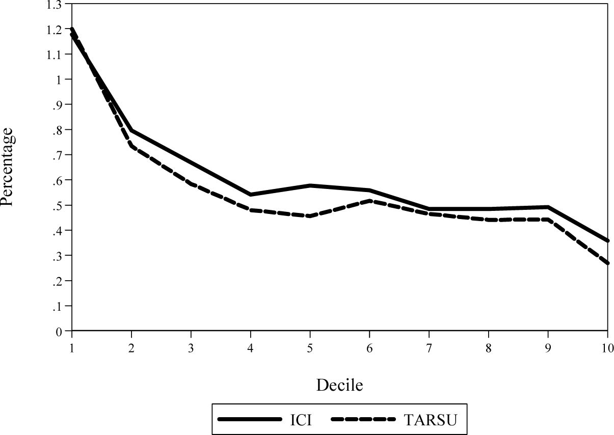
Incidence of ICI and TARSU on main residences.
Figure 1 reports the incidence on gross income of ici and TARSu on main residences by deciles of gross income; only households with positive ICI and TARSU are considered. Both taxes show a similar and moderately regressive impact: both ICI and TARSU are 1.2 percent for the first decile; ICI is 0.4 percent for the top one, while TARSU is 0.3 percent. This is not surprising: a proportional property tax could be progressive with respect to income whenever housing wealth is increasing with respect to income. But ICI do not consider real market values of dwellings, and the cadastral values are highly underestimated. A similar situation is experienced by the TARSU: tax debt is determined by multiplying a tariff per square meter by the total square meters of the dwelling. As long as income increases, the dimension of the dwelling does not increase proportionally.
Figure 2 reports the incidence of House-PIT, ICI and TARSU on dwellings other than the main residence. Only households with at least one dwelling other than the main residence are considered. The incidence of House-PIT is increasing: it is about 0.5 percent for household belonging to the bottom decile and 6 percent for households belonging to the top one. For what it concerns ICI and TARSU, a similar picture with respect to that observed on main residences emerges: ICI paid on other dwellings is 2.1 percent for the bottom decile and 0.8 percent for the top one; the corresponding values for TARSU are 1.3 and 0.3, respectively.
To better characterize the tax progressivity of the system and the role of housing taxation, we consider the Kakwani index, which is defined as the difference between the concentration coefficient for taxes and the Gini coefficient for the gross income (Lambert, 2001). As for taxes, we consider the overall tax system and then we focus on each specific tax on housing considered in the paper. Table 10 reports Kakwani indices for the overall tax-benefit system, the House-PIT, ICI and TARSU. Differently from Figure 1 and 2, here we consider all households. The overall Kakwani index is 0.053. Both ICI and TARSU do not influence tax progressivity, while the House-PIT (which refers to the taxation of second homes, being the main residences exempt) explains about 10% of the overall tax progressivity. This is not surprising given the high percentage of households with their wealth invested in real estates. Given this situation, the Italian policy maker should consider housing taxation and the reform of figurative rents as an important issue for enhancing tax progressivity of the system as a whole. However, this is not what happened in Italy during the last years, as we show in the next section taking as an example the 2008 Property Tax reform.
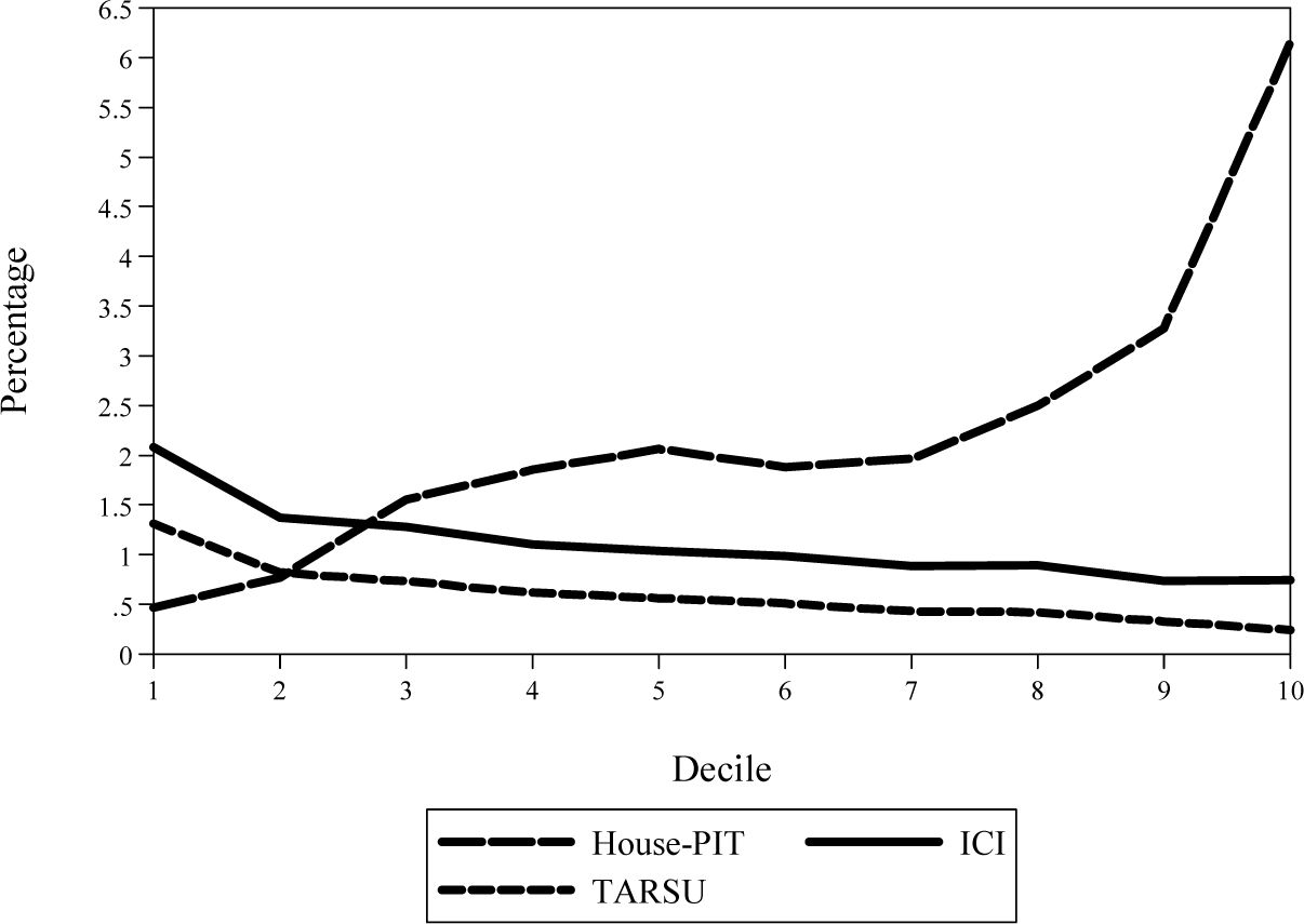
Incidence of House-PIT, ICI and TARSU on dwellings other than the main residence.
Kakwani index.
| Tax | Kakwani index |
|---|---|
| Overall tax-benefit system | 0.05261 |
| House-PIT | 0.00515 |
| ICI | 0.00002 |
| TARSU | -0.00090 |
-
Source: Own calculations based on SHIW-BI.
5. An application: The distributive impact of the 2008 housing taxation reform
Besides studying the distribution of housing taxes in the current system, the microsimulation model developed in the paper is important to simulate the impact of a fiscal policy reform. Here we take as an example the 2008 reform of the Property Tax, that basically exempted the main residence. In principle, given the mild regressivity and the generosity of the current system, one would have expected to observe a reform aimed at reconciling cadastral incomes with current market values. Despite this, no reforms to introduce a sort of mark-to-market mechanisms for the update of cadastral income have been proposed in the last decades. On the contrary, given the high number of owner-occupiers, in order to gain political benefits, from 2008 ownership of the main residence is even exempted from taxation not only with respect to income taxation, but also with respect to the Property Tax. There are two main concerns about this reform: on the one hand, ICI is the most important local tax, so that revenues accruing to Municipalities decreased from about 12 billion euro in 2006 to about 9 billion euro in 2008 (from 5.2 billion euro to 2.4 when considering only dwelling own by households), with the difference being covered by state transfers that limit the local government responsibility; on the other hand, as long as the ownership of the main residence increases the taxpayer ability to pay, the 2008 tax cuts go in the direction of lowering the progressive impact of the tax system as a whole.
Table 11 shows the percentage of households with positive Property Tax both before and after the 2008 reform. In 2006, 16 percent of households with a positive ICI tax base (11.6 percent of all households) had to pay no ICI, since their tax credits were bigger than the gross ICI. Notice that even if tax credits were not linked to household income but to dwelling utilization, most of households actually exempted from the Property Tax were belonging to the left tail of income distribution.
Before the reform about two third of households had a positive ICI. More precisely, about 60% of households had to pay the ICI on the main residence, whilst 30.6% paid ICI on other dwellings. As expected, the percentage of households is moderately increasing with gross income when main residences are considered (values range from 43 to 83.9%); they increase sharply when households owning second homes are considered (values range from 18.8 to 55.5%).
After the 2008 reform, no owner occupier has to pay ICI on the main residence; the actual distribution of the tax is then the one observed on dwellings other than the main residence. Table 11 also shows the tax cuts distribution caused by the reform, which is clearly increasing with income deciles, and mostly concentrated in the top three deciles of the distribution: the top decile benefits one fourth of the overall tax cuts, while the share is 15 percent on the ninth and 11.7 on the eighth; on the other hand, the first decile gains only 4.7 percent, the second 4.8 percent and the third 5.3. The average reduction of tax debt is low: on average, it is about 200 euro, ranging from 142 on the bottom decile to 368 euro on the top one.
To conclude, since the 1980s Italian taxpayers have shown a high sensibility with regard to housing taxation. This explains why both right and left parties have proposed tax cuts on the main residences, and still favor housing with respect to investment in alternative assets. Not surprisingly, political benefits from this reform have been consistent, even though taxpayers’ economic benefits have been very low in absolute value. A tax cut for everyone has no losers, but the distribution of benefits resulted in a more unequal distribution.
Tax cuts distribution of the 2008 housing taxation reform.
| Households with positive ICI (%) | |||||||
|---|---|---|---|---|---|---|---|
| 2006 | 2008 | ||||||
| Decile | Main residence | Other dwellings | Total | Main residence | Other dwellings | Total | Distribution of the tax cuts between 2006 and 2008 |
| 1 | 43.0 | 18.8 | 49.4 | 0.0 | 18.8 | 18.8 | 4.7 |
| 2 | 44.2 | 22.3 | 53.8 | 0.0 | 22.3 | 22.3 | 4.8 |
| 3 | 48.6 | 24.7 | 57.0 | 0.0 | 24.7 | 24.7 | 5.3 |
| 4 | 52.1 | 24.7 | 59.0 | 0.0 | 24.7 | 24.7 | 6.3 |
| 5 | 57.9 | 25.6 | 63.2 | 0.0 | 25.6 | 25.6 | 8.6 |
| 6 | 64.0 | 32.1 | 72.1 | 0.0 | 32.1 | 32.1 | 8.9 |
| 7 | 65.6 | 26.1 | 70.9 | 0.0 | 26.1 | 26.1 | 9.5 |
| 8 | 69.3 | 33.9 | 73.8 | 0.0 | 33.9 | 33.9 | 11.7 |
| 9 | 74.2 | 44.0 | 80.5 | 0.0 | 44.0 | 44.0 | 15.0 |
| 10 | 83.9 | 55.5 | 89.6 | 0.0 | 55.5 | 55.5 | 25.0 |
| Total | 59.9 | 30.6 | 66.6 | 0.0 | 30.6 | 30.6 | 100.0 |
-
Source: Own calculations based on SHIW-BI.
6. Concluding remarks
In this paper we develop a first (static) microsimulation model to study the distributive impact of housing taxation and fiscal policy reforms on Italian households. Our simulations suggest that both Property Tax and Waste Management Tax show a moderate regressive impact with respect to household gross income, whilst the Personal Income Tax on dwellings other than the main residence is progressive. In order to provide an application of our model, we then study the Property Tax reform in 2008, which basically exempted the main residence. All households owning the main residence gain from the 2008 reform, but tax cuts are mostly concentrated on the last three deciles of household equivalent gross income, so that the richest benefited most.
The availability of a microsimulation model specifically devoted to study housing taxation can of course help in a number of directions. One first example is its use for the simulation of alternative policy reforms. For instance, an important question to be asked is relative to the impact of a policy aimed at reconciling cadastral values with market values. The enlargement of the tax base will allow the government to reduce tax wedges on capital and, more importantly, labour incomes. What are the expected effects on efficiency and those on equity is a question that deserves an answer, especially for a country – like Italy – where the reduction of the cost of labour is a highly debated issue. A second example is related to political economy issues: the microsimulation model will allow us to define net gainers and net losers when implementing a policy reform, hence explaining whether or not a given policy has any chances to be really implemented in terms of political support.
Needless to say, the model can be further improved, in particular incorporating behavioural responses. As it is well known, a static model does not incorporate by definition individuals’ reactions to a change in tax policy parameters. For instance, we cannot answer to questions such as what happens to current market prices in the housing market when we include in the PIT tax base current market values. This is left for future research.
Footnotes
1.
The life-tenant retains the right (which is legally labelled ‘usufruct’) to freely use the dwelling for all her life. The owner then has just the ‘bare property’ of the building, but no rights to use it.
2.
The value of the dwelling is then equal to the perpetual annuity of the cadastral income with a 1 percent discount rate.
3.
See Brandolini (1999) and Bank of Italy (2008) for details.
4.
Almost all the owner-occupiers (88.7 percent) are not burdened with a mortgage, while only a small percentage (11.3 percent) have a mortgage.
5.
As for tenants, almost 70 percent rent the house from other households; 25.7 percent of tenants rent from public bodies, like the Istituto Autonomo Case Popolari (a locally funded Institute providing housing to the poor), but also – to a minor extent – Regions, Provinces, Municipalities; and 4 percent from private firms.
6.
We consider here children all individuals within the household aged 17 or less.
7.
Different equivalence scales have been proposed. The Cutler and Kats scale is the most general, since most of the other equivalence scales can be obtained by varying its parameters. It can be also useful in sensitivity analysis. More precisely, according to van de Ven and Creedy (2005) methodology, a close approximation of the government implicit scale can be obtained by choosing scale parameters that minimise the re-ranking.
References
- 1
- 2
-
3
Household Income and Wealth in 2006Bank of Italy, Supplements to the Statistical Bulletin 7, XVIII.
-
4
The Distribution of Personal Income in Post-War Italy: Source Description, Data Quality, and the Time Pattern of Income Inequality. Working paper 350Bank of Italy.
-
5
Modello di Microsimulazione EconLav: la costruzione del data-set di input. Working papers 4Modello di Microsimulazione EconLav: la costruzione del data-set di input. Working papers 4, Ministry of Economy and Finance, Department of Finance.
- 6
-
7
Home ownership and the Welfare State: is Southern Europe different?South European Politics and Society 1:163–185.
-
8
Imputation of gross amounts from net incomes in households surveys. An application using EUROMOD. Working paper EM1EUROMOD.
-
9
The distribution and redistribution of incomeManchester: Manchester University Press.
-
10
The impact of mortgage interest tax relief in the Netherlands, Sweden, Finland, Italy and Greece. Working paper EM2EUROMOD.
- 11
-
12
L’ICI: una valutazione a un decennio dalla sua introduzioneEconomia Pubblica 5–6:143–170.
- 13
Article and author information
Author details
Acknowledgements
We wish to thank the editors Gijs Dekkers and Eveline van Leeuwen, an anonymous referee, Massimo Baldini and seminar participants at the 2nd General Conference of the International Microsimulation Association “Microsimulation: Bridging Data and Policy", Ottawa, June 8–10, 2009, for helpful comments on previous drafts of this paper. Usual disclaimers apply.
Publication history
- Version of Record published: August 31, 2011 (version 1)
Copyright
© 2011, Pellegrino et al.
This article is distributed under the terms of the Creative Commons Attribution License, which permits unrestricted use and redistribution provided that the original author and source are credited.