A mate-matching algorithm for continuous-time microsimulation models
- Max Planck Institute for Demographic Research, Germany
Cite this article
as: S. Zinn; 2012; A mate-matching algorithm for continuous-time microsimulation models; International Journal of Microsimulation; 5(1); 31-51.
doi: 10.34196/ijm.00066
- Article
- Figures and data
- Jump to
Figures
Figure 1

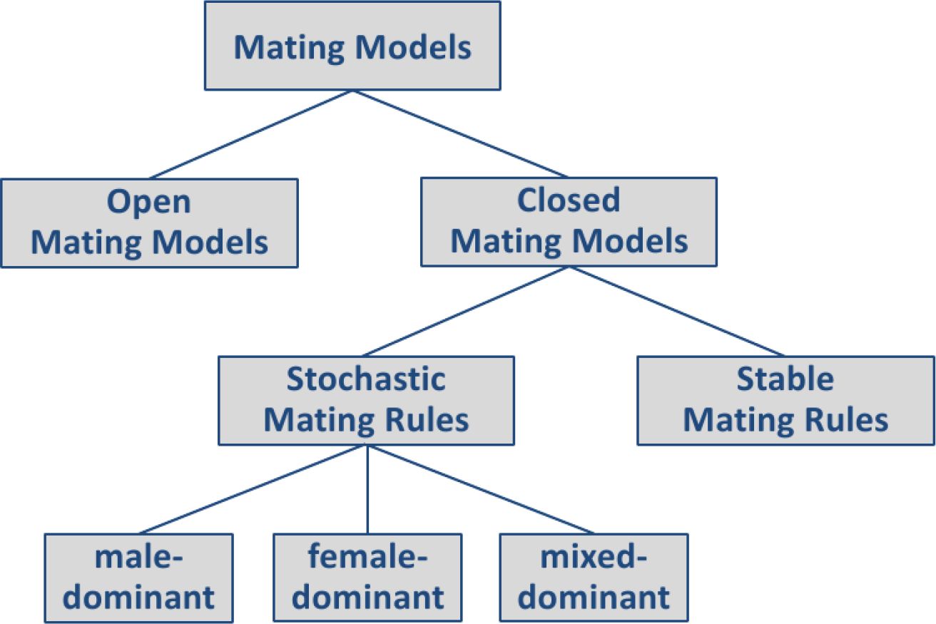
Classification of mating models and mate-matching algorithms for microsimulation.
Figure 2

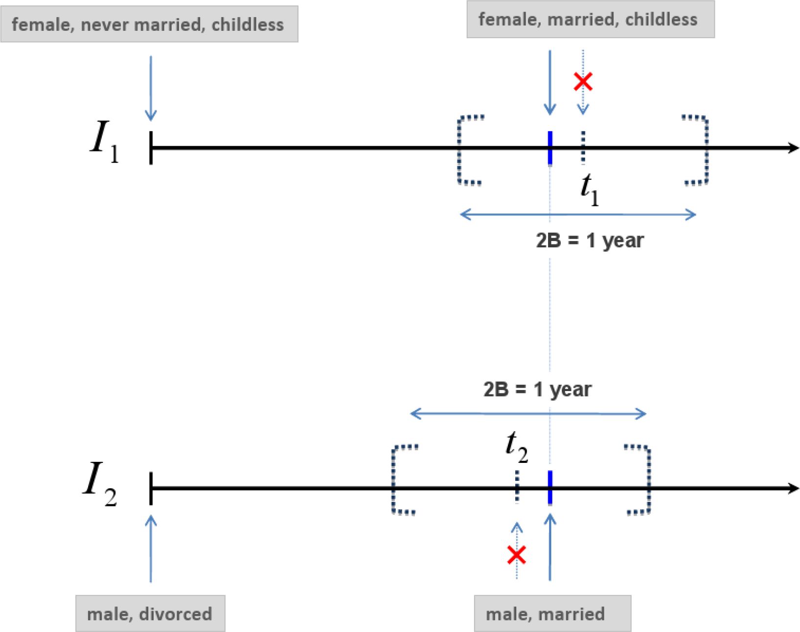
Woman I1 experiences a marriage event at time t1. Man I2 experiences a marriage event at time t2. As t1 ∈ [t2 − 0.5 years, t2 + 0.5 years] and t2 ∈ [t1 − 0.5 years, t1 + 0.5 years] both individuals have overlapping searching periods and might meet during the mating process.
Hence, they can be considered as potential spouses. Their formation time would be if they were actually linked in the mate-matching algorithm.
Figure 3
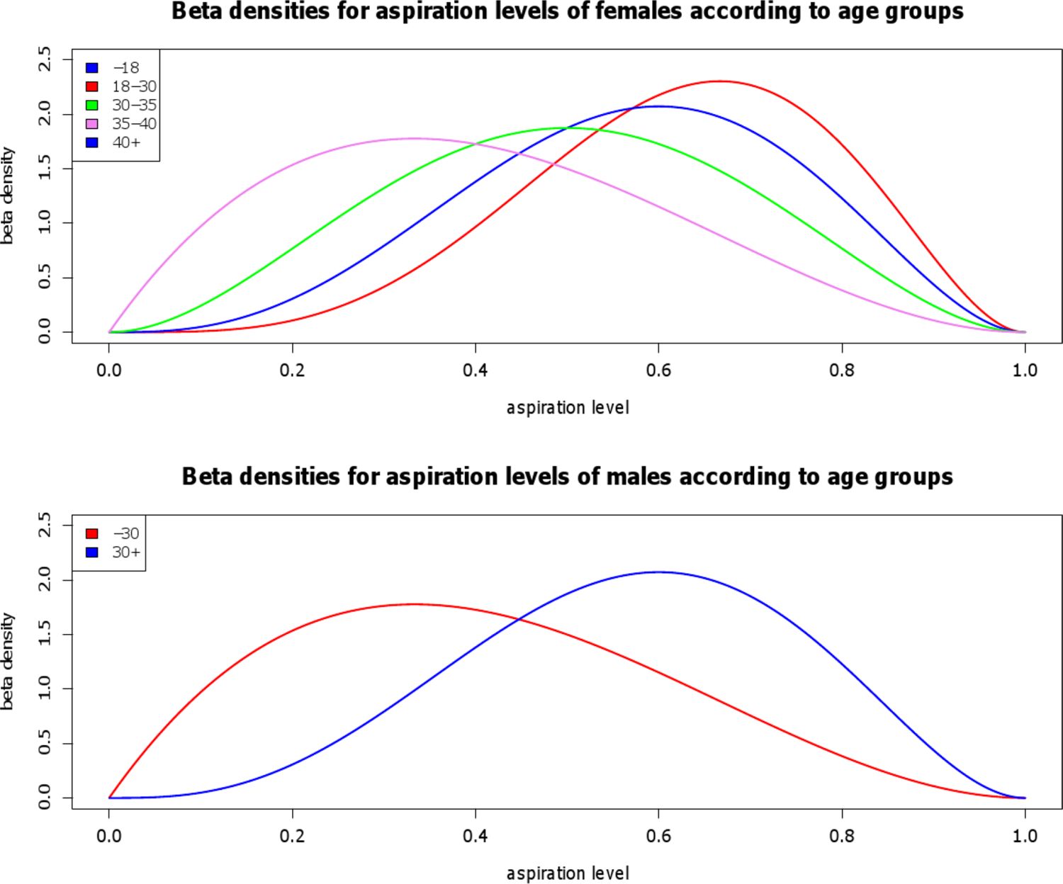
Densities of the beta distributions that are used to determine aspiration levels regarding partners. The densities vary with gender and age. For females, four different curves are applied: one below age 18, one for ages between 18 and 30, one between ages 30 and 35, and one after age 40. For males, two different curves are applied: one for males younger than 30 and the other after age 30.
Figure 4

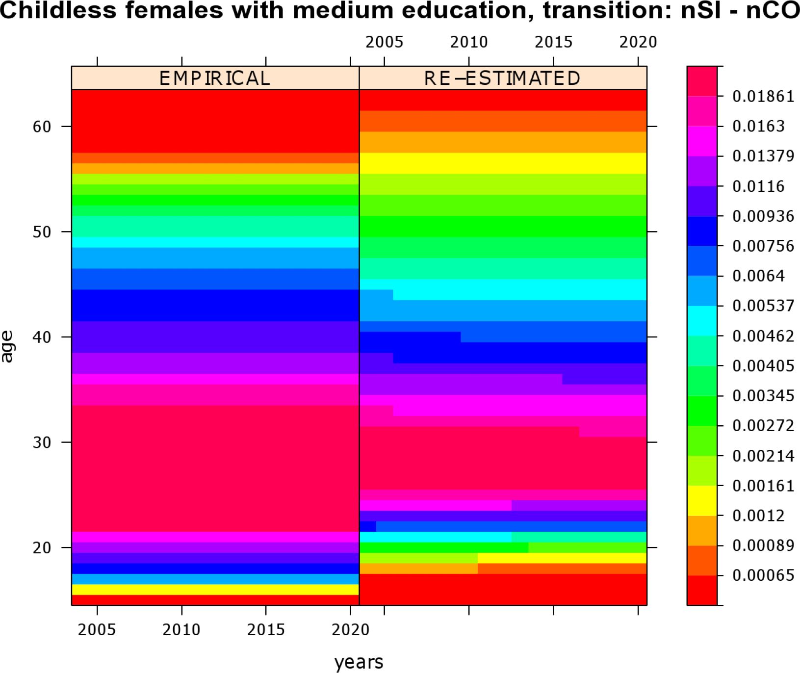
Re-estimation of transition rates of childless females with a lower secondary (medium) education who experience a transition from “being single after leaving parental home” (nSl) to “first cohabitation” (nCO).
Figure 5

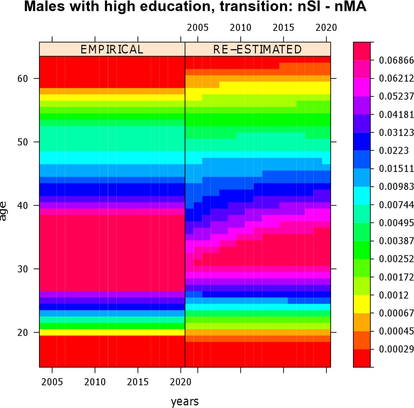
Re-estimation of transition rates of highly educated males who experience a transition from “being single after leaving parental home” (nSI) to “married” (nMA).
Figure 6

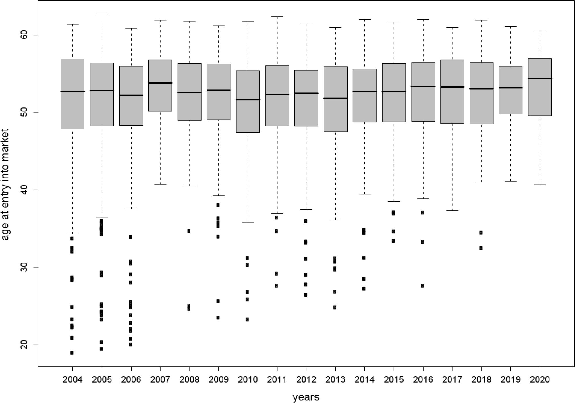
Age distribution of unsuccessful seekers at the time when they enter the partnership market.
Figure 7

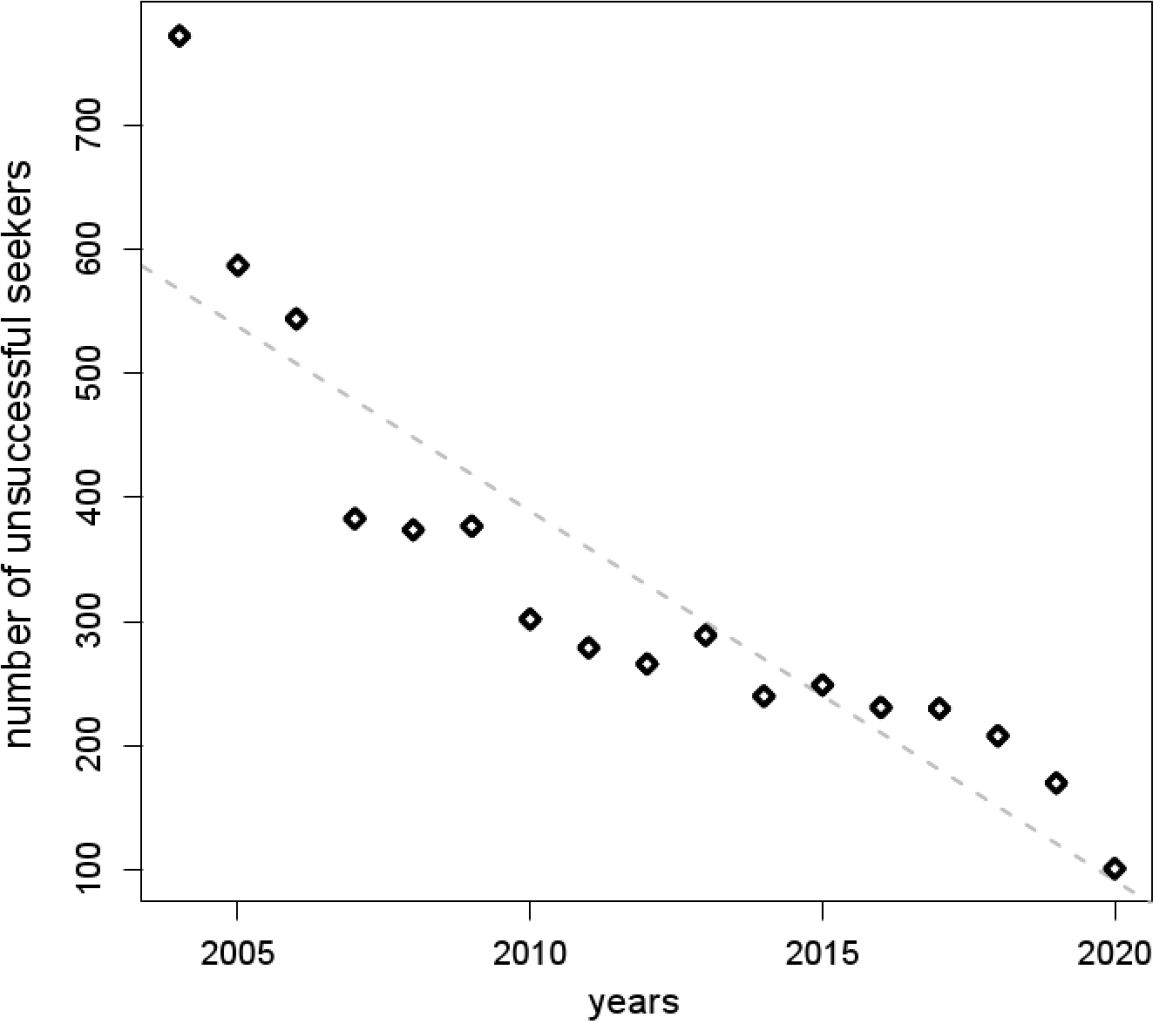
Number of unsuccessful seekers according to the year when they initialize a partner search.
Figure 8

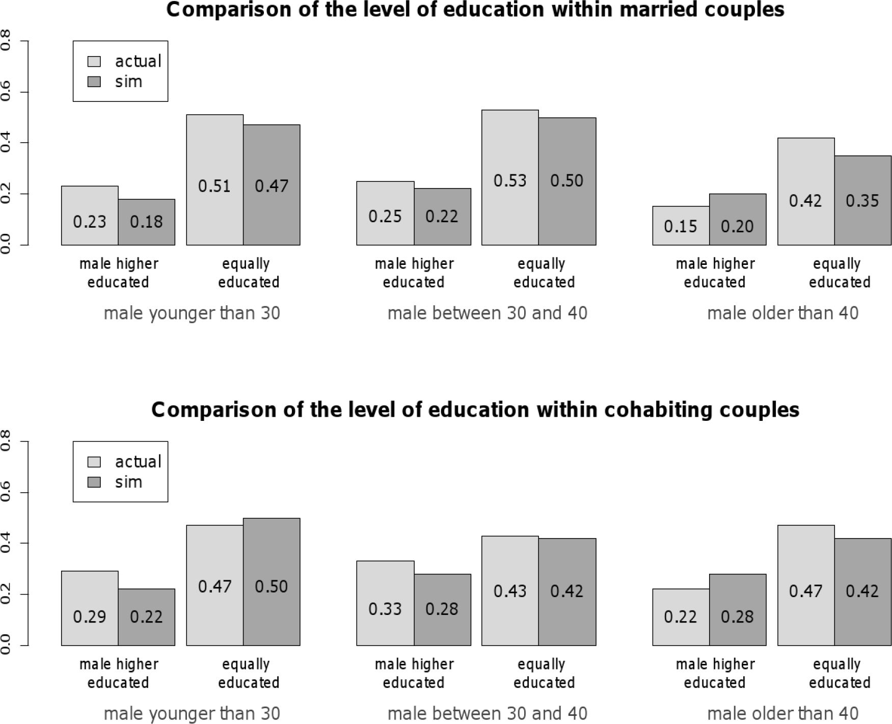
Differences in the educational level of spouses in observed and simulated couples. Each bar shows the percentage of females in the corresponding category.
Figure 9
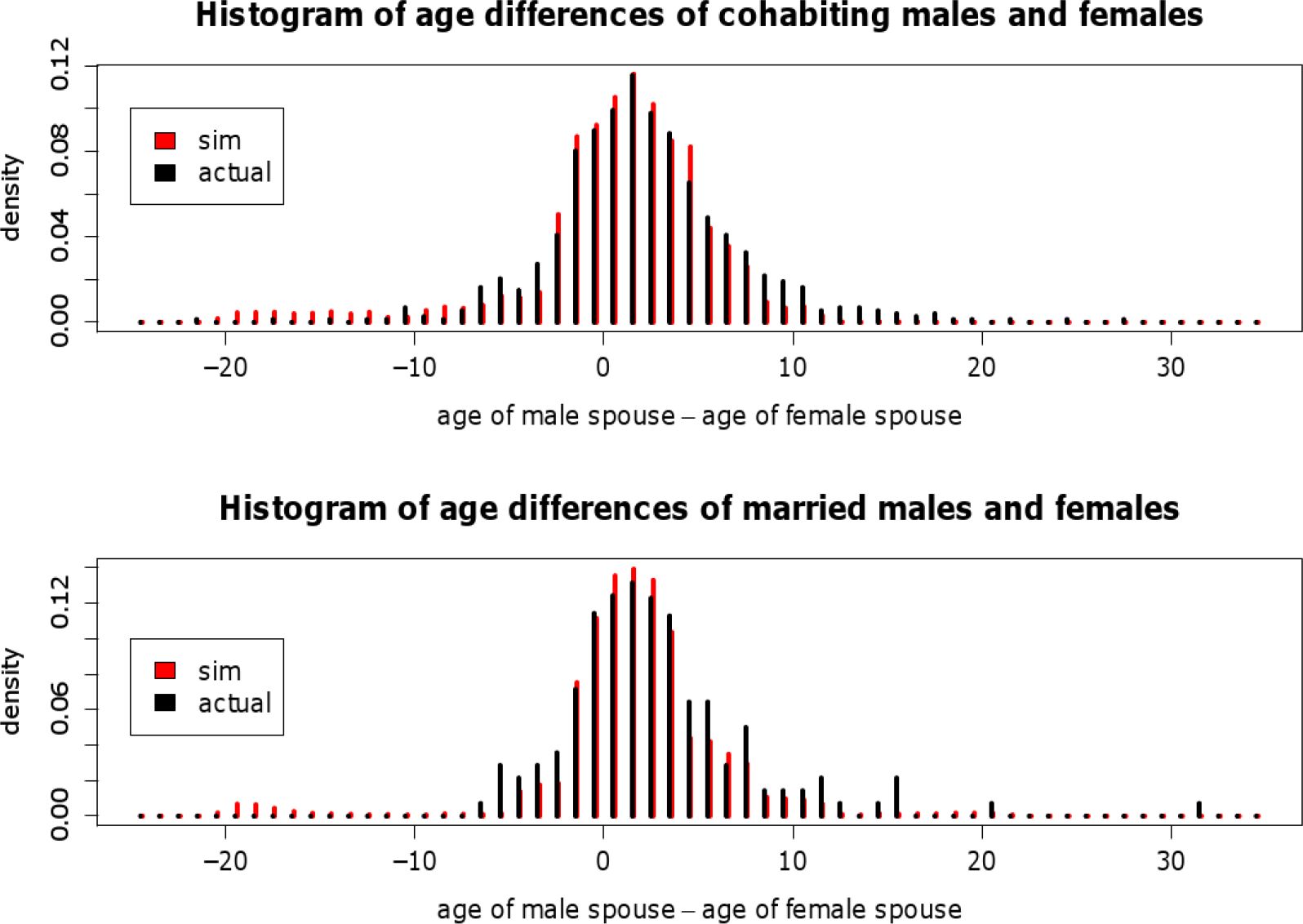
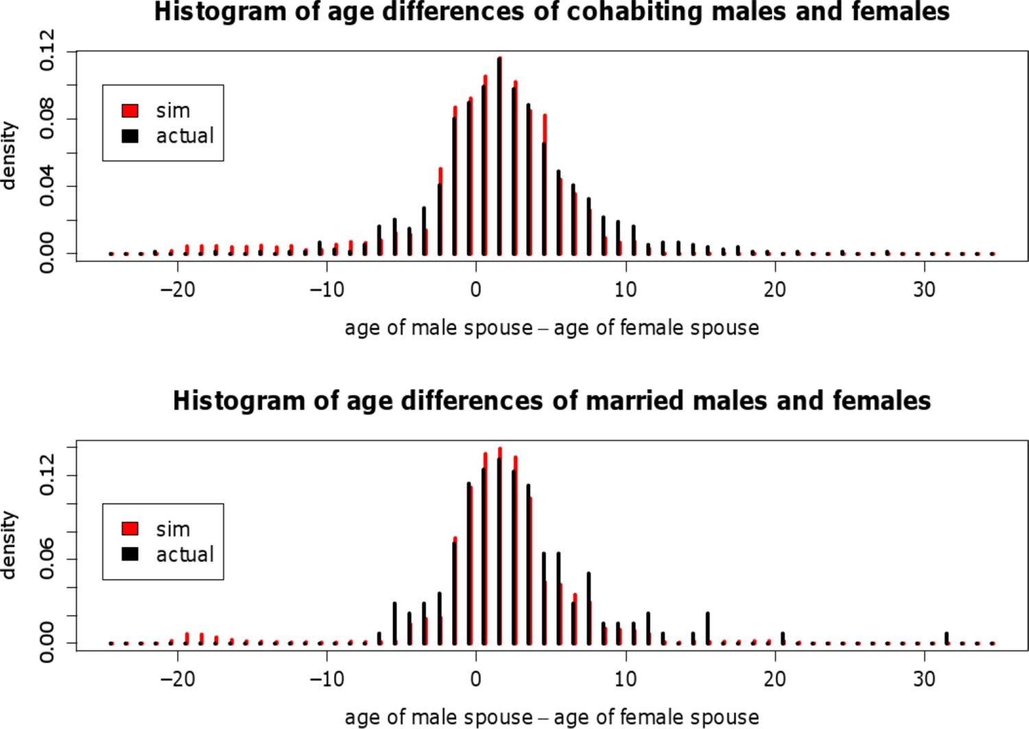
Age differences of spouses in observed and simulated couples.
Figure 10
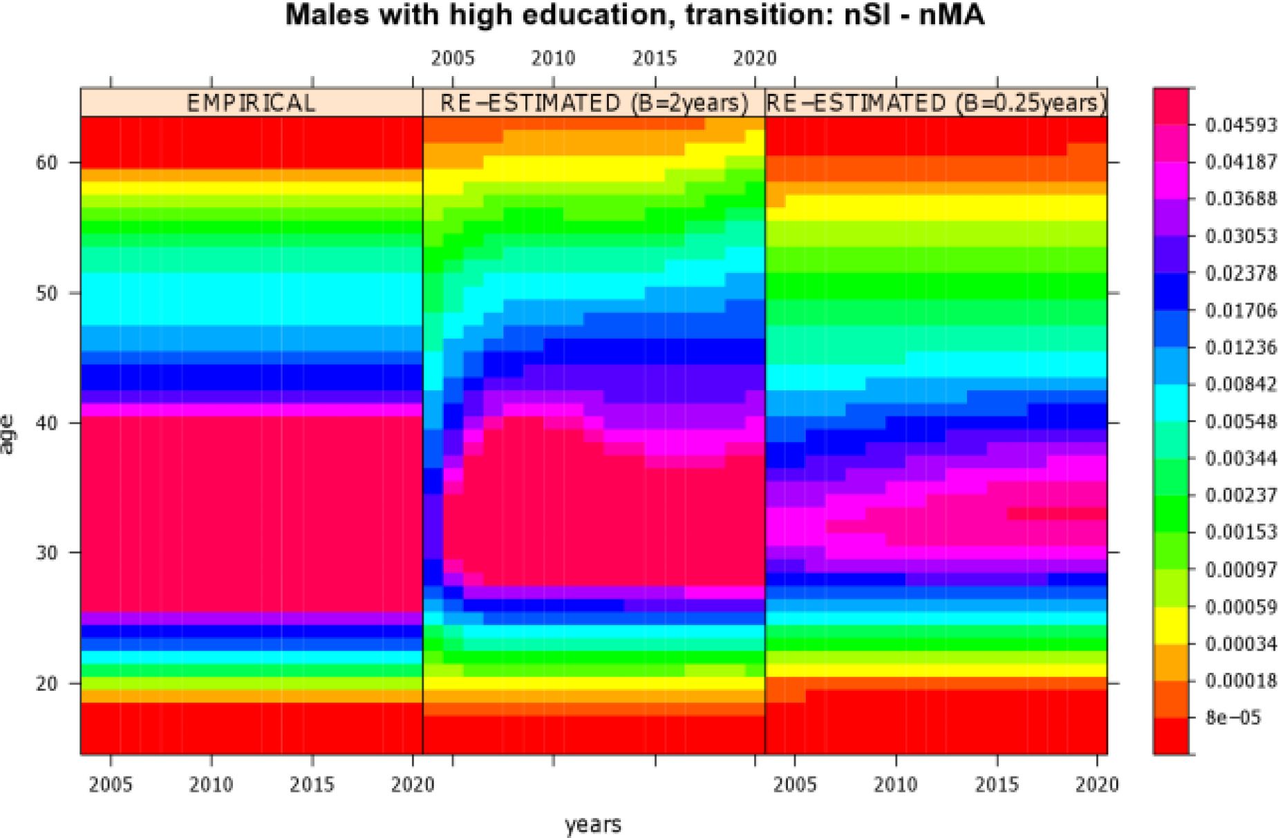

Comparison of re-estimated transition rates of highly educated males who experience a transition from “being single after leaving parental home” (nSI) to “married” (nMA). The left graph shows the empirical input rates used. The graph in the middle displays re-estimated rates from a simulation run with B = 2 years (intersection of the searching periods), and the right graph shows re-estimated rates from a simulation run with B = 0.25 years.
Tables
Table 1
Parameters and suggested parameter values for the present stochastic mate-matching procedure.
| Description | Parameter | Value |
|---|---|---|
| Intersection of searching periods | B | 0.5 |
| Upper bound of number of potential spouses | N | normally distributed, μ = 120, σ = 30 |
| Individual aspiration level | ai | beta distributed, gender- & age-dependent (cp. Figure 3) |
| Decrement of aspiration level in case of rejection | δA | 0.1 |
| Bound for small pool size | sp | 10 |
| Decrement of aspiration level in case of small pool size | δB | 0.3 |
Table 2
Regression results of Model 1 (entering first cohabitation) and 2 (entering higher order cohabitation).
| Model 1 | ||
|---|---|---|
| Variable | Coefficient | p-value |
| Age of male | 0.0521 | 0.0046 |
| Age difference (age of male – age of female) | ||
| greater than 9 | −2.9876 | <0.001 |
| from 7 to 9 | −1.4633 | <0.001 |
| from 4 to 6 | −0.4862 | 0.0108 |
| from −3 to 3 | 0 | |
| from −6 to −4 | −1.4360 | <0.001 |
| from −10 to −7 | −2.8137 | <0.001 |
| smaller than −10 | −3.0582 | <0.001 |
| Difference in educational level | ||
| male is higher or equally educated | 0.6424 | <0.001 |
| Marriage history of female | ||
| female was married before | -0.2811 | 0.1833 |
| Number of potential pairs: 1078 | ||
| Model 2 | ||
|---|---|---|
| Variable | Coefficient | p-value |
| Age of male | 0.0550 | 0.0013 |
| Age difference (age of male – age of female) | ||
| greater than 10 | −3.5428 | <0.001 |
| from 4 to 10 | −3.5428 | <0.001 |
| from −3 to 3 | 0 | |
| from −10 to −4 | −1.0105 | 0.0021 |
| smaller than −10 | −3.1277 | 0.0196 |
| Difference in educational level | ||
| male is higher or equally educated | 0.7825 | 0.0148 |
| Children with former partner | ||
| female has children | 1.6754 | <0.001 |
| Number of potential pairs: 394 | ||
Table 3
Regression results of Model 3 (entering first marriage) and 4 (entering higher order marriage).
| Model 3 | ||||
|---|---|---|---|---|
| Variable | Coefficient | p-value | ||
| Age of male | 0.0646 | 0.0650 | ||
| Age difference (age of male – age of female) | ||||
| greater than 10 | −3.3997 | < 0.001 | ||
| from 7 to 10 | −1.4934 | 0.0110 | ||
| from 3 to 6 | −0.8026 | 0.0692 | ||
| from −2 to 2 | 0 | |||
| from −5 to −3 | −1.5026 | 0.0263 | ||
| smaller than −5 | −4.3357 | < 0.001 | ||
| Difference in educational level | ||||
| male is higher or equally educated | 0.8493 | 0.0525 | ||
| Marriage history of female | ||||
| female was married before | −0.4314 | 0.4873 | ||
| Number of potential pairs: 198 | ||||
| Model 4 | ||
|---|---|---|
| Variable | Coefficient | p-value |
| Age of male | −0.0120 | 0.6618 |
| Age difference (age of male – age of female) | ||
| greater than 8 | −2.9174 | < 0.001 |
| from 4 to 8 | −1.6287 | 0.0547 |
| from −3 to 3 | 0 | |
| smaller than −4 | −3.2270 | < 0.001 |
| Difference in educational level | ||
| male is higher or equally educated | 1.2949 | 0.0743 |
| Number of potential pairs: 82 | ||
Download links
A two-part list of links to download the article, or parts of the article, in various formats.