Figures and data in Modelling private wealth accumulation and spend-down in the Italian microsimulation model CAPP_DYN: A life-cycle approach

Cite this article as: S. Tedeschi, E. Pisano, C. Mazzaferro, M. Morciano; 2013; Modelling private wealth accumulation and spend-down in the Italian microsimulation model CAPP_DYN: A life-cycle approach; International Journal of Microsimulation; 6(2); 76-122. doi: 10.34196/ijm.00084

10 figures and 8 tables

Figures

Figure 1

Download asset Open asset

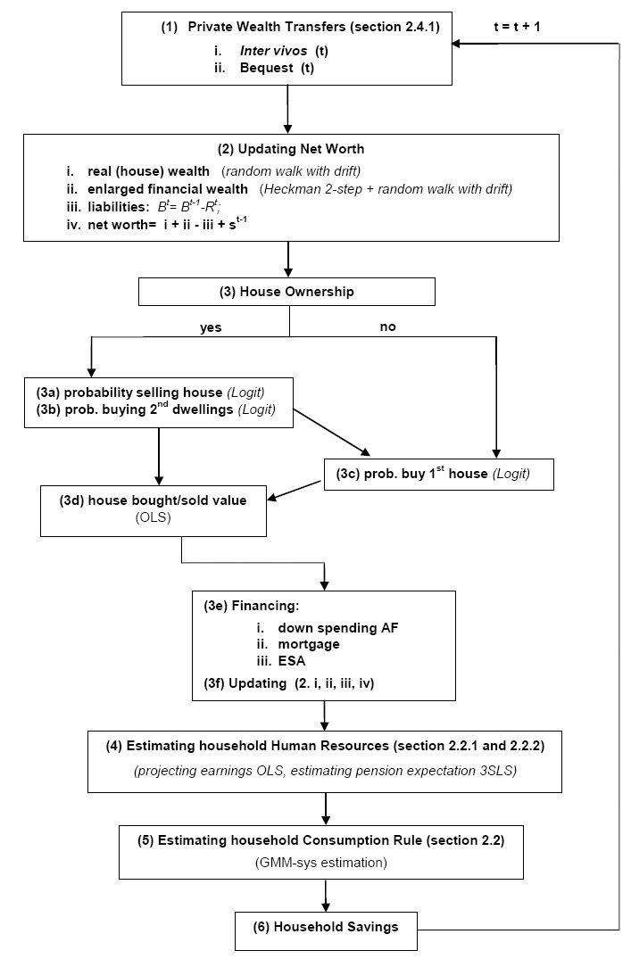
A stylized scheme of formation and transmission of wealth in the wealth module.

Figure 2

Download asset Open asset

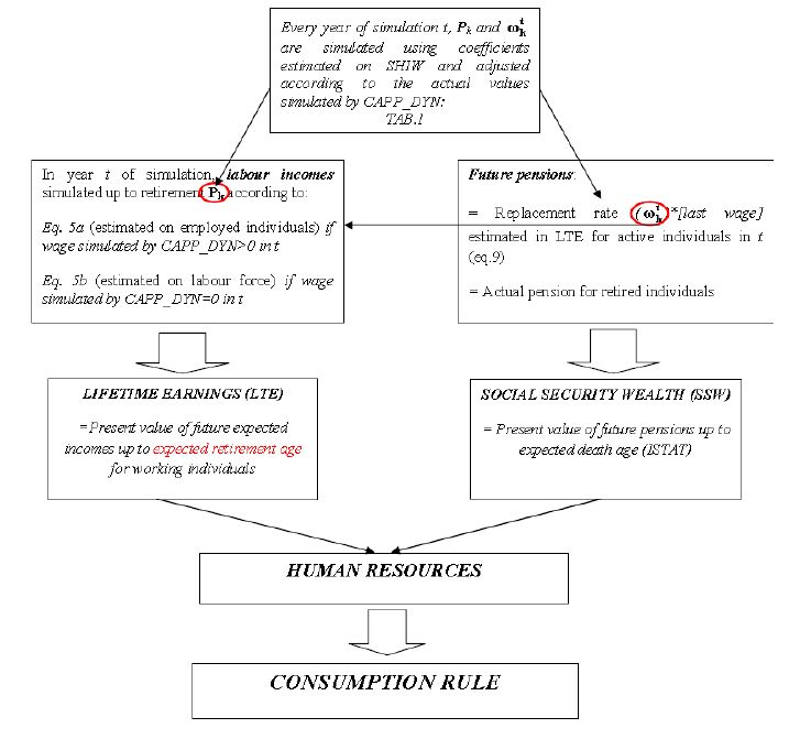
Estimation and simulation of human resources.

Figure 3

Download asset Open asset

Average equivalent consumption (left) and propensity to save (right) household-head-age-profile.

Figure 4

Download asset Open asset

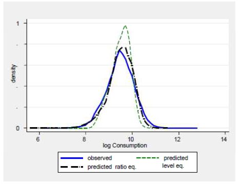
Post-estimation predicted consumption from dynamic model in level vs ratio.

Figure 5

Download asset Open asset

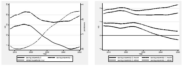
Average saving propensity (left), propensity to save for active households vs. for retired households (right), 2008–2050.

Figure 6

Download asset Open asset

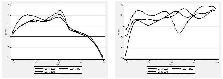
Propensity to save by age, LC (left) vs. NS (right) simulation, 2011–2020, 2021–2030, 2036–2045 (averages).

*Source*: Authors’ computations on simulation results.

Figure 7

Download asset Open asset

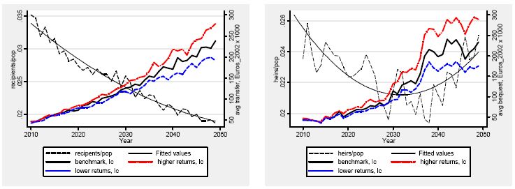
Evolution of iv and mc transfers recipient households’ share and of the average amount received, 2010–2050.

*Source*: Authors’ computations on simulation results (2008–2050).

Figure 8

Download asset Open asset

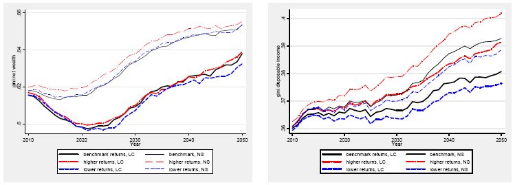
Evolution in the Gini of net worth (left) and disposable income (right), 2010–2050.

*Source*: Authors’ elaboration on simulation results.

Figure 9

Download asset Open asset

Contributions to wealth Gini variation, LC (left) vs. NS (right) simulation, 2008–2050.

Figure 10

Download asset Open asset

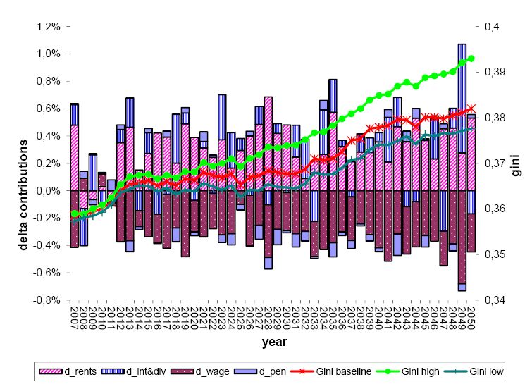
Differential contributions to disposable income Gini variation between high and low returns scenarios, 2007–2050.

*Source*: Authors’ computations on simulated data.

Tables

Table 1

Three-stage least-squares regression of planned age of retirement and the expected replacement rate.

Equation	Obs	Parms	RMSE	R-sq	chi2	P
1. PRA	27194	21	3.435451	0.257	9408.45	0
2. ERR	27194	21	0.163388	0.149	5043.9	0
Planned Age of Retirement				Expected Replacement Rate
	B		SE		B		Se
year_contrib	−0.5187 ***		0.0138	PRA	0.0026 **			0.0010
year_contrib²	−0.0093 ***		0.0003	year_contrib	0.0064 ***		0.0009
age*contrib.	0.0148 ***		0.0003	age*contrib	0.0000		0.0000
female	−2.0137 ***		0.0523	NDC	−0.0292		0.0180
NDC	0.1496		0.3824	single	−0.0024		0.0050
Education (omit.lower secondary)
upper_secondary	0.2877 ***		0.0557	upper secondary	0.0130 ***		0.0026
degree_or_more	0.8929 ***		0.0842	degree or more	0.0094 *		0.0040
self_employed	1.2709 ***		0.0646	self employed	−0.1168 ***		0.0033
public	−0.2373 ***		0.0632	public	0.0457 ***		0.0030
home_owner	−0.1369 *		0.0564	partime	−0.0363 ***		0.0047
South	0.6384 ***		0.0580	Centre	0.0321 ***		0.0030
single	0.3774 ***		0.1072	South	0.0427 ***		0.0030
tau2002	0.0625		0.0751	tau2002	−0.0298 ***		0.0035
tau2004	0.2979 ***		0.0774	tau2004	−0.0453 ***		0.0036
tau2006	0.0922		0.0805	tau2006	−0.0739 ***		0.0037
tau2008	0.8402 ***		0.0978	tau2008	−0.0793 ***		0.0047
Cohort effect (omit. Cohorts <1953)
coor_53	1.1369 ***		0.1010	coor_53	0.0122 **		0.0046
coor_58	2.0562 ***		0.1234	coor_58	0.0165 **		0.0056
coor_63	2.5093 ***		0.1462	coor_63	0.0257 ***		0.0065
coor_68	2.5112 ***		0.1672	coor_68	0.0393 ***		0.0071
coor-73	2.3387 ***		0.1844	coor-73	0.0660 ***		0.0075
coor_78	2.0769 ***		0.2041	coor_78	0.0688 ***		0.0081
intercept	61.3483 ***		0.1937	intercept	0.4269 ***		0.0635
Endogenous variables: PRA, ERR

*

p<.05.
**

p<.01.
***

p<.001.
Source: Authors’ computations on SHIW 2000–2008.

Table 2

Dynamic panel-data estimation of the consumption rule, two-step system GMM ¹⁶.

ln{C/HR}	B	Se
Lag.ln{C/HR}	0.0821 ***	0.0209
In_af_en	0.0114 ***	0.0024
In_ar_h	−0.0171 ***	0.0014
In_ar_h*n_houses	0.0040 ***	0.0006
In_pf	0.0092 ***	0.0012
quintile 2_income	−0.1347 ***	0.0181
quintile 3_income	−0.1832 ***	0.0206
quintile 4_income	−0.2559 ***	0.0232
quintile 5_income	−0.3105 ***	0.0272
hh_age	−0.2152 ***	0.0491
hh_age²	0.0066 ***	0.0013
hh_age³	−0.0001 ***	0.0000
hh_age⁴	0.0000 ***	0.0000
hh_age_self_emp	−0.0026 ***	0.0004
hh_age_upper_secondary	−0.0009 ***	0.0002
hh_age_degree_or_more	−0.0032 ***	0.0004
h_res_life	−0.0143 ***	0.0027
hh_retired	−0.1282 ***	0.0213
earners_ratio	−0.2058 ***	0.0326
n_child_in the family	0.0232 **	0.0087
South	−0.0489 ***	0.0109
Household types (omitt. Nuclear family)
Single	0.0108	0.0211
nuclear single headed	0.1754 ***	0.0356
non_nuclear single headed	0.4704 ***	0.0350
non_nuclear	0.1948 ***	0.0174
Time dummies (omit.tau2002)
tau1993	0.0148	0.0191
tau1995	0.0623 **	0.0193
tau1998	−0.0699 ***	0.0210
tau2000	−0.4194 ***	0.0194
tau2004	−0.0219	0.0176
tau2006	0.0228	0.0186
tau2008	0.0018	0.0182
intercept	−0.2847	0.6923

N = 23,426, number of groups = 10,284.
Arellano-Bond test for AR(1) in first differences: z = −18.00 Pr > z = 0.000.
Arellano-Bond test for AR(2) in first differences: z = 0.49 Pr > z = 0.627.
Sargan test of overid. restrictions: chi2(7) = 7.60 Prob > chi2 = 0.369.
Hansen test of overid. restrictions: chi2(7) = 4.79 Prob > chi2 = 0.685.
Difference-in-Hansen tests of exogeneity of instrument subsets:
GMM instruments for levels.
Hansen test excluding group: chi2(6) = 4.60 Prob > chi2 = 0.596.
Difference (null H = exogenous): chi2(1) = 0.20 Prob > chi2 = 0.658.
*

p<.05.
**

p<.01.
***

p<.001.
Source: Authors’ computations on SHIW data, Historical Archive, panel component, waves 1991–2008.

Table 3

Two-step estimation for intergenerational giving with Heckman correction.

Donor side N=16,871
Logit Probability of being Donor			OLS ln{Ratio}
	B	Se		B	Se
age	0.0807 ***	0.0243	age	−0.7785 **	0.2404
age²	−0.0007 ***	0.0002	age²	0.0113 **	0.0036
in_work	0.3522 ***	0.052	age3	−0.0001 **	0.000
quintile 3_wealth	0.4146 ***	0.0543	in work	−0.4384 ***	0.0866
quintile 4_wealth	0.6046 ***	0.0531	retired	−0.2449 **	0.0849
quintile 5_wealth	0.6989 ***	0.0531	unemp	−0.4619 **	0.1649
child_unemp	0.2835 ***	0.0625	ch_unemp	0.3006 ***	0.0817
wed_or_birth	3.2668 ***	0.1205	quintile 3_wealth	−0.5422 ***	0.0752
upper_secondary	0.5074 ***	0.0463	quintile 4_wealth	−0.8931 ***	0.0736
degree_or_more	0.742 ***	0.0502	quintile 5_wealth	−1.4278 ***	0.0733
Italy	−0.2737 ***	0.0747	Italy	0.7029 ***	0.0951
_intercept	−4.4368 ***	0.8158	mills_ratio	0.2653 ***	0.0414
			_intercept	15.5409 **	5.3305

T
*

p<.05.
**

p<.01.
***

p<.001.
Source: Authors’ computations on SHARE data, wave 2004.

Table 4

Two-step estimation for intergenerational receiving without Heckman correction.

Recipient side
N=29,652 Logit Probability of being Recipient			N= 1,872 OLS ln{Amount}
	B	t		B	Se
In(af parents)	0.169 ***	0.061	In(af parents)	0.0892 ***	0.0079
age	−0.0883 ***	0.052	age	0.0253 *	0.0147
age²	0.0007 ***	0.0543	age²	−0.0004 *	0.0002
married	0.3004 **	0.0531	grandchildren	−0.1051 *	0.0567
single	0.6497 ***	0.0531	married	0.1911 ***	0.0494
divorced	0.6462 ***	0.0625	Italy	0.2481 **	0.0944
in work	−0.2689 ***	0.1205	_intercept	7.028 ***	0.2699
degree	0.3421 ***	0.0463
grandchildren	0.2863 ***	0.0502
Italy	0.1984 **	0.0747
_intercept	−1.3815 ***	0.8158

T
*

p<.05.
**

p<.01.
***

p<.001.
Source: Authors’ computations on SHARE data, wave 2004.

Table 5

Cumulated contributions to wealth Gini variation, LC vs. NS simulation, 2008–2050 (in percent).

	W₀	Capgains	S	ig_tr	ESA	d.gini
1.LC approach	0.146	−3.918	−0.511	6.757	−1.958	0.516
2.NS approach	0.128	−4.522	6.754	2.979	−1.705	3.634
(1)– (2)	−0.018	−0.604	7.264	−3.778	0.253	3.118

Source: Authors’ computations on simulated data.

Table 6

Cumulated contributions to disposable income Gini variation, LC approach, different returns scenarios, 2008–2050 (in percent).

	After_tax pensions	After-tax earnings	Rents on real estate net of liabilities	Interests on financial wealth	d.gini	avg r-g
2.low returns	5.55	−1.42	2.50	3.51	10.13	0.13
1.Benchmark	5.28	−6.69	7.57	4.92	11.08	0.61
3.High returns	4.79	−14.70	16.89	6.89	13.88	1.28
(3)-(2)	−0.76	−13.28	14.40	3.39	3.75	1.15

Source: Authors’ computations on simulated data.

Table 7

Cumulated variation in incomes shares (in percent).

Sources	2008	2050	2050–2008	2008	2050	2050–2008	2008	2050	(2050)-(2008)
After-tax earnings	51.0	43.8	−7.2	51.4	46.2	−5.2	50.7	40.0	−10.7
After-tax pensions	29.7	29.7		29.9	31.3	1.5	29.5	27.2	−2.3
Rents on real estate net of negative interests	14.6	18.3	3.7	14.1	15.1	1.1	15.2	23.7	8.6
Interests on financial wealth	4.7	8.2	3.4	4.7	7.4	2.7	4.7	9.1	4.4

Source: Authors’ computations on simulated data.

Table A1

Table A1 Exogenous parameters (per year).

Low returns scenario	Benchmark returns scenario	High returns scenario
Productivity	Productivity	Productivity
Same as benchmark	G (average earnings growth)	Same as benchmark
“	0.88% (2008–2009)	“
“	1.00% (2010–2013)	“
“	1.20% (2014–2019)	“
“	1.90% (2020–2029)	“
“	2.00% (2030–2050)	“
Capital gains	Capital gains	Capital gains
r_h ~N µ=0.75%; sd=8%	r_h ~N µ= 1.5%; sd= 8%	r_h ~N µ=2.5%; sd=8%
r_f ~N µ=1.5%; sd=18%;	r_f ~N µ=3%; sd=18%;	r_f ~N µ=5%; sd=18%;
kurt = 2.4%	kurt=2.4%	kurt=2.4%
r_esa=0.9%	r_esa=0.9%	r_esa=0.9%
Interests and rents	Interests and rents	Interests and rents
Same as benchmark	r_m ~N µ=3%; sd= 0.5%	Same as benchmark
“	home equity annual rent: 3.5%	“
“	real interest rate on non-risky AF: 1%	“
“	real interest rate on risky AF: 3%	“

Download links

A two-part list of links to download the article, or parts of the article, in various formats.

Downloads (link to download the article as PDF)

Article PDF

Download citations (links to download the citations from this article in formats compatible with various reference manager tools)

BibTeX
RIS

Open citations (links to open the citations from this article in various online reference manager services)

Mendeley

A stylized scheme of formation and transmission of wealth in the wealth module.

Estimation and simulation of human resources.

Average equivalent consumption (left) and propensity to save (right) household-head-age-profile.

Post-estimation predicted consumption from dynamic model in level vs ratio.

Average saving propensity (left), propensity to save for active households vs. for retired households (right), 2008–2050.

Propensity to save by age, LC (left) vs. NS (right) simulation, 2011–2020, 2021–2030, 2036–2045 (averages).

Evolution of iv and mc transfers recipient households’ share and of the average amount received, 2010–2050.

Evolution in the Gini of net worth (left) and disposable income (right), 2010–2050.

Contributions to wealth Gini variation, LC (left) vs. NS (right) simulation, 2008–2050.

Differential contributions to disposable income Gini variation between high and low returns scenarios, 2007–2050.

Three-stage least-squares regression of planned age of retirement and the expected replacement rate.

Dynamic panel-data estimation of the consumption rule, two-step system GMM 16.

Two-step estimation for intergenerational giving with Heckman correction.

Two-step estimation for intergenerational receiving without Heckman correction.

Cumulated contributions to wealth Gini variation, LC vs. NS simulation, 2008–2050 (in percent).

Cumulated contributions to disposable income Gini variation, LC approach, different returns scenarios, 2008–2050 (in percent).

Cumulated variation in incomes shares (in percent).

Table A1 Exogenous parameters (per year).

Downloads (link to download the article as PDF)

Download citations (links to download the citations from this article in formats compatible with various reference manager tools)

Open citations (links to open the citations from this article in various online reference manager services)

Dynamic panel-data estimation of the consumption rule, two-step system GMM ¹⁶.