Data and model cross-validation to improve accuracy of microsimulation results: Estimates for the polish household budget survey
- Centre for Economic Analysis, Poland
Abstract
We conduct detailed analysis of the Polish Household Budget Survey data for the years 2006–2011 with the focus on its representativeness from the point of view of microsimulation analysis. We find important discrepancies between the aggregate data weighted with baseline grossing-up weights and official statistics from other sources. A number of re-weighting exercises is examined from the point of view of the accuracy of microsimulation results. We show that using a combination of variables from the data together with a small number of outcomes from the microsimulation model substantially improves the correspondence of simulation results and administrative data. While demographic re-weighting is neutral from the point of view of income distribution, calibrating the weights to adjust for income sources and tax identifiers significantly increases income inequality. We specify a number of factors which ought to be considered in the choice of weight calibration targets. Data re-weighting can substantially improve the accuracy of microsimulation but it should be used with caution.
1. Introduction
The majority of large scale household surveys conducted by statistical offices or private survey agencies are designed to be representative of the population which the respective samples are drawn from. Due to frequent non-random survey participation this representativeness is usually less than perfect and the problems of under-representation of certain groups of the population - for example the very rich or the very poor - have been long recognized (United Nations, 2011; Schräpler, 2002; Korinek et al., 2006; Riphahn & Serfling, 2005). As we demonstrate using the example of the Polish Household Budget Surveys, if this under- or over-representation of certain groups is unaccounted for in the process of generating population grossing-up weights, the resulting population structure may differ substantially from other official statistics and administrative records. This in turn has significant consequences for the accuracy of tax and benefit simulations using microsimulation models and thus the reliability of the models for the purpose of policy analysis (Klevmarken, 2002). Because validity of any microsimulation model relies, to a large extent, on the degree of correspondence between model outcomes and administrative records, significant deviations in terms of the age or economic activity distribution, and the resulting simulation discrepancies might lead to questioning of the models’ role for policy purposes. In such cases even if model calculations for each particular household are correct, the grossed-up values are bound to be wrong.
We examine the data of the Polish Household Budget Surveys (PHBS) for years 2006–2011 from the perspective of tax and benefit microsimulation. The exercise presented in this paper serves primarily the purpose of improving consistency of microsimulation results with administrative data on aggregate tax burden and benefit expenditure. We are thus far from either questioning the general approach of the Polish Central Statistical Office (CSO) to the generation of PHBS grossing- up weights or from arguing that our approach should be applied more broadly in other applications of household micro-level data. We show, however, that a relatively simple method of data re- weighting along the lines of Gomulka (1992), Deville and Sarndal (1992) and Creedy and Tuckwell (2004), which has recently been applied widely in various types of micro-data analysis (e.g.: Brewer et al., 2009; Navicke et al., 2013; O’Donoghue and Loughrey, 2014), can significantly improve the accuracy of tax and benefit microsimulations in many dimensions. We present different approaches to weight calibration and suggest key factors which ought to be considered in the process. Since these factors can be generalized to other datasets and countries, the analysis presented here could be applied to other data used for microsimulation purposes. We extend the weight calibration criteria which are used by the Polish CSO in three stages. In the first stage, the calibration of weights is done with respect to demographic variables (e.g.: Cai, Creedy & Kalb, 2006). In the second stage we additionally include the number of recipients of main income sources, while in the third use a process of “cross-validation” where we calibrate population weights in the data with respect to a set of tax identifiers related directly to microsimulation.
The second and third stages of this exercise generate significant improvements in terms of the performance of the tax and benefit microsimulation with respect to a chosen set of key tax and benefit system parameters, but in many instances correcting the age distribution on its own also improves the accuracy of microsimulation. The re-weighting demonstrates how a careful approach to household survey data could make microsimulation models much more reliable and thus applicable for policy analysis.
The rest of the paper is organised as follows. In Section 2 we briefly describe the Polish Household Budget Survey data used for the analysis including the sampling frame of the survey and the approach of the Central Statistical Office to the computation of population weights provided with the data, referred to as “baseline” weights. Using these weights in Section 3 we present the differences in the age distributions between the baseline PHBS data and official sources on demographics as well as the correspondence of economic status information in the data and administrative statistics. The divergence between these distributions forms the principal motivation for the weight calibration in the paper. In Section 3 we also show how these underlying differences find their reflection in discrepancies of microsimulation results using a number of key tax and benefit parameters from the microsimulation model SIMPL which is applied to the PHBS data (see e.g.: Bargain et al., 2007; Morawski et al., 2008). The method of weight re-calibration, which follows Gomulka (1992) and Creedy and Tuckwell (2004) is briefly discussed in Section 4, including details on different stages of calibration and discussion of factors we consider in the process. Results of re-weighting in the form of a comparison of tax and benefit microsimulation outcomes with administrative information is presented in Section 5. Consistency of the grossed-up population structure in the data in terms of demographics, income sources and tax identifiers has substantial influence on the accuracy of microsimulation. We show that weight adjustments for income sources and tax identifiers have significant implications for the level and trends in inequality indicators in Poland. Conclusions including some words of caution regarding the methods applied in this paper follow in Section 6.
2. Polish household budget survey data
The Polish Household Budget Survey (PHBS) is an annual representative survey covering in recent years over 37,000 Polish households. The first survey was conducted in 1957 and it has been a regular source of information on income, consumption and quality of life of Polish citizens. Through the years it has undergone a number of more and less significant methodological changes, related among other things to the political and economic transition after 1989 and various forms of standardization to international procedures, but the survey continues to collect detailed information on the household structure, income sources and household expenditure. The information covered by the survey includes:
socio-demographic composition of the household;
life quality and housing conditions;
durable goods and housing equipment;
economic activity of household members;
level and sources of individual and household-level incomes;
detailed household expenditures.
The PHBS has changed over the years, but fieldwork procedures and the overall methodology since 2006 have seen only minor modifications (Główny Urząd Statystyczny, 2011a). In the years covered by the analysis the sample includes all households with the exception of collective dwellings such as prisons, cloisters, retirement homes or boarding schools, which in total accounted for less than 1% of the whole population in 2011. The sampling methodology since 2006 targets 3132 of different dwellings in each month, which are selected for the survey giving a total of expected 37584 dwellings each year. Due to the possibility of multiple households in one dwelling and survey interruptions (which are not replaced with reserve households), the actual number of surveyed households may slightly deviate from the target, as summarized in Table 1.
PHBS sample summary for years 2005–2011.
| YEAR | 2006 | 2007 | 2008 | 2009 | 2010 | 2011 |
|---|---|---|---|---|---|---|
| Number of HH | 37,508 | 37,366 | 37,358 | 37,302 | 37,412 | 37,375 |
| Number of individuals | 114,311 | 111,992 | 109,819 | 108,038 | 107,967 | 107,239 |
| Place of residence | ||||||
| Town over 500 k | 11,187 | 11,262 | 10,890 | 10,427 | 10,633 | 10,787 |
| Town over 200 k | 9,097 | 8,721 | 8,670 | 8,704 | 8,471 | 8,284 |
| Town over 100 k | 7,949 | 7,820 | 7,101 | 6,700 | 6,617 | 6,981 |
| Town over 20 k | 19,137 | 18,022 | 17,930 | 17,493 | 16,917 | 17,004 |
| Town up to 20 k | 11,675 | 11,957 | 11,401 | 11,568 | 12,516 | 12,076 |
| village | 55,266 | 54,210 | 53,827 | 53,146 | 52,813 | 52,170 |
| Gender | ||||||
| Adult male | 40,749 | 40,006 | 39,552 | 39,359 | 39,614 | 39,491 |
| Adult female | 46,258 | 45,665 | 45,160 | 44,817 | 44,943 | 44,825 |
| Children (< 18 years old) | 27,304 | 26,321 | 25,107 | 23,862 | 23,410 | 22,923 |
| Labour market status | ||||||
| Is employed | 44,625 | 45,903 | 46,074 | 44,734 | 44,144 | 43,719 |
| Is self-employed | 13,017 | 12,476 | 11,833 | 11,607 | 10,771 | 10,274 |
| Education | ||||||
| higher | 10,311 | 10,832 | 11,488 | 12,267 | 13,778 | 14,529 |
| secondary | 29,980 | 29,882 | 29,518 | 29,279 | 28,347 | 28,182 |
| primary | 56,402 | 54,215 | 52,509 | 50,765 | 50,108 | 48,873 |
| Mean age (sample) | 36.49 | 36.88 | 37.54 | 38.03 | 38.22 | 38.55 |
| Mean HH size (sample) | 3.05 | 3.00 | 2.94 | 2.90 | 2.89 | 2.87 |
-
Source: PHBS data 2006–2011, unweighted sample statistics.
The data from the PHBS has been used in a number of studies of incomes and consumption and has long been the main data source used in the Polish microsimulation model SIMPL (see e.g.: Brzezinski & Kostro, 2010; Brzezinski, 2010; Morawski & Myck, 2010; Haan & Myck, 2012; Myck, et al., 2013). Most of the information collected in the PHBS, and in particular incomes and expenditures, covers the survey period of one month. For every quarter of the year each household being surveyed in that quarter is once again asked to fill in a questionnaire regarding durable goods present in the household, as well as rare income and expenditure (e.g. buying or selling property, buying a car, health care services) and other sources of income such as employment fringe benefits.
Table 1 gives a summary of the number of households and individuals in the PHBS in the years covered by the analysis, and the split at the household and individual level by some main characteristics. Over the years we can observe the increasing number of people with higher education and the higher (unweighted) average age of participants in the survey. The average household size fell from over three individuals per household in 2006 to 2.87 in 2011.
2.1 The PHBS sampling scheme
The PHBS relies on a two-stage random sampling scheme with clustering and rotation (Łysoń, 2012). First the country is divided into around 30,000 Primary Sampling Units (PSUs) consisting of at least 250 dwellings in the urban areas and at least 150 dwellings in rural areas. The PSU’s are clustered into 109 layers. 1566 PSUs are selected and divided to two sub-samples containing 783 PSUs each. Each sub-sample is drawn for two subsequent years and is exchanged every year forming two rotation groups. In the second sampling stage 24 dwellings are drawn in each PSU (two for each month of the survey) together with additional 150 reserve households in case of refusal of participation among the primary dwellings. All households in every dwelling are included in the survey.
Importantly from the point of view of this analysis, the sampling scheme determines the way observation weights are assigned to each household, computed as the inverse of selection probability for every household.1 These weights are then adjusted by post stratification based on the data from the National Census (2002 census used for years before 2010 and the 2011 census used in later years). Stratification is based on 12 strata. The reference characteristics used to form the strata are the place of residence (rural or urban) and size of the household (single, 2 persons, 3, 4, 5 and 6+ persons). No additional information on sex, age or education is included in the generation of sample weights.
As we show below the resulting distribution of even such basic population characteristics as age may significantly differ from the official statistics published by the Central Statistical Office, often based on updates of the National Census data using administrative records or other surveys. While such discrepancies might not matter in many types of analysis, they are of crucial importance from the point of view of reliability and policy relevance of results from microsimulation studies which often present grossed-up population values of the elements of the tax and benefit system. With substantially different age distribution we get incorrect aggregate results in terms of nearly all tax and benefit instruments and in particular of those which are age-related, such as some tax advantages or family benefits.
3. Grossed-up phbs and other data sources on the polish population
Validation of survey data against other sources is notoriously problematic given various definitional differences and the nature of the specific survey. Thus not only grossing-up weights of the survey data will determine discrepancies between different sources of information. In this Section we present three groups of variables from the PHBS which are set against other data sources in a validation exercise using the baseline grossing-up weights provided by the CSO (and derived along the lines outlined above). These groups are:
demographics: age, education, residence;
economic status: employment, self-employment, pension and unemployment benefit receipt;
microsimulation output: aggregated tax and benefit values; the number of tax payers and benefit recipients.
The grossed up values of these variables from the PHBS together with the most appropriate counterpart information from other sources are presented in Tables 2, 3 and 4 respectively. The information used to validate the PHBS data derives principally from CSO’s Statistical Yearbooks based on alternative data sources (principally on the National Census data from 2002 and 2011 which are updated using administrative records or surveys). Administrative information on taxes, insurance contributions and benefits comes from published and online statistics of the Ministry of Finance, the Ministry of Labour and Social Policy and the Polish Social Security Institution (ZUS).2
PHBS and external statistics: Socio-demographics for years 2006–2011 using baseline CSO weights.
| 2006 | 2007 | 2008 | 2009 | 2010 | 2011 | |
|---|---|---|---|---|---|---|
| Population | 37.661 | 37.665 | 37.679 | 37.678 | 37.687 | 37.683 |
| External | 38.132 | 38.116 | 38.116 | 38.154 | 38.187 | 38.512 |
| Relative to external: | 0.988 | 0.988 | 0.989 | 0.988 | 0.987 | 0.987 |
| Age (mean) | 37.102 | 37.161 | 37.363 | 37.486 | 37.577 | 37.734 |
| Household size (mean) | 2.828 | 2.828 | 2.829 | 2.829 | 2.830 | 2.829 |
| Residence size (inhabitants): | ||||||
| Towns > 200k | 8.094 | 8.110 | 8.133 | 8.133 | 7.926 | 7.895 |
| Relative to external: | 1.015 | 1.021 | 1.026 | 1.016 | 1.003 | 1.001 |
| Towns < 200k | 3.061 | 3.075 | 2.910 | 2.908 | 2.926 | 3.032 |
| Relative to external: | 1.001 | 1.009 | 0.956 | 0.957 | 0.963 | 1.009 |
| Towns < 100k | 7.467 | 7.202 | 7.377 | 7.304 | 7.044 | 7.187 |
| Relative to external: | 1.008 | 0.975 | 0.996 | 0.988 | 0.951 | 0.956 |
| Towns < 20k | 4.590 | 4.830 | 4.802 | 4.974 | 5.331 | 5.120 |
| Relative to external: | 0.931 | 0.979 | 0.977 | 1.009 | 1.084 | 1.029 |
| Rural | 14.449 | 14.448 | 14.457 | 14.457 | 14.460 | 14.449 |
| Relative to external: | 0.979 | 0.988 | 0.989 | 0.988 | 0.987 | 0.978 |
| Education | ||||||
| Primary | 17.919 | 17.558 | 17.311 | 17.009 | 16.777 | 16.498 |
| Relative to external: | 1.103 | 1.101 | 1.106 | 1.107 | 1.113 | 1.097 |
| Secondary | 10.340 | 10.349 | 10.451 | 10.443 | 10.073 | 9.995 |
| Relative to external: | 0.943 | 0.941 | 0.938 | 0.934 | 0.901 | 0.945 |
| Higher | 3.766 | 3.985 | 4.228 | 4.517 | 5.068 | 5.328 |
| Relative to external: | 0.742 | 0.729 | 0.733 | 0.744 | 0.791 | 0.936 |
-
Source: SIMPL model based on PHBS data 2006–2011 and external statistics (see endnote 2 for sources), weighted with baseline weights. Absolute values in millions.
PHBS and external statistics: Income data for years 2006–2011 using baseline CSO weights.
| 2006 | 2007 | 2008 | 2009 | 2010 | 2011 | |
|---|---|---|---|---|---|---|
| Employment type and farmers: | ||||||
| Employed | 14.492 | 15.216 | 15.606 | 15.369 | 15.224 | 15.141 |
| Relative to external: | 1.126 | 1.154 | 1.138 | 1.116 | 1.101 | 1.096 |
| Self-employed | 3.787 | 3.710 | 3.570 | 3.571 | 3.357 | 3.223 |
| Relative to external: | 0.986 | 0.973 | 0.908 | 0.915 | 0.861 | 0.830 |
| Farmers | 2.415 | 2.277 | 2.140 | 2.067 | 1.818 | 1.715 |
| Relative to external: | 1.314 | 1.239 | 1.164 | 1.125 | 0.989 | 0.914 |
| Temporary employment | 0.682 | 0.594 | 0.564 | 0.521 | 0.463 | 0.412 |
| Relative to external: | 1.921 | 1.621 | 1.491 | 1.299 | 1.041 | 0.810 |
| SSC benefit recipients: | 6.096 | 6.151 | 6.457 | 6.634 | 6.545 | 6.501 |
| Retirement pension | 1.038 | 1.023 | 1.043 | 1.040 | 1.030 | 1.033 |
| Relative to external: | 1.980 | 1.824 | 1.690 | 1.545 | 1.450 | 1.398 |
| Disability pension | 1.048 | 1.021 | 1.009 | 0.986 | 0.967 | 0.972 |
| Relative to external: | 1.198 | 1.149 | 1.060 | 1.047 | 1.039 | 1.023 |
| Family pension | 0.862 | 0.826 | 0.763 | 0.754 | 0.747 | 0.735 |
| Relative to external: | 0.452 | 0.370 | 0.234 | 0.147 | 0.157 | 0.146 |
| Pre-retirement pension | 0.990 | 1.005 | 0.914 | 0.891 | 1.030 | 0.981 |
| Relative to external: | 0.287 | 0.234 | 0.187 | 0.304 | 0.295 | 0.245 |
| Unemployment benefit | 0.867 | 0.884 | 0.830 | 0.909 | 0.855 | 0.793 |
| Relative to external: | 6.096 | 6.151 | 6.457 | 6.634 | 6.545 | 6.501 |
-
Source: SIMPL model based on PHBS data 2006–2011 and external statistics (see endnote 2 for sources), weighted with baseline weights. Absolute values in millions.
PHBS and external statistics: SIMPL output macrovalidation for years 2006–2011 with baseline CSO weights.
| 2006 | 2007 | 2008 | 2009 | 2010 | 2011 | |
|---|---|---|---|---|---|---|
| Contributions and taxes, headcount | ||||||
| Retirement and disability SSC | 12.343 | 13.165 | 13.641 | 13.592 | 13.691 | 13.682 |
| relative to external | 1.036 | 1.100 | 1.105 | 1.076 | 1.069 | 1.063 |
| Health Insurance: | 20.041 | 20.644 | 21.206 | 21.146 | 21.158 | 21.121 |
| relative to external | 0.978 | 0.996 | 1.005 | 0.985 | 0.950 | 0.946 |
| - permanent employment | 10.108 | 10.980 | 11.569 | 11.382 | 11.539 | 11.639 |
| relative to external | 1.095 | 1.177 | 1.208 | 1.182 | 1.199 | 1.199 |
| - self-employment | 1.351 | 1.414 | 1.420 | 1.497 | 1.536 | 1.503 |
| relative to external | 0.926 | 0.904 | 0.861 | 0.885 | 0.881 | 0.833 |
| Personal income tax (PIT) | 21.791 | 22.312 | 22.657 | 22.569 | 22.495 | 22.433 |
| relative to external | 0.974 | 0.974 | 0.978 | 0.974 | 0.966 | 0.972 |
| - permanent employment | 8.015 | 8.618 | 9.115 | 8.767 | 8.460 | 6.881 |
| relative to external | 1.324 | 1.344 | 1.357 | 1.315 | 1.304 | 1.019 |
| - self-employment | 0.728 | 0.769 | 0.821 | 0.804 | 0.793 | 0.452 |
| relative to external | 2.931 | 3.141 | 3.398 | 2.780 | 2.441 | 1.310 |
| Child Tax Credit | - | 6.869 | 7.357 | 7.299 | 7.461 | 7.352 |
| relative to external | - | 1.142 | 1.157 | 1.163 | 1.187 | 1.168 |
| Benefit recipient, headcount | ||||||
| Family Allowance (FA) | 6.047 | 4.896 | 4.021 | 3.674 | 3.319 | 3.238 |
| relative to external | 1.316 | 1.148 | 1.067 | 1.108 | 1.105 | 1.170 |
| FA supplements: | ||||||
| - large families (SLF) | 1.582 | 1.374 | 1.222 | 1.092 | 0.964 | 0.645 |
| relative to external | 2.041 | 1.944 | 1.941 | 1.953 | 1.910 | 1.396 |
| - starting school (SSS) | 4.156 | 3.340 | 2.629 | 2.348 | 2.978 | 2.918 |
| relative to external | 1.300 | 1.107 | 1.089 | 0.980 | 1.395 | 1.440 |
| - child birth (SCB) | 0.232 | 0.219 | 0.176 | 0.158 | 0.156 | 0.154 |
| relative to external | 0.906 | 0.983 | 0.822 | 0.810 | 0.857 | 0.960 |
| - education of disabled child (SEDC) | 0.230 | 0.196 | 0.176 | 0.162 | 0.151 | 0.163 |
| relative to external | 0.999 | 0.897 | 0.866 | 0.871 | 0.874 | 1.006 |
-
Source: SIMPL model based on PHBS data 2006–2011 and external statistics (see endnote 2 for sources), weighted with baseline weights. Absolute values in millions.
This choice of benchmark variables is driven primarily by the reliability of the sources to which we compared them. Demographic variables are based on the National Census and are updated by current registry data while in the case of the number of taxpayers or pension and benefit recipients the aggregate information comes directly from administrative sources, i.e. institutions responsible for tax collection and benefit payments.
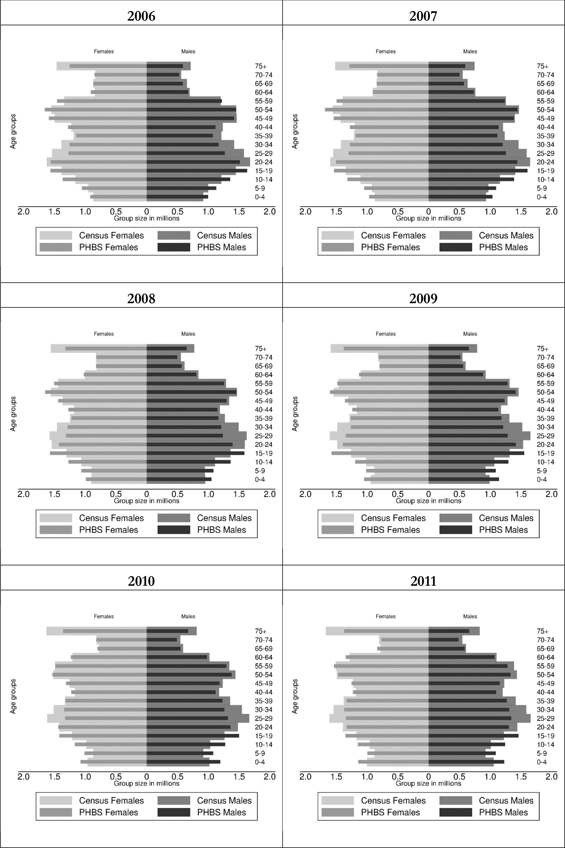
As we can see from Table 2, the gross population of Poland in PHBS data using the CSO baseline weights accounts for about 98–99% of the total population in the official statistics. This small discrepancy is partly driven by lack of survey coverage of collective dwellings and may result from definitional differences concerning residence status.3 Looking at the population distribution by age, however, suggests significant under and over-representation of some of the age groups. Details for the years covered by the analysis are given in Figure 1 in the form of population pyramids by 5- year age groups. The dark-coloured bars represent the PHBS population, while the lighter coloured are the census-based official statistics. In all years that we examine we find over-representation of children and under-representation of those aged 20–49 in the PHBS data relative to external statistics, both among men and women. There is also some under-representation of the oldest groups of the population.

Population age structure in baseline PHBS and demographic CSO statistics: 2006–2011.
Source: Baseline PHBS 2006–2011 and external statistics (see endnote 2 for sources).
This difference in the demographic structure of the population is surprising. Some of the discrepancy among older individuals could be explained by lack of coverage of collective dwellings like hospitals or retirement homes, although the latter are not very common in Poland and lack of coverage of collective dwellings in the survey affects other age groups as well. Lower numbers among those of working age could be partly related to temporary migrations. In case of children, there is however no obvious reason for the discrepancies other than over-representation of families with children in the survey.
Table 2 suggests also that the PHBS under-represents individuals with higher education. This under-representation is as high as 21%–27% for years 2006–2010 relative to other official statistics, but falls to only about 6% in 2011. In Table 3 we can see that relative to external statistics employees are over-represented in the sample by between 10–15% and the self-employed are under- represented, in particular in more recent years of data. We return to these two issues in the discussion of the factors we consider in the re-weighting process in Section 4. The PHBS data from years prior to 2010 significantly over-represents farmers which may be caused by definitional problems in survey and administrative data, but probably reflects also the fact that weights prior to 2010 were based on the 2002 Farming Census and the structure of farming in Poland saw substantial changes since then. The data beginning with 2010, with weights based on the 2010 Farming Census and the 2011 National Census, are much closer to other administrative records on the number of farmers. In Table 3 in addition to employment status comparisons we also present the correspondence of the PHBS data with administrative records with regard to the number of recipients of the main Social Security benefits. The correspondence of these numbers to official statistics differs in different years, but the numbers are generally close. The main exception are Family Pensions, which seem to be underreported by up to 26%. The most likely reason behind it is reporting accuracy related to the precise naming of pensions, which we discuss in Section 4.
The values presented in Table 4 compare direct output from the SIMPL microsimulation model to administrative statistics on the main elements of the tax and benefit system. We present the simulated number of individuals contributing to Social Security (SSC), Health Insurance (HI) and Personal Income Tax (PIT), and the number of recipients of Family Benefits including the principal Family Allowance (FA) and four main supplements (for large families: SLF, for starting school: SSS, for child birth: SCB, and education of disabled children: SEDC). In the case of each year we use the SIMPL microsimulation model to simulate the baseline tax and benefit system which operated in that year. Within the HI and PIT categories we show the total number of contributors and additionally list the numbers by those paying contributions on permanent employment and self-employment income. For PIT we also give the numbers of recipients of the Child Tax Credit, a generous tax credit for families with children introduced in 2007.
Simulated numbers for Social Security contributions are relatively close to the official figures, with an overestimate of 6.3% in 2011. As in the case of the employment status we overestimate Health Insurance contributions for the employees (by between 10% and 21%) and underestimate them for the self-employed (by 7%–17%). The number of people paying income taxes, on the other hand, overall matches relatively well with administrative statistics. However, since we are unable to account for the details of tax deductions among the self-employed, and cannot identify clearly the specific ways people file their taxes, the number of tax payers in this category is substantially higher compared to the official statistics. Given the over-representation of children in the data it is not surprising that the model significantly overestimates the number of recipients of the Child Tax Credit as well as the means-tested Family Benefits. In the latter case the basic Family Allowance is overestimated by about 32% in 2006 and by 17% in 2011, while the supplement to large families by as much as 104% in 2006 and 40% in 2011. Some of this overestimation might reflect non-take up, but the differences between supplements suggest that while the data generally over-represents families with children, it might be over-representing households with a high number of children to a much larger extent than households with one or two children.
4. Weight calibration
In the weight calibration exercise we take the age distribution as the primary source of external data with respect to which the baseline weights are adjusted. This is then supplemented with information on a number of income sources and finally with a combination of selected income sources and a small number of variables simulated in the microsimulation model. The weight calibration exercise follows the approach of Vanderhoeft (2001) and Creedy (2004) described also in Deville and Sarndal (1992).
The main principle of the approach is that it assumes validity of the “target” data to which the weights are calibrated. The calibration procedure does not change the observations themselves. Instead, it changes the household weights in such a way as to represent different aggregated population characteristics in the best possible way, taking into account a “minimum-distance” criterium which minimizes the sum of differences between the old and new weights. Having variables and observations, we have a vector xjk, where j = 1, 2, …, m and k = 1, 2, …, n. We can then define population totals for every variable such that
The goal of the exercise is to minimise the distance wkG(·), where G(·) is a distance function:
subjected to m calibration constraints:
where wk are the new calibrated weights equal to wk = gkdk, with gk representing the factors by which baseline weights are adjusted, and t′k are the target population totals, set as targets for the calibration exercise.
Different distance functions can be used for the calibration procedure. The approach used here follows the Deville-Sarndal distance function (Deville & Sarndal, 1992), that eliminates negative weights and constrains the new weights so that they do not exceed a specified lower and upper bound, relative to the old weights. The optimization problem (1) constrained by (2) is solved numerically (for more details on properties of different distance functions see: Deville & Sarndal, 1992, Vanderhoeft, 2001 and Creedy, 2004). Calibration procedure according to the above methodology is available in Stata in the REWEIGHT package of Pacifico (2010). The Deville and Sarndal (1992) distance function allows setting the minimum and maximum factors by which new weights may differ relative to the old ones, and the package permits automatic adjustment of these values once the initial factors prove too restrictive for the iterative algorithm.
4.1 Three stages of calibration
There is clearly an endless number of ways in which weight calibrations could be conducted, conditional on the choice and number of target variables as well as specific methods of calibration. Below we list a number of factors which we take into account to guide the calibration process. While the exercise conducted in the paper is specific to Polish data and the microsimulation model we use, the outlined process and the factors considered are more general and could be applied to other datasets and country scenarios. As we argue, it is clear that the accuracy of microsimulation relies on the quality of the micro-level data and the quality of the microsimulation model itself. However, the assessment of this quality depends on several other important factors, in particular on the accuracy and coverage of external statistics one uses to compare the results to, and on the definitional correspondence between survey data and these statistics. The analysis in this paper refers to the following six factors:
representativeness of the survey;
accuracy of external statistics;
definitional correspondence between survey data and external statistics;
reporting accuracy of the survey;
coverage of external statistics;
accuracy of microsimulation.
Representativeness of the survey is crucial for accuracy of the results, and the first indication of problems with it are the discrepancies between the age distribution in the survey data and in population statistics. The latter take the National Census as the starting point and are then regularly updated from population registries. Since definitional correspondence and reporting accuracy should not be a problem when it comes to age, we use the information from external statistics and adjust the age distribution to correct the representativeness of the PHBS in each of the re-weighting stages. The only factor that might affect the validity of the comparison of age distributions is lack of coverage of individuals living in collective dwellings. These individuals are covered by general population statistics but are not present in the PHBS. However, the proportion of individuals in collective dwellings in Poland is low (according to the 2011 Census it is only about 0.95% of the overall population), and so this should not significantly affect the results, in particular that the re- weighting is done in such a way that the total grossed-up population is the same before and after adjustment.
As we saw in Table 2 there are also significant differences between the survey data and external statistics when it comes to education information, and in principle it would seem natural to include education as one of the targets for re-weighting. In this case, as in the case of age, there should be good definitional correspondence and also high reporting accuracy in the survey. However, in the case of education there seems to be a problem with reliability of external statistics which can serve as a note of caution against taking them for granted. The values for 2006–2010 given in Statistical Yearbooks were calculated based on the 2002 Census and updated with local registry data and educational surveys. For these years the discrepancy between the survey and external statistics for higher education is as high as 27% in 2007 (see Table 2). However, once the reference changed to the 2011 Census data, the degree of overestimation of the number of individuals with higher education in the PHBS falls to only about 6%. This suggests that for the earlier years it is the survey, rather than the (estimated) official statistics, that give a more accurate picture of the education distribution. We therefore do not use education as a weight calibration target in our analysis.
A good example reflecting problems with reporting accuracy in the survey is the discrepancy we observe for family pensions (see Table 3). The most likely explanation behind the differences we observe in the data is that these pensions include survivors’ pensions which in the survey are likely to be declared by surviving spouses of retirement age as retirement pensions. This is consistent with the small over-representation of retirement pensions in the data and the close correspondence of survey data and external statistics when we include all the pensions together. Thus in this case, while it is possible to set the number of recipients of each individual category of pensions as target for calibration, it may be preferable to target the total number of pension recipients.
Given the statistics provided in Table 2 one could also suggest re-weighting with the use of employment status as one of the target variables. This instance is, however, an example of potential lack of definitional correspondence with an unclear split between employees and the self-employed. In Poland many individuals, for tax optimization purposes, are officially self-employed but perform their tasks in a way which has all the features of contractual employment. In this case it is possible that in the survey they may report the latter, while in the official statistics they will figure as self- employed. Additionally, reliability of external statistics on the number of employees and self- employed combines information from another survey (the Polish Labour Force Survey) and other estimates for the national accounts, which could also be problematic. In this case we therefore decided to target outcomes which may be less prone to definitional discrepancies between the survey and official statistics and use the information on health insurance and income tax contributions matched with simulated obligations to pay these using our microsimulation model.4
Definitional correspondence is also affected by the time-span of the survey and the time covered by external statistics. In the case of the PHBS the data collected for a particular household covers the period of one month, and thus ideally the database should be related to external statistics expressed in (average) monthly terms. In this regard headcount measures are particularly likely to be sensitive to different time coverage. For example, in the case of the number of recipients of a particular source of income (e.g. disability pension) the survey will record information on all regular recipients but will miss some of the individuals receiving this income on irregular basis, since the data for some of such households may be collected in months when they do not receive this income. When compared to overall annual headcount data in such cases the grossed up number of recipients in the survey will be lower compared to annual external statistics. For our analysis we use a number of external (average) monthly statistics on such variables as income sources from social security and social security contributions. If such monthly statistics do not exist, as for example in the case of the number of income tax payers, we then have to rely on a comparison with annual information.
When, as in the case of comparing insurance contributions, we use microsimulation output as a target variable in the re-weighting process we have to assume that the calculations performed in the model are correct. Realizing the complexity of tax and benefit systems, we understand that this is a strong assumption, indeed an assumption which is regularly tested by comparing external statistics to the output of the models. On the other hand, such factors as closer definitional correspondence of the target variables and availability of comparable administrative information would favour using microsimulation output for re-weighting. An important issue in this regard is to choose microsimulation targets for which the risk of errors in generating the relevant information in the microsimulation model is low. If used cautiously microsimulation output could be a valuable reference for re-weighting. Below we use results of microsimulation in the third stage of re-weighting taking the number of identified individuals paying taxes or health insurance. We also show an extended example of using more detailed microsimulation output in Section 5.4 where for 2011 we use information on joint taxation to re-weight the number of high earners in the data.
The calibration exercise is conducted in three stages. At each stage we use a specified set of target variables and the same calibration method for every year of data. The target variables used at each stage of calibration are given in Table 5.
Summary of calibration targets.
| System | Target variables | Description |
|---|---|---|
| S0 | – | Baseline weights |
| S1 | Household size | 6 groups by household size (1, 2, 3, 4, 5, 6+); |
| Place of residence | 2 groups: rural or urban; | |
| Age | 16 groups by 5 year threshold; | |
| S2: | S1 + recipients of 7 income sources (as declared in PHBS) | employee: permanent and temporary; self employment; pensions: pre-retirement, retirement, disability and family pensions; unemployment benefit; |
| S3: | S1 + recipients of 2 income sources: (as declared in PHBS) + SIMPL output: | all pensions; unemployment benefit; number of contributors to: Personal Income Tax; Health Insurance on permanent employment; Health Insurance on self-employment; |
In each of the three calibration stages we target two principal variables which underlie the generation of baseline weights at the CSO relating to the household size and the place of residence (see Section 2). These target variables are generated from the data using the baseline weights so that they remain unchanged in the calibration. The additional criterion on which weights are calibrated in Stage 1 (S1) are demographic targets related to age distribution. Stage 2 (S2) extends these targets by adding seven types of basic income sources as declared in the PHBS. Finally in Stage 3 (S3), instead of these seven income sources we use two indicators for income receipt in which case there should be high degree of definitional correspondence, namely receipt of any social security pension and unemployment benefit, and supplement this by a number of outcome variables from the microsimulation model. These targets are the number of individuals paying Personal Income Tax and employee and self-employed Health Insurance. The starting weights for the calibration exercise are the baseline weights as provided by the CSO. Results generated using these baseline weights are labelled as S0. Re-weighting in this paper has been considered as a technical approach to assist the process of producing better quality policy analysis. The three stages of calibration reflect a complex process of choosing relevant targets as well as benchmarks to validate the results.
5. Results
5.1 Effects of re-weighting: PHBS data and microsimulation outcomes
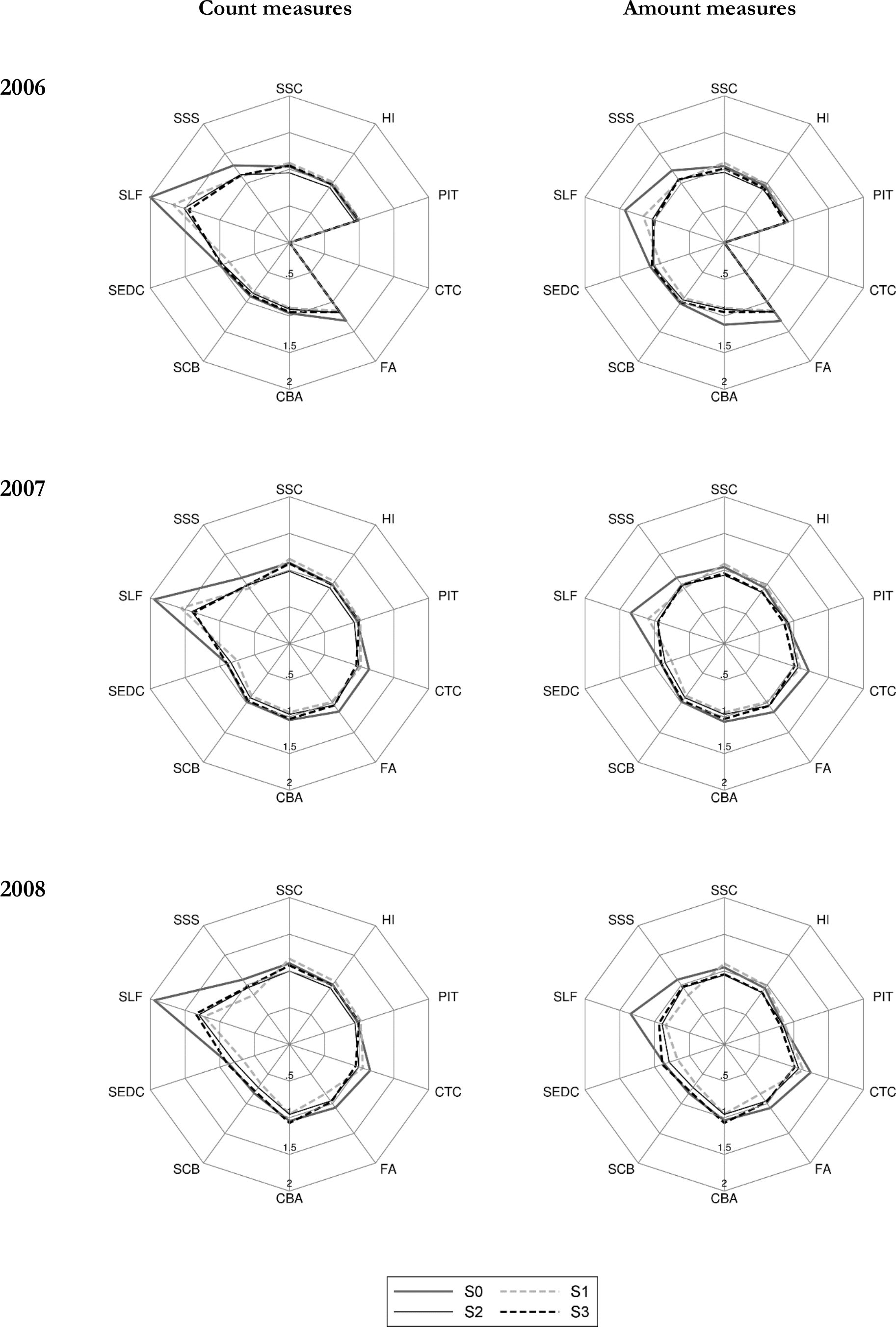
The effect of weight calibration under the above three scenarios is presented in two categories. First, we show how the calibrations affect the correspondence of economic status and social security benefit receipt relative to external data, and secondly, we present aggregate outcomes of the microsimulation model as compared to administrative statistics. In a similar way to the detailed results presented in Table 4, for each of the years considered in the analysis we apply the baseline tax and benefit system for the given year. The differences between S0 and S1–S3 in the grossed-up number of individuals in specific economic status and social security benefit receipt category as well as with regard to the simulation outputs, result purely from changes in the values of weights. The results in the form of ratios of PHBS based figures and external sources for the economic status and SSC benefit receipt are presented in Table 6. The amount figures for the simulated contributions and tax outcomes are shown in Table 7, while for Family Benefits in Table 8. For these parameters we also show the ratios between the simulated and administrative information for headcount and aggregate amounts in the form of radar charts in Figures 2 and 3 (generated using radar graphs for Stata, Mander, 2007). The tables and figures include the same tax and benefit outcomes as those chosen for the baseline validation presented in Table 4. The closer the relative values are to 1, the closer are the simulated values to their administrative counterparts. The list of the tax and benefit parameters and their labels is given in Table 9.

Macrovalidation results: Selected tax and benefit outcomes using different weights (S0, S1, S2, S3): 2006, 2007 and 2008 relative to administrative data.
Source: SIMPL model on PHBS 2009–2011 and external statistics (see endnote 2 for sources).
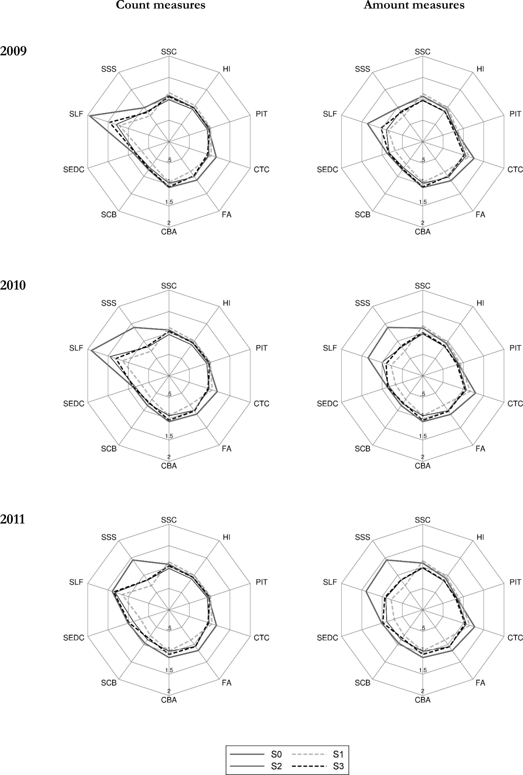

Macrovalidation results: selected tax and benefit outcomes using different weights (S0, S1, S2, S3): 2009, 2010 and 2011 relative to administrative data
Source: SIMPL model on PHBS 2009–2011 and external statistics (see endnote 2 for sources).
PHBS and external statistics: Ratios of income sources (headcount) by weight calibration for 2006–2011.
| Income source and weights | 2006 | 2007 | 2008 | 2009 | 2010 | 2011 |
|---|---|---|---|---|---|---|
| Permanent employment | ||||||
| S0 | 1.159 | 1.196 | 1.194 | 1.183 | 1.200 | 1.198 |
| S1 | 1.222 | 1.261 | 1.267 | 1.264 | 1.273 | 1.271 |
| S2 | 1.000 | 1.000 | 1.000 | 1.000 | 1.000 | 1.000 |
| S3 | 1.085 | 1.062 | 1.030 | 1.034 | 1.036 | 1.031 |
| Temporary employment | ||||||
| S0 | 1.921 | 1.621 | 1.491 | 1.299 | 1.041 | 0.810 |
| S1 | 1.971 | 1.647 | 1.498 | 1.267 | 1.009 | 0.792 |
| S2 | 1.000 | 1.000 | 1.000 | 1.000 | 1.000 | 1.000 |
| S3 | 3.483 | 3.759 | 3.691 | 3.389 | 2.690 | 2.097 |
| Self employment | ||||||
| S0 | 0.702 | 0.729 | 0.693 | 0.739 | 0.758 | 0.746 |
| S1 | 0.706 | 0.733 | 0.699 | 0.749 | 0.770 | 0.770 |
| S2 | 1.000 | 1.000 | 1.000 | 1.000 | 1.000 | 1.000 |
| S3 | 0.779 | 0.839 | 0.830 | 0.860 | 0.887 | 0.922 |
| Farmer | ||||||
| S0 | 1.314 | 1.239 | 1.164 | 1.125 | 0.989 | 0.914 |
| S1 | 1.392 | 1.333 | 1.253 | 1.220 | 1.071 | 1.001 |
| S2 | 1.678 | 1.715 | 1.646 | 1.590 | 1.475 | 1.326 |
| S3 | 1.471 | 1.472 | 1.433 | 1.458 | 1.230 | 1.161 |
| Retirement pension | ||||||
| S0 | 1.038 | 1.023 | 1.043 | 1.040 | 1.030 | 1.033 |
| S1 | 1.071 | 1.077 | 1.092 | 1.085 | 1.086 | 1.085 |
| S2 | 1.000 | 1.000 | 1.000 | 1.000 | 1.000 | 1.000 |
| S3 | 1.053 | 1.061 | 1.069 | 1.063 | 1.067 | 1.071 |
| Disability pension | ||||||
| S0 | 1.048 | 1.021 | 1.009 | 0.986 | 0.967 | 0.972 |
| S1 | 1.050 | 1.034 | 1.025 | 1.020 | 0.995 | 1.011 |
| S2 | 1.000 | 1.000 | 1.000 | 1.000 | 1.000 | 1.000 |
| S3 | 1.007 | 0.999 | 1.012 | 1.013 | 0.992 | 0.998 |
| Family pension | ||||||
| S0 | 0.862 | 0.826 | 0.763 | 0.754 | 0.747 | 0.735 |
| S1 | 0.849 | 0.817 | 0.739 | 0.722 | 0.728 | 0.715 |
| S2 | 1.000 | 1.000 | 1.000 | 1.000 | 1.000 | 1.000 |
| S3 | 0.806 | 0.763 | 0.709 | 0.724 | 0.709 | 0.698 |
| Pre-retirement pension | ||||||
| S0 | 0.990 | 1.005 | 0.914 | 0.891 | 1.030 | 0.981 |
| S1 | 0.936 | 0.963 | 0.889 | 0.881 | 1.046 | 1.009 |
| S2 | 1.000 | 1.000 | 1.000 | 1.000 | 1.000 | 1.000 |
| S3 | 0.902 | 0.921 | 0.882 | 0.818 | 1.038 | 0.936 |
| Unemployment benefit | ||||||
| S0 | 0.867 | 0.884 | 0.830 | 0.909 | 0.855 | 0.793 |
| S1 | 0.880 | 0.900 | 0.845 | 0.952 | 0.886 | 0.812 |
| S2 | 1.000 | 1.000 | 1.000 | 1.000 | 1.000 | 1.000 |
| S3 | 1.000 | 1.000 | 1.000 | 1.000 | 1.000 | 1.000 |
-
Source: PHBS data 2006–2011 and external statistics (see endnote 2 for sources), weighted with baseline (S0) and calibrated (S1–S3) weights.
PHBS and external statistics: Ratios of contributions and taxes (amount) in SIMPL by weight calibration for 2006–2011.
| Simulation output and weights | 2006 | 2007 | 2008 | 2009 | 2010 | 2011 |
|---|---|---|---|---|---|---|
| Social security contribution (SSC) | ||||||
| S0 | 1.041 | 1.042 | 1.049 | 1.061 | 1.114 | 1.092 |
| S1 | 1.089 | 1.085 | 1.102 | 1.122 | 1.167 | 1.145 |
| S2 | 0.959 | 0.930 | 0.944 | 0.962 | 0.977 | 0.974 |
| S3 | 1.009 | 0.955 | 0.955 | 0.966 | 1.007 | 0.989 |
| Health insurance contributions (HI) | ||||||
| S0 | 0.954 | 0.937 | 0.945 | 0.940 | 0.937 | 0.913 |
| S1 | 0.985 | 0.971 | 0.985 | 0.985 | 0.977 | 0.952 |
| S2 | 0.899 | 0.865 | 0.873 | 0.872 | 0.852 | 0.839 |
| S3 | 0.922 | 0.873 | 0.878 | 0.876 | 0.869 | 0.851 |
| Personal Income Tax (PIT) | ||||||
| S0 | 0.917 | 0.901 | 0.843 | 0.812 | 0.882 | 0.849 |
| S1 | 0.920 | 0.926 | 0.869 | 0.854 | 0.922 | 0.892 |
| S2 | 0.919 | 0.923 | 0.844 | 0.816 | 0.872 | 0.843 |
| S3 | 0.875 | 0.866 | 0.808 | 0.775 | 0.844 | 0.818 |
| Child Tax Credit (in PIT) | ||||||
| S0 | – | 1.214 | 1.241 | 1.262 | 1.299 | 1.278 |
| S1 | – | 1.092 | 1.133 | 1.135 | 1.168 | 1.159 |
| S2 | – | 1.059 | 1.070 | 1.063 | 1.073 | 1.071 |
| S3 | – | 1.008 | 1.011 | 1.020 | 1.040 | 1.040 |
-
Source: PHBS data 2006–2011 and external statistics (see endnote 2 for sources), weighted with baseline (S0) and calibrated (S1–S3) weights.
PHBS and external statistics: Ratios of Family Benefits (amount) in SIMPL by weight calibration for 2006–2011.
| Simulation output and weights | 2006 | 2007 | 2008 | 2009 | 2010 | 2011 |
|---|---|---|---|---|---|---|
| Family Allowance (FA) | ||||||
| S0 | 1.319 | 1.154 | 1.072 | 1.124 | 1.112 | 1.174 |
| S1 | 1.149 | 0.988 | 0.835 | 0.873 | 0.843 | 0.872 |
| S2 | 1.174 | 1.045 | 0.960 | 1.024 | 1.004 | 1.059 |
| S3 | 1.164 | 1.049 | 0.976 | 0.999 | 1.023 | 1.062 |
| Family Allowance supplements: | ||||||
| - large families (SLF) | ||||||
| S0 | 1.425 | 1.344 | 1.344 | 1.359 | 1.346 | 1.397 |
| S1 | 1.162 | 1.093 | 0.841 | 0.848 | 0.781 | 0.779 |
| S2 | 1.032 | 0.960 | 0.891 | 0.895 | 1.005 | 0.910 |
| S3 | 1.003 | 0.949 | 0.937 | 1.026 | 0.901 | 0.935 |
| - starting school (SSS) | ||||||
| S0 | 1.216 | 1.107 | 1.089 | 0.980 | 1.395 | 1.441 |
| S1 | 1.045 | 0.931 | 0.831 | 0.747 | 0.710 | 0.701 |
| S2 | 1.069 | 0.980 | 0.956 | 0.879 | 0.833 | 0.856 |
| S3 | 1.062 | 0.983 | 0.971 | 0.850 | 0.859 | 0.864 |
| - child birth (SCB) | ||||||
| S0 | 1.024 | 0.984 | 0.822 | 0.810 | 0.857 | 0.960 |
| S1 | 0.935 | 0.883 | 0.665 | 0.657 | 0.680 | 0.741 |
| S2 | 0.964 | 0.913 | 0.727 | 0.756 | 0.803 | 0.858 |
| S3 | 1.004 | 0.963 | 0.793 | 0.790 | 0.780 | 0.814 |
| - education of disabled child (SEDC) | ||||||
| S0 | 1.063 | 0.904 | 0.862 | 0.874 | 0.866 | 1.009 |
| S1 | 0.919 | 0.758 | 0.671 | 0.681 | 0.669 | 0.702 |
| S2 | 1.020 | 0.849 | 0.790 | 0.828 | 0.825 | 0.885 |
| S3 | 1.039 | 0.904 | 0.890 | 0.838 | 0.864 | 0.982 |
| Child Birth Allowance (CBA): | ||||||
| S0 | 1.119 | 1.067 | 1.037 | 1.069 | 1.070 | 1.112 |
| S1 | 0.891 | 0.939 | 0.951 | 0.949 | 0.934 | 0.957 |
| S2 | 0.908 | 0.966 | 0.955 | 0.970 | 0.932 | 0.964 |
| S3 | 0.947 | 1.028 | 1.072 | 1.053 | 1.036 | 1.038 |
-
Source: PHBS data 2006–2011 and external statistics, weighted with baseline (S0) and calibrated (S1–S3) weights.
Elements of tax and benefit used as performance measures.
| Abbreviation | Full name |
|---|---|
| Taxes and contributions | |
| SSC | Social Security Contributions |
| HI | Health Insurance contributions |
| PIT | Personal Income Tax |
| CTC | Child Tax Credit (within PIT) |
| Family Benefits: | |
| FA | Family Allowance |
| SCB | FA Supplement for Child Birth |
| SEDC | FA Supplement for Education and Rehabilitation of Disabled Child |
| SLF | FA Supplement for Large Families |
| SSS | FA School Starting Supplement |
| CBA | Child Birth Allowance |
As shown in Tables 7 and 8 and summarized in Figures 2 and 3, weight calibration generally leads to an improved correspondence in the results for most of the selected simulated parameters. The most significant improvements apply to the Family Allowance and its supplements. The biggest relative deviation from the administrative data can be observed in the Supplement for Large Families (SLF) which is oversimulated by over 100% in 2006 in terms of the headcount measure and by 43% in terms of amount when using baseline weights. For all calibration targets in a given period the number of recipients and the aggregate value of the SLF drops substantially and gets closer to the administrative records. The headcount values are still oversimulated but by much less compared to the baseline weights. In terms of total spending most of the simulations generate results closely matching the administrative values. A similar picture can be seen for the Supplement for Starting School (SSS) in years 2010 and 2011.
The results on the contributions side are not as straightforward, and there are important differences between the accuracy of results by headcount and aggregate amounts. Figures 2 and 3 show that, as we would expect given the target variables in S2 and S3, the second and third stage of the calibration substantially improve the respective number of contributors to Social Security and Health Insurance and taxes. This is the result of calibrating the number of recipients of the main types of incomes in S2 and of selected types of contributions in S3. The improvements in terms of aggregate amount of contributions and taxes are less clear cut. The details are presented in Table 7 and we can see that often, while there are improvements in terms of the numbers of contributors to Social Security, the calibrations result in slightly higher deviations in terms of aggregate amounts of Health Insurance and income taxes. The reason behind this is that when we target income sources or the number of social insurance contributions we risk lowering the weight on top income recipients in the data who generate a significant proportion of tax and contributions incomes. In Section 5.4 we propose an alternative calibration approach which extends the use of microsimulation output to re-weight high income households and, as a result, produces a further improvement relative to administrative data.
5.2 Cumulative assessment of re-weighting
The final issue we address is an overall assessment of the quality a particular re-weighting exercise. In this we follow the methods often used in the assessment of forecast accuracy and generate a distance measure based on percentage errors for a select number of microsimulation outcome measures.5 The measure we use is the Root Mean Squared Percentage Error computed on a selected number of key microsimulation results relative to administrative statistics. Percentage scales seem more suitable in our case compared to absolute values as in the case of many microsimulation outcomes we are faced with different orders of magnitude. For example about 2.8 million children received the Family Allowance and only 0.2 million received the Supplement for Child Birth in 2011. The Root Mean Squared Percentage Error is defined as:
where l is the number of tax and benefit outcomes included in the analysis (as presented in Table 9), and si is the ratio of simulated to administrative values for that particular outcome. These indicators are computed separately for the headcount measure and for aggregate amounts of taxes and benefits.
In our exercise we focus on some key elements of the tax and benefit system and to assess the combined accuracy of the model we include the Social Security Contributions, Health Insurance, Personal Income Tax values and the Family Allowance with the most important supplements. The summary of the comparison for the chosen set of parameters is presented in Figure 4. The results reflect our detailed discussion and show overall significant improvements in the accuracy of simulations, especially for Stages 2 and 3. Improvements in the aggregate measures are substantial even despite the slightly less precise results on insurance and income taxes in a number of cases. The indicator with calibrated weights is higher compared to the baseline only in the case of amounts for S1 calibrations in 2008 and 2009. These results relate to a substantial under-simulation of a number of elements of the Family Benefits system in these two years. It is interesting to note that the summary indicators for the second and third stage of calibrations are very close to each other for all of the analysed years in terms of both the headcount and aggregate amounts.

Mean square relative distance measure using different weights (S0, S1, S2, S3).
Source: SIMPL model on PHBS 2006–2011 and external statistics (see endnote 2 for sources).
Additionally, as a robustness check of our method we compare the original weights to the calibrated ones to check by how much the new weights diverge. The Deville-Sarndal calibration method allows setting the maximum divergence of the new weights from the baseline numbers. In our case we initially set the weights to diverge by ratio of 2 in the upper bound and by 0.8 in the lower bound. We allowed for higher values only in the case of lack of convergence after 200 runs. In Table 10 we provide maximum and minimum values together with standard deviations for the ratio of new to old weights for every calibration stage in each year. As could be expected given the change in the number of targets, the maximum deviation is lower in the Stage 1 compared to S2 and S3, but there is no clear pattern between S2 and S3. The maximum ratio of new to old weights in the Stage 2 range from 2.6 to 5.3, while in Stage 3 from 3.2 to 5.9.
Minimum and maximum ratios of calibrated to baseline weights for calibration stages S1, S2 and S3.
| S1 | S2 | S3 | |||||||
|---|---|---|---|---|---|---|---|---|---|
| Max. | Min. | s.d. | Max. | Min. | s.d. | Max. | Min. | s.d. | |
| 2006 | 2.00 | 0.80 | (0.29) | 5.26 | 0.28 | (0.43) | 5.92 | 0.52 | (0.44) |
| 2007 | 2.00 | 0.80 | (0.32) | 4.69 | 0.33 | (0.47) | 3.96 | 0.15 | (0.55) |
| 2008 | 4.41 | 0.25 | (0.28) | 4.78 | 0.14 | (0.49) | 4.49 | 0.23 | (0.62) |
| 2009 | 2.45 | 0.44 | (0.29) | 2.62 | 0.23 | (0.47) | 5.72 | 0.38 | (0.62) |
| 2010 | 3.39 | 0.23 | (0.28) | 4.01 | 0.73 | (0.62) | 4.69 | 0.46 | (0.70) |
| 2011 | 3.04 | 0.17 | (0.28) | 3.75 | 0.40 | (0.48) | 3.16 | 0.15 | (0.62) |
| 2.00 | 0.80 | (0.29) | 5.26 | 0.28 | (0.43) | 5.92 | 0.52 | (0.44) | |
-
Source: Authors’ calculations using PHBS data 2006–2011 and external statistics (see endnote 2 for sources), weighted with baseline (S0) and calibrated (S1–S3) weights. Standard deviation in brackets.
5.3 Re-weighting and measures of income inequality
Finally, we turn to some analytical consequences of re-weighting and examine the effect of the exercise from the perspective of income inequality statistics to check if the process of re-weighting affects the level of inequality in specific years as well as whether it influences the trends in inequality developments. Inequality statistics (computed using Inqdeco, Jenkins, 1999) - the Gini coefficients and the 9/1 decile ratios, together with their 95% confidence intervals, are shown in Figure 5. Differences in inequality measures when we only calibrate the age distribution are insignificant when compared to the values obtained with baseline weights. This is not the case, however, with the two extended stages, S2 and S3. In these cases inequality indicators are substantially higher and differences with respect to measures using baseline weights are in the majority of cases statistically significant. Trends in inequality dynamics are also different for the latter two stages of calibration in particular when we consider the S3 re-weighting approach.

Inequality levels using different weights (S0, S1, S2, S3).
Source: SIMPL model on PHBS 2006–2011.
5.4 Calibrating the top end of the income distribution using joint taxation
As we saw above, while re-weighting generally improves microsimulation outcomes, in some cases the simulated results may actually diverge by slightly more for the calibrated weights compared to baseline values. In our analysis this relates, for example, to aggregate values of total income tax and is due to reduced weights on top income earners in Stages 2 and 3 of re-weighting. To address this issue we extend the use of microsimulation outcomes which can be compared to published government income tax data and use it to re-weight the top end of the income distribution to correct for under-representation of highest earners (see e.g.: O’Donoghue, Sutherland & Utili, 1999).6
In this specific example we calibrate the weights on tax advantages from joint taxation of couples. In the Polish tax code couples can file taxes jointly, in which case the tax schedule is applied to half of the total taxable income of the couple and the resulting taxes are then multiplied by two. Given the relatively low degree of progressivity in the Polish tax system, this treatment of couples brings highest benefits to high income couples with large differences in incomes between the partners, and specifically, in cases when one of the partners has incomes exceeding the higher income tax rate threshold (85,528 PLN or about 19,000 euro per year) and the other one does not.
The Polish Ministry of Finance regularly publishes the costs of the major tax advantages, including joint taxation which in 2011 cost the budget 2.98bn PLN (0.7bn euro, see Ministerstwo Finansów, 2012). The simulated costs of these advantages in the SIMPL microsimulation model using the baseline weights is only 2.20bn PLN. The re-weighting conducted here adjusts the household weights in such a way that the simulated cost of joint taxation matches closely the officially published figure. While the re-weighting targets the value of the tax advantage, the parameter included in the process specifies the number of high income earners in the population, whom we define as individuals with earnings equal to five times the official monthly average gross wage, which in 2011 was equal to 3,400 PLN (or about 770 EUR). The re-weighting therefore implies increasing the number of all high earners sufficiently to match the total cost of joint taxation.
The cost of joint taxation (JTC) can be expressed as a function of the number of people in the population (ntr) exceeding the specified income threshold (tr):
The grossed-up number of individuals in the data who have incomes higher than a chosen threshold can be changed through changes in the weights. Thus by setting a specific requirement in the re-weighting procedure to match the cost of joint taxation, the re-weighting process will increase the weights on higher earners up to the point when the simulated cost of joint taxation will match administrative records. Specifying JTC0 to be the administrative cost of joint taxation and JTCdata the cost calculated from the data, we can define our optimization problem as:
The solution involves the application of the Nelder-Mead method (Nelder and Mead, 1965), as for each set of weights we need to compare two sets of outputs from the model to specify the cost of joint taxation (one set with and one without the tax advantages).7 In each step of the Nelder-Mead optimization run we add ntr to Stage 3 as an additional calibration target and adjust weights as described previously. In effect we find weights with which the modelled total cost of joint taxation equals to that published by the Ministry of Finance. The exercise is presented only for 2011 and in this stage of calibration we use the information on joint taxation on top of the other targets used in Stage 3 for the 2011 re-weighting (we label the calculations as: S3+JTax).
The additional criterion results in improved simulation results. In Figure 6 we present the baseline results, together with results from S3 and S3+JTax. Compared with other calibration systems we see improvement in the simulation of the overall amount of personal income tax with underestimation of PIT growing from 15% using the baseline weights, to 18% with S3 weights (Table 7) and then falling to 6% if we additionally target the total cost of joint taxation. Naturally, since we increase the grossed-up number of high income households inequality measures grow further above those obtained with S3 weights. The Gini coefficient goes up significantly from 0.315 to 0.349 and the p90/p10 ratio increases from 3.725 to 4.059.

Macrovalidation results: Selected tax and benefit outcomes using different weights (S0, S1, S3, S3+JTax): 2011 relative to administrative data.
Source: SIMPL model on PHBS 2011 and external statistics (see endnote 2 for sources).
6. Conclusions and notes of caution
Calibration of grossing-up weights can result in substantial improvements in the accuracy of microsimulation results. Important gains in the performance of the Polish microsimulation model SIMPL appear already after correcting for the distribution of age (S1), which is probably the least controversial and arbitrary adjustment. Interestingly, in our application these changes are neutral from the point of view of the overall income distribution. More detailed re-weighting using indicators related to income sources (S2) and tax identifiers (S3) result in further overall improvement of the accuracy of microsimulation, and these significantly change the distribution of income in terms of the level of inequality and also affect the pattern of changes in inequality over time.
One should approach re-weighting of data with caution and bear in mind a set of important factors. First of all, it is important to identify the most likely reasons for the observed discrepancies between the survey data and external statistics, in particular taking into account the way the survey weights are constructed. It needs to be noted as well that the comparison will be affected not only by the representativeness of the survey but also by such factors as accuracy of external statistics, definitional correspondence between survey data and external statistics, reporting accuracy of the survey and coverage of external data. In the Polish case as far as the age distribution is concerned, we can count on reliable and directly comparable external data, and there is also little reason for definitional discrepancy or survey reporting inaccuracies. In such cases the most likely reason for discrepancies is selective survey non-response with respect to these characteristics and the fact that baseline weights do not account for it. Adjusting the weights in such cases, in particular if it also accounts for categories taken into consideration in generating the baseline weights, seems justified, and as we saw in Section 5, might bring substantial gains in the accuracy of simulation results.
When there are reasons to believe that discrepancies between survey and external data are consequences of factors other than survey representativeness, one should approach reweighting with a degree of caution. Our analysis pointed out examples of discrepancies which are most likely results of other factors we considered. These other factors affected the comparisons of the number of recipients of family pensions (survey reporting accuracy), number of people with higher education (accuracy of external statistics) and employment status (definitional correspondence).
In the third stage of re-weighting and in the additional exercise presented in Section 5.4 we used microsimulation output to re-weight the data. This approach needs to assume accuracy of the microsimulation output at the level of individual households, and we argued that one should only use it in cases when the scope for computational error is small and when the benefits of using microsimulation output outweigh the possible costs. This will for example be the case when there are problems with finding high quality external data to compare the survey to, in particular in the case of problems with the factors outlined above. For example, in our analysis in Stage 3 of re- weighting, we only used the number of contributors to Health Insurance identified in microsimulation analysis, rather than its aggregate values. From this point of view the third stage of re-weighting might be seen as a trade-off between using more directly comparable data on contributions at the cost of having to take advantage of microsimulation information. In the extension of Stage 3 we showed that using more detailed microsimulation output, in this case the aggregate value of tax advantages from joint taxation, can bring further benefits in terms of microsimulation accuracy. In such cases however, one has to be aware that any error in microsimulation might have substantial consequences for the accuracy of the model in respects other than the targeted outcome.
The final note of caution relates to the issue of the effect of re-weighting on the so called residual groups, i.e. groups of the population which are largely missing from the specified calibration targets. The best example of such groups in our case are farmers. The potential definitional discrepancies and lack of accuracy of external data which we discussed in Section 3, is the main reason why we leave them out of the calibration process, but the comparison of Stage 2 and 3 of re-weighting very clearly reflects the effects of calibrating a high number of targets (in Stage 2) on this residual group. We can see for example in Table 6 that the second stage of the calibration has a very substantial effect on the number of farmers in the data, with much less pronounced implications of using the smaller set of calibration targets under Stage 3.
Re-weighting ought to take into account a number of factors relating to the way survey data is collected and the nature of external statistics. As the exercise in this paper shows, careful approach to data re-weighting may significantly improve accuracy of microsimulation and thus make the analysis much better suited for the purpose of policy analysis. Various approaches to re-weighting are possible and some of them will have substantial consequences for the resulting distribution of income in the survey data and the implied levels and trends in inequality. Such differences in the distribution of income resulting from re-weighting in our view deserve further careful analysis.
Footnotes
1.
For discussion on stratified sampling see: Cameron and Trivedi, 2005.
2.
Information on age composition for 2006 and 2007 was taken from the CSO Demographic Yearbook (Główny Urząd Statystyczny, 2006–2007). For the years 2008 – 2010 from population reports as of 30 June (Główny Urząd Statystyczny, 2008–2010) and for 2011 from the National Census report (Główny Urząd Statystyczny, 2011). Data on employment, pensions, education and place of residence can be found in the Polish Statistical Yearbooks (Główny Urząd Statystyczny, 2006–2011a; Główny Urząd Statystyczny, 2006–2011b). More details on pensions are obtained from the Social Insurance Institution (ZUS) reports (Zakład Ubezpieczen Społecznych, 2006–2011). Information on Personal Income Tax were obtained from the Polish Ministry of Finance reports (Ministerstwo Finansów, 2006–2011). Data on Family Allowance was taken from the Polish Ministry of Labour and Social Policy reports (Ministerstwo Pracy i Polityki Społecznej, 2006–2011), and data on health insurance and some detailed social security statistics is taken from unpublished sources from ZUS - we are very grateful for making these available.
3.
For details see: Nowak (2013) and Główny Urząd Statystyczny (2011). Persons reported in the census data are counted as residents based solely on their presence in the local authority registers. Thus e.g. migrants who did not bother to sign out from the register are counted as still living in Poland. This may be an issue with more than 1 million migrants who left Poland after EU accession who are still being counted as living in Poland where they are actually making money and paying their taxes abroad. The official statistics published in the Demographic Yearbooks are based on the 2002 and 2010 Census results with remaining years being updated with data from local administration registers.
4.
Another problematic issue for the comparison is also the degree of employment in the shadow economy. This has been estimated to be around 800,000 in 2010 (Główny Urząd Statystyczny, 2011b). However, many of these individuals could combine official and unofficial employment, and it is also likely that unofficial employment would not be declared in the survey. We thus treat all declared employment in the data as official employment.
5.
For discussion of forecast assessment accuracy measurement see, e.g.: Armstrong and Collopy (1992) or Makridakis and Hibon (1998).
6.
There is a number of approaches for correcting under-representation of top incomes. One could, for example, correct it by fitting the tail of income distribution to Pareto distribution (e.g.: Brzezinski & Kostro, 2010). Another way is to compare centiles of the distribution in the data with published detailed information on the distribution of income from specific sources. The latter adjustment - which could also be included in the re-weighting procedure is not possible in Poland due to lack of officially published statistics on centiles of gross incomes.
7.
The Nelder-Mead method is a numerical algorithm for finding local minima of an N-dimensional function by evaluating function values at N+1 points. As a heuristic search algorithm it does not require calculations of numerical derivatives and thus requires lower number of function calls compared to other gradient optimization algorithms. It is implemented in Stata as an option in the optimize() command in Mata.
References
-
1
Error Measures For Generalizing About Forecasting Methods: Empirical ComparisonsInternational Journal of Forecasting 8:69–80.
-
2
As SIMPL As That: Introducing a Tax-Benefit Microsimulation Model for Poland. IZA Discussion Papers 2988Bonn: Institute for the Study of Labor (IZA).
-
3
Micro-simulating Child Poverty in Great Britain in 2010 and 2020. Working Paper 06–31National Poverty Centre.
- 4
- 5
-
6
Accounting For Population Ageing In Tax Microsimulation Modelling By Survey Reweighting. Australian Economic Papers18–37, Accounting For Population Ageing In Tax Microsimulation Modelling By Survey Reweighting. Australian Economic Papers, 45, 1.
- 7
-
8
Survey Reweighting for Tax Microsimultaion ModelingResearch on Economic Inequality 12:229–249.
-
9
Reweighting Household Surveys for Tax Microsimulation Modelling: An Application to the New Zealand Household Economic SurveyAustralian Journal of Labour Economics 7:71–88.
-
10
Calibration Estimators in Survey SamplingJournal of the American Statistical Association 87:376–382.
-
11
Grossing-up revisitedIn: R Hancock, H Sutherland, editors. Microsimulation Models for Public Policy Analysis: New Frontiers. London: London School of Economics and Political Science. pp. 121–132.
- 12
- 13
-
14
Rocznik Statystyczny Rzeczpospolitej PolskiejWarszawa: Zakład Wydawnictw Statystycznych.
-
15
Ludność. Stan i struktura w przekroju terytorialnymWarszawa: Departament Badań Demograficznych.
-
16
Metodologia badania budżetów gospodarstw domowychWarszawa: Departament Warunków Życia.
- 17
-
18
Wyniki wstępne Narodowego Spisu Powszechnego Ludności i Mieszkań 2011Warszawa: Zakład Wydawnictw Statystycznych.
-
19
Multi-family households in a labour supply model: a calibration method with application to PolandApplied Economics 44:2907–2919.
-
20
Statistical Software ComponentsINEQDECO: Stata module to calculate inequality indices with decomposition by subgroup, Statistical Software Components, Boston College Department of Economics.
-
21
Statistical inference in micro-simulation models: incorporating external informationMathematics and Computers in Simulation 59:255–265.
-
22
Survey nonresponse and the distribution of incomeThe Journal of Economic Inequality 4:33–55.
- 23
-
24
Evaluating Accuracy (or Error) Measures. Working Paper 1995/18/TM, INSEADEvaluating Accuracy (or Error) Measures. Working Paper 1995/18/TM, INSEAD.
-
25
Statistical Software ComponentsRADAR: Stata module to draw radar (spider) plots, Statistical Software Components, Boston College Department of Economics.
-
26
Informacja dotycząca rozliczenia podatku dochodowego od osób fizycznychWarszawa: Departament Podatków Dochodowych.
- 27
-
28
Informacja o realizacji świadczeń rodzinnychWarszawa: Departament Polityki Rodzinnej.
- 29
-
30
‘Klin’-ing up: Effects of Polish tax reforms on those in and on those outLabour Economics 17:556–566.
-
31
Financial support for families with children and its trade-offs: balancing redistribution and parental work incentivesBaltic Journal of Economics 13:59–83.
-
32
Nowcasting Indicators of Poverty Risk in the European Union: A Microsimulation Approach. EUROMOD Working Papers EM11/13EUROMOD at the Institute for Social and Economic Research.
- 33
-
34
Ludność: stan i struktura demograficzno-społeczna: Narodowy Spis Powszechny Ludności i Mieszkań 2011Warszawa: Zakład Wydawnictw Statystycznych.
-
35
Nowcasting in Microsimulation Models: A Methodological SurveyJournal of Artificial Societies and Social Simulation, 17, 4.
-
36
Integrating output in Euromod: an assessment of the sensitivity of multi country microsimulation results. EUROMOD Working Papers EM1/99EUROMOD at the Institute for Social and Economic Research.
-
37
REWEIGHT: The Stata command for survey reweighting. Center for the Analysis of Public Policies (CAPP) 0079Universita di Modena e Reggio Emilia.
- 38
-
39
Respondent Behavior in Panel Studies: A Case Study for Income- Nonresponse by Means of the German Socio-Economic Panel (GSOEP). Discussion Paper 299DIW-Berlin.
-
40
Canberra Group Handbook on Household Income StatisticsCanberra Group Handbook on Household Income Statistics, United Nations.
-
41
Generalised Calibration at Statistics Belgium: SPSS Module G-CALIB-S and Current Practices. Working Paper 3Brussels: Statistics Belgium.
-
42
Ważniejsze informacje z zakresu ubezpieczeń społecznychWarszawa: Departament Statystyki i Prognoz Aktuarialnych.
Article and author information
Author details
Acknowledgements
Michal Myck gratefully acknowledges the support of the Polish National Science Centre (NCN) under project grant number 6752/B/H03/2011/40. Mateusz Najsztub acknowledges the support of the Batory Foundation under the project number 22078. Data used for the analysis have been provided by the Polish Central Statistical Office (GUS), who take no responsibility for the results of the analysis and interpretation. The paper builds on the initial analysis conducted in the process of development of the SIMPL microsimulation model (version V4S) in cooperation with Adrian Domitrz, Leszek Morawski and Aneta Semeniuk. Their role in the development of the model has been invaluable. We would like to thank participants of the EUROMOD Research Workshop in Lisbon (October 2013) and to three anonymous referees for comments and suggestions which helped us significantly improve the paper. The usual disclaimer applies.
Publication history
- Version of Record published: April 30, 2015 (version 1)
Copyright
© 2015, Myck and Najsztub
This article is distributed under the terms of the Creative Commons Attribution License, which permits unrestricted use and redistribution provided that the original author and source are credited.