Figures and data in Distributional impacts of behavioral effects – ex-ante evaluation of the 2017 unemployment insurance reform in Finland

Cite this article as: M. Kotamäki, J. Mattila, J. Tervola; 2018; Distributional impacts of behavioral effects – ex-ante evaluation of the 2017 unemployment insurance reform in Finland; International Journal of Microsimulation; 11(2); 146-168. doi: 10.34196/ijm.00183

2 figures and 8 tables

Figures

Figure 1

Download asset Open asset

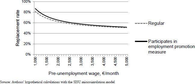
Determination of earnings-related unemployment benefit in Finland 2017.

*Source*: Authors’ hypothetical calculations with the SISU microsimulation model.

Figure 2

Download asset Open asset

Pre-reform distribution of cumulative days of earnings-related benefit by the end of 2014, percent of the recipients.

Tables

Table 1

Potential benefit durations (PBD) in the Finnish earnings-related unemployment benefit scheme before and after 2017.

	Pre-reform	Post-reform
Less than 3 years of work history	400	300
Over 3 years of work history and less than 58 years of age	500	400
Eligible for the unemployment tunnel	max 1,532	max 1,532

Source: Law on unemployment benefits, see https://www.finlex.fi/fi/laki/ajantasa/2002/20021290
Notes: The reform applies only to new unemployment spells starting from the beginning of 2017. The maximum duration of the unemployment benefits for those eligible for the unemployment tunnel assumes 258 working days a year.

Table 2

The distribution of demographic and economic characteristics by duration categories.

Potential duration (new/old)	N	%	Female %	Average age	Average work history	Average benefit €/day	Receipt of benefits %
Potential duration (new/old)	N	%	Female %	Average age	Average work history	Average benefit €/day	Housing benefits	Social assistance
300/400	24,941	8	50	30	2	57.1	28	15
400/500	248,562	75	49	43	11	70.3	13	8
500+/500+	56,535	17	48	61	14	70.0	6	3
All	330,038	100	49	45	11	69.2	13	8

Notes: Information for work history is available since 1997, thus the maximum work history is 17 years. The receipts indicate simulated receipt during the year, not necessarily simultaneously with the unemployment benefit spell.

Table 3

Pros and cons of the two approaches of labour supply estimation.

	Discrete choice model	External elasticities
Pros	• Empirically fit for the specific context • Better accuracy	• Light data requirement • Genuine causal relationship (however, possibly from a different population) • Transparency, simplicity
Cons	• Heavy data requirement • Complexity, sensitivity • Changes in PBD typically ignored	• Elasticities subject to context-specific inaccuracy • More inaccuracy in the distributional effects

Table 4

The distribution of predicted employment probabilities and subsequent elasticities in different scenarios.

	Min	P10	P25	Median	P75	P90	Max
Predicted employment probabilities	0.30	0.43	0.48	0.53	0.58	0.62	0.78
Weighted elasticities (mean = 0.4)	0.23	0.33	0.37	0.40	0.44	0.47	0.59
Weighted elasticities (mean = 0.7)	0.40	0.58	0.64	0.71	0.77	0.83	1.03
Constant elasticities (mean = 0.7)	0.70	0.70	0.70	0.70	0.70	0.70	0.70
Weighted elasticities (mean = 1.0)	0.57	0.83	0.92	1.01	1.10	1.18	1.47

Source: Authors’ calculations.

Table 5

The static effect of the reform in subgroups of recipients of earnings-related unemployment benefit.

		Unaffected, N	Affected, N	Affected, %	∆ Disp. inc, €/year	∆ Disp. inc, %
	All	290,778	39,260	11.9	−479.9	−3.2
Potential duration	300/400 days	20,725	4,216	16.9	−315.7	−2.3
(new/old)	400/500 days	213,325	35,044	14.1	−499.6	−3.3
	500+ days	56,728	0	0.0
Sex	Male	149,319	20,345	12.0	−602.4	−4.1
	Female	141,460	18,914	11.8	−348.1	−2.2
Decile	I	12,287	5,828	32.2	−428.3	−4.3
	II	24,774	6,847	21.7	−645.6	−4.9
	III	31,281	6,100	16.3	−692.4	−4.7
	IV	34,531	4,815	12.2	−518.6	−3.1
	V	36,222	4,156	10.3	−449.8	−2.4
	VI	36,562	3,523	8.8	−252.7	−1.2
	VII	35,869	2,818	7.3	−320.6	−1.4
	VIII	32,626	2,378	6.8	−302.9	−1.1
	IX	29,077	1,871	6.0	−223.6	−0.7
	X	17,548	926	5.0	−435.1	−0.9
	18−25	18,294	1,299	6.6	−222.1	−1.7
	26−35	62,895	9,164	12.7	−365.9	−2.5
	36^5	60,064	10,656	15.1	−466.4	−2.9
	46−57	82,974	16,023	16.2	−562.6	−3.7
	58−	66,551	2,118	3.1	−573.3	−4.2
Family type	Single dweller	66,664	10,283	13.4	−941.8	−6.8
	Single parent	18,747	3,703	16.5	−670.8	−3.5
	Couple	104,205	10,949	9.5	−282.7	−1.9
	Couple w/
	children	95,348	13,060	12.0	−202.3	−1.0

Source: Authors’ calculations.
Notes: The mean changes in disposable income are in equivalent household disposable income among the affected, euros in the 2016 price level.

Table 6

The effects of the reform on different income units by benefit elasticities, million euros in 2016 price level.

	Pre-reform total	0.0 (static)	0.4	A, by elasticity 0.7 (baseline)	0.7 (constant)	1.0
Earnings-related scheme	2,558	−175	−193	−209	−209	−225
Flat-rate scheme	1,517	+94	+83	+75	+75	+68
Wage sum	80,466	+0	+66	+118	+119	+169
Taxes	33,275	−25	−19	−12	−11	−4
Housing benefits	2,103	+7	+6	+6	+6	+6
Social assistance	1,003	+3	+2	+2	+1	+1
Total, fiscal		+48	+83	+115	+115	+146
Total, households		−48	−17	+3	+4	+22
Unemployment days	91,700,229	0	–	−1,027,728	−1,028,853	–
			575,876			1,465,234

Source: Authors’ calculations.

Table 7

The effects of the reform on inequality indicators by benefit elasticity.

		Pre-reform total	0.0 (static)	0.4	∆ by elasticity 0.7 (baseline)	0.7 (constant)	1.0
Gini index		26.64	+0.02	+0.01	+0.01	+0.01	0.00
At-risk-of poverty, %	All	12.98	+0.03	+0.02	+0.02	+0.01	+0.01
(60)	< 18 yrs	11.88	+0.03	+0.03	+0.03	+0.03	+0.02
	> 65 yrs	13.08	−0.02	0.00	+0.02	+0.02	+0.03
Median income (€/year)		23 820	−12	−3	+4	+4	+8

Source: Authors’ calculations.

Table A.1

Results from the logistic regression modelling employment probability (n = 15,975).

Goodness of fit criterion	Intercept only
AIC	22,101	21,836
SC	22,108	22,097
−2 Log L	22,099	21,768
		Coefficient	(S.E.)	OR
Intercept		0.037	(0.172)	1.038
Education
No post-basic level education or				ref
level of education unknown
Upper secondary education		0.246	(0.050)	1.128
Lowest level tertiary education		0.150	(0.058)	1.162
Higher tertiary or doctorate level		0.190	(0.071)	1.210
Number of children
0				ref
1
2		−0.032
−0.093		(0.053) (0.074)	0.968 0.911
>2		−0.327	(0.158)	0.721
Sex
Male				ref
Female		−0.125	(0.033)	0.882
Coresidence status
Single dweller				ref
Couple		0.288	(0.035)	1.334
Age
< 25				ref
25–29		−0.264	(0.172)	0.768
30–34		−0.362	(0.168)	0.696
35–39		−0.373	(0.168)	0.689
40–44		−0.447	(0.167)	0.639
45–49		−0.495	(0.166)	0.610
50–54		−0.582	(0.166)	0.559
> 55		−0.709	(0.166)	0.492
Region
Uusimaa				ref
Varsinais-Suomi		0.154	(0.064)	1.167
Satakunta		0.209	(0.079)	1.233
Kanta-Hame		0.372	(0.104)	1.451
Pirkanmaa		0.144	(0.062)	1.154
Paijat-Hame		0.289	(0.088)	1.336
Kymenlaakso		0.412	(0.088)	1.510
South Karelia		0.193	(0.109)	1.212
Etela-Savo		0.326	(0.102)	1.385
Pohjois-Savo		0.507	(0.081)	1.660
North Karelia		0.311	(0.089)	1.365
Central Finland		0.283	(0.071)	1.327
South Ostrobothnia		0.651	(0.094)	1.918
Ostrobothnia		0.359	(0.108)	1.432
Central Ostrobothnia		0.231	(0.156)	1.260
North Ostrobothnia		0.346	(0.064)	1.413
Kainuu		0.397	(0.107)	1.487
Lapland		0.408	(0.083)	1.503
Aland		0.383	(0.414)	1.466

Source: Authors’ calculations with the research data.

Download links

A two-part list of links to download the article, or parts of the article, in various formats.

Downloads (link to download the article as PDF)

Article PDF

Download citations (links to download the citations from this article in formats compatible with various reference manager tools)

BibTeX
RIS

Open citations (links to open the citations from this article in various online reference manager services)

Mendeley

Determination of earnings-related unemployment benefit in Finland 2017.

Pre-reform distribution of cumulative days of earnings-related benefit by the end of 2014, percent of the recipients.