LifeSim: A Lifecourse Dynamic Microsimulation Model of the Millennium Birth Cohort in England
- Centre for Health Economics, UK
- Department of Health Policy, Cowdray House, UK
Figures

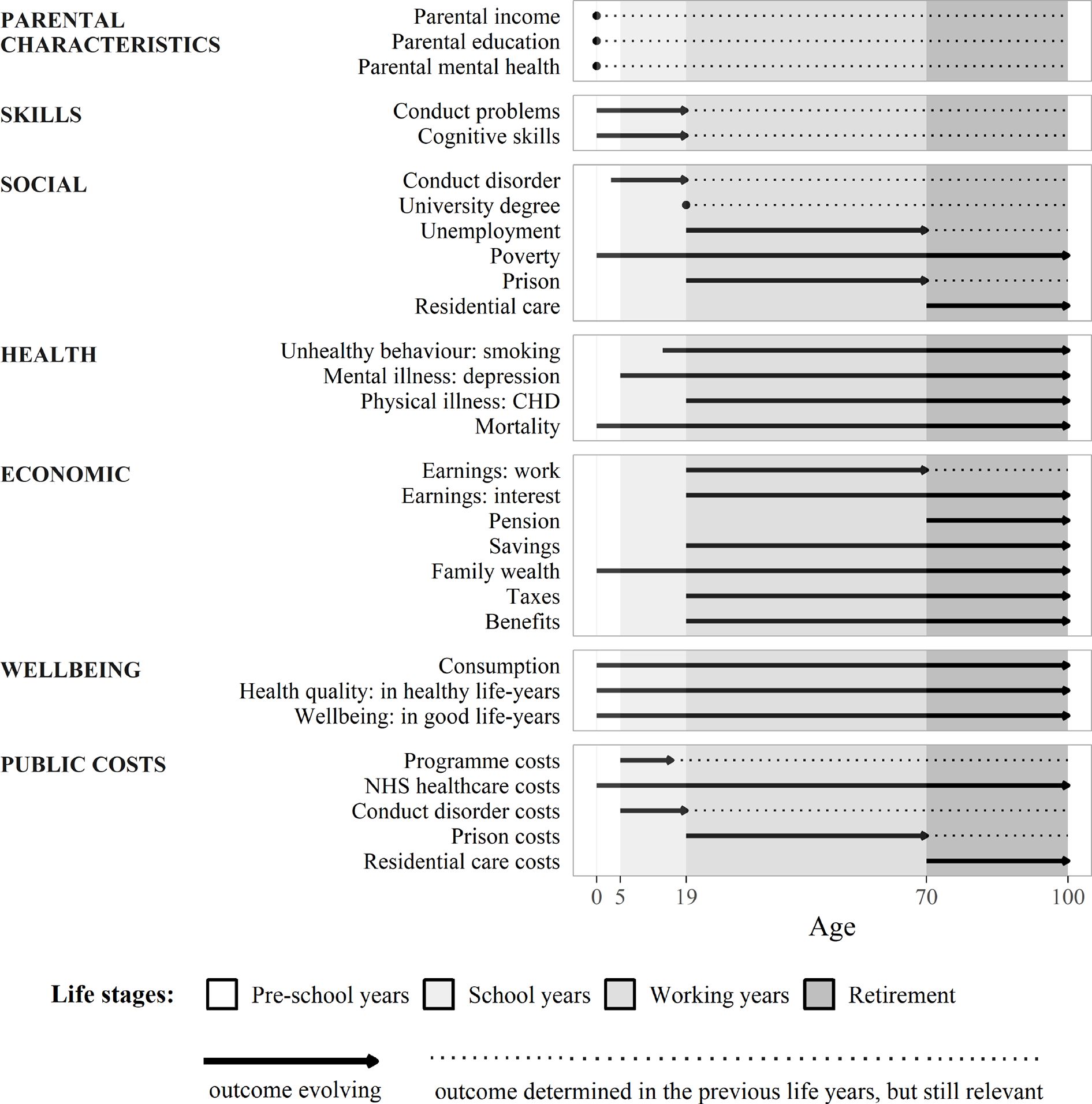
Overview of Key Outcomes Over the Lifecourse
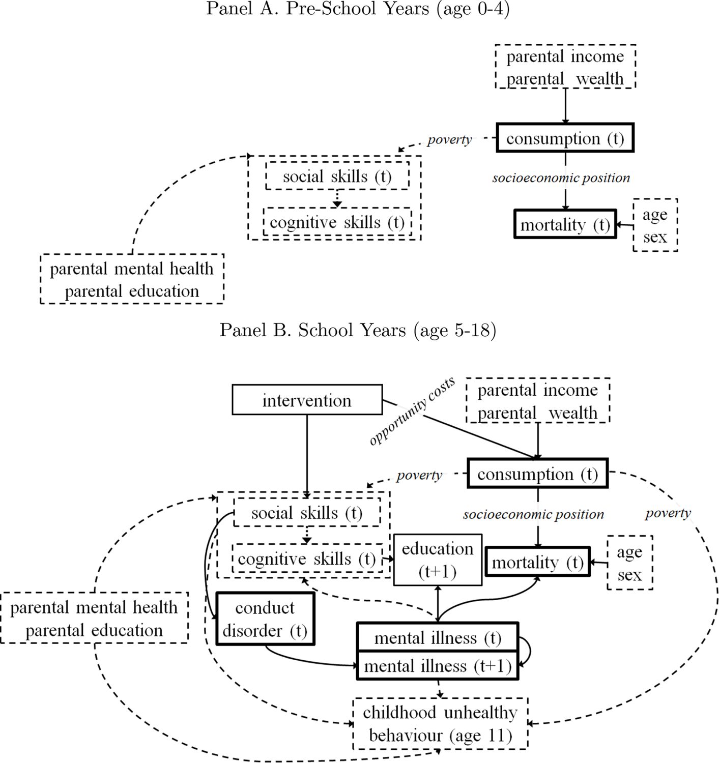
Model Structure for Key Life Stages in Childhood

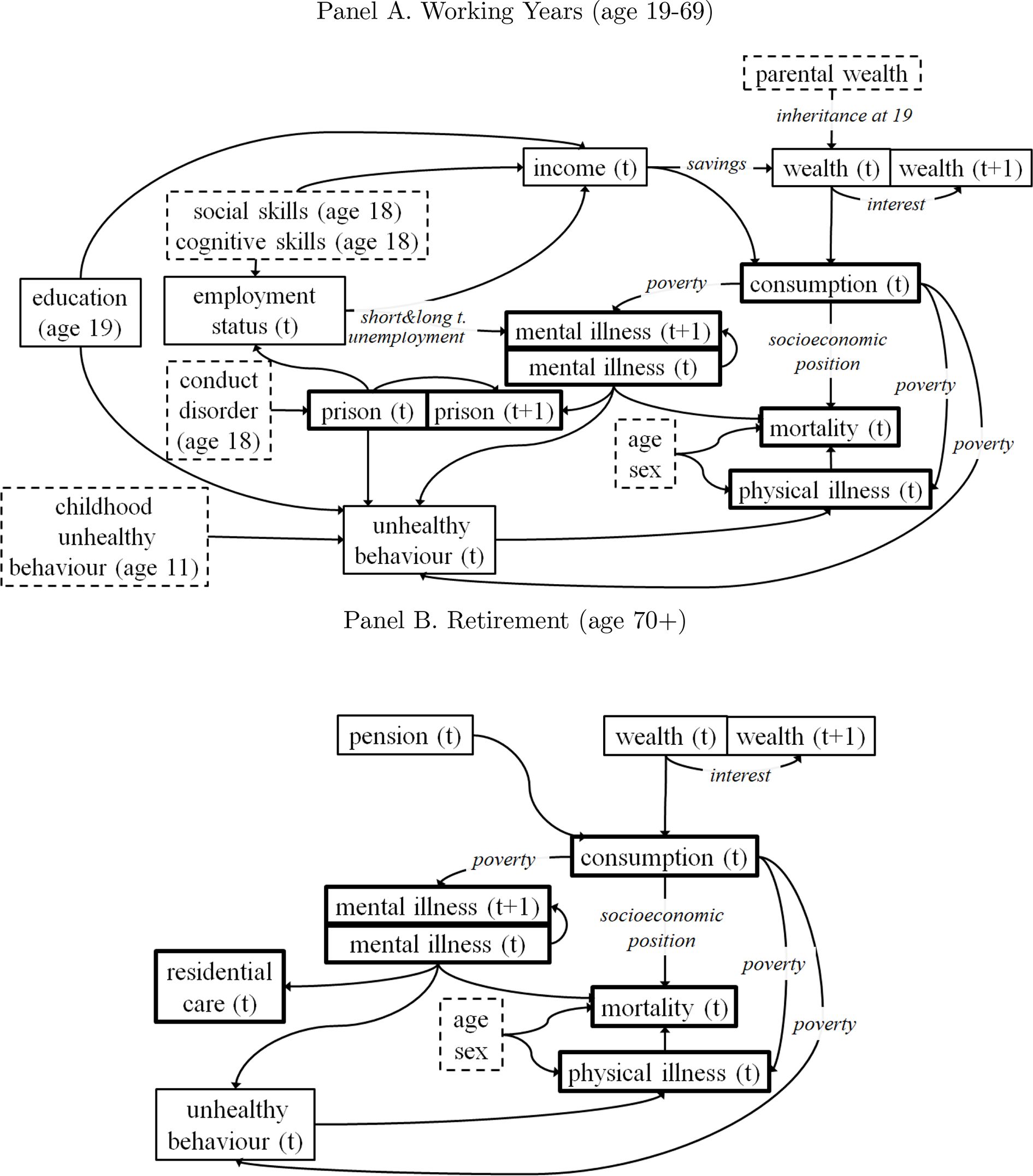
Model Structure for Key Life Stages in Adulthood

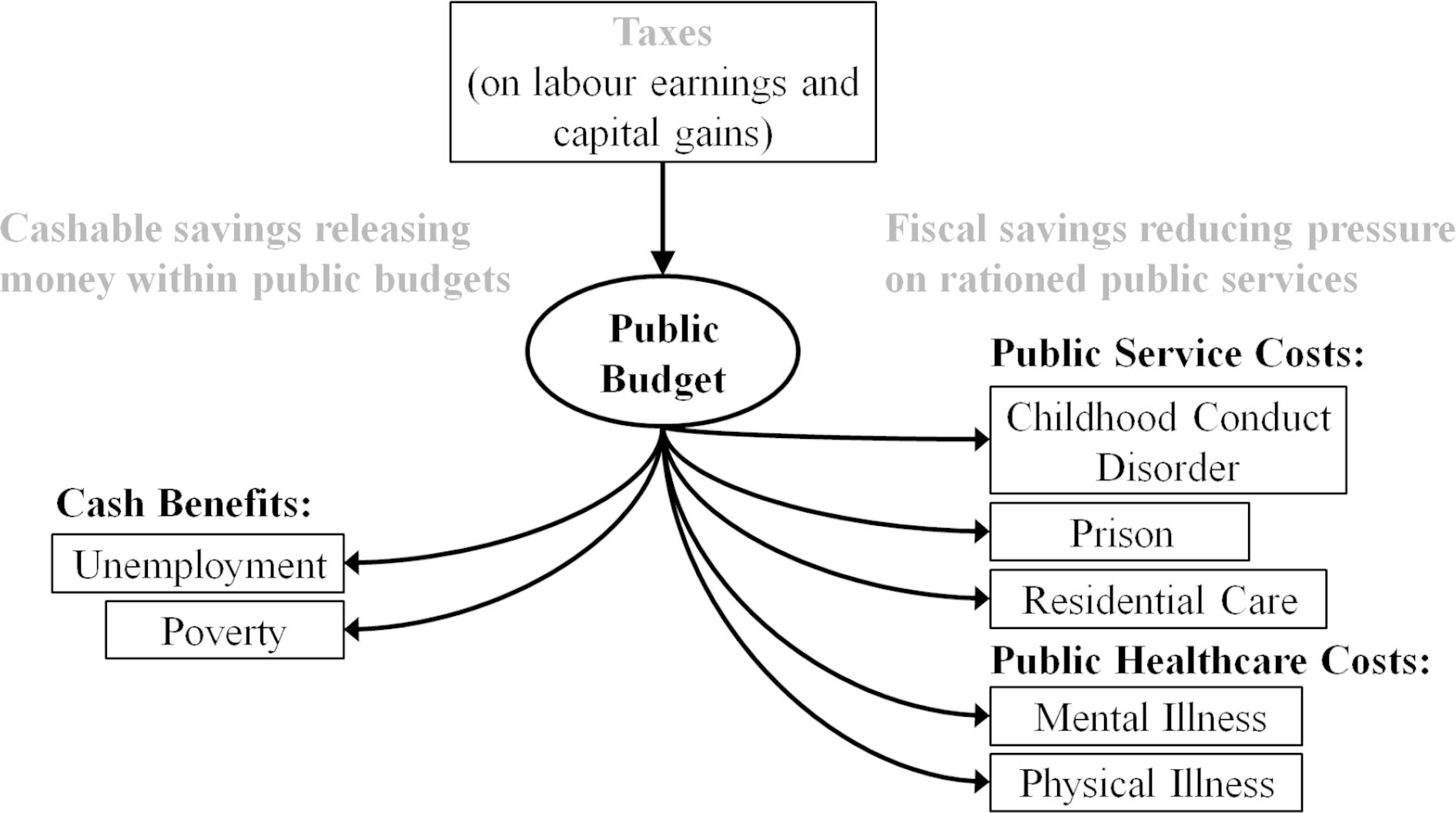
Model Structure for Public Costs

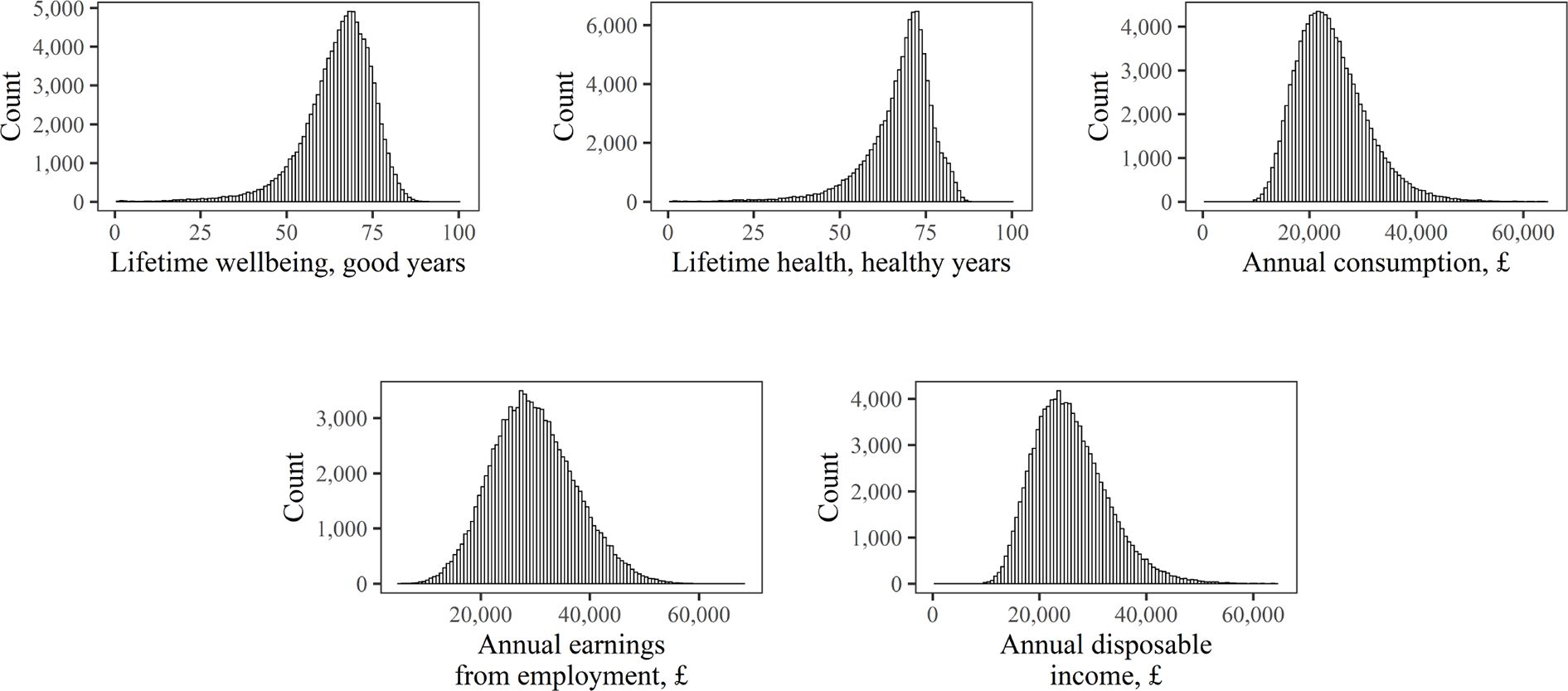
Distributions of Core Outcomes

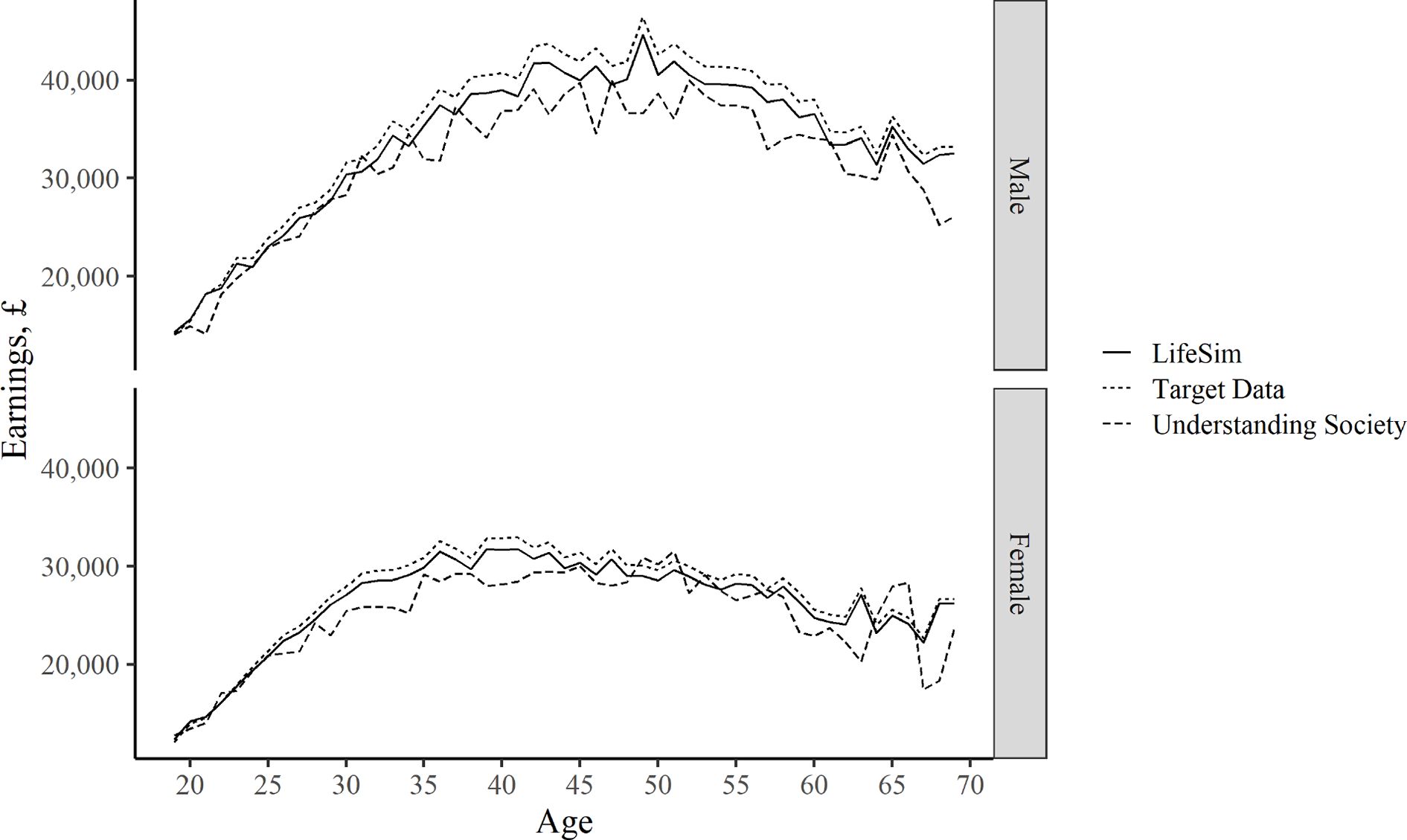
Earnings: Comparison with Other Data Sources

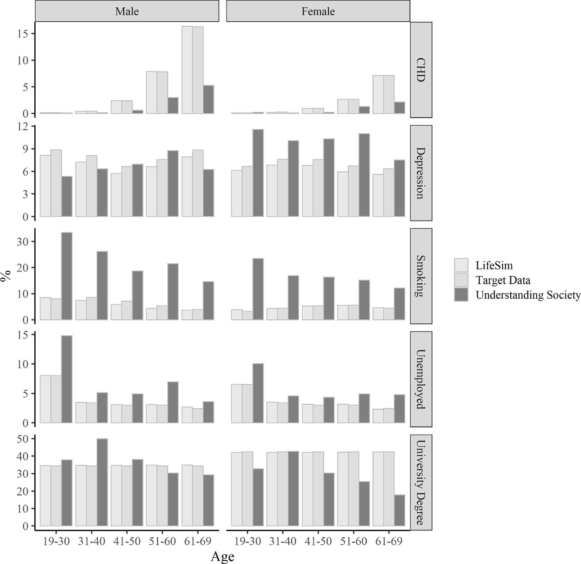
Other Outcomes: Comparison with Understanding Society

Earnings: Comparison with Other Data Sources
Tables
Summary of Child Characteristics and Family Conditions
| Child's characteristic / family condition | Data used in modelling | Source | Mean | SD | Min | Max |
|---|---|---|---|---|---|---|
| A: BASIC CHILD’S CHARACTERISTICS | ||||||
| Sex | Indicator if child is male | MCS1 | 0.49 | 0.50 | 0 | 1 |
| Teenage smoking | Indicator if child smokes at 14 | MCS6 | 0.16 | 0.37 | 0 | 1 |
| B: SOCIAL CONDITIONS | ||||||
| Parental income | OECD equivalised household income after taxes and benefits, £ | MCS1 | 32,004 | 19,972 | 1,445 | 128,246 |
| Parental wealth | Parental assets, £ | MCS5 | 3,068 | 19,937 | 0 | 600,000 |
| Parental socio-economic position | Household income quintile | MCS1 | 3.06 | 1.37 | 1 | 5 |
| Childhood poverty | Indicator if household income is below 60% median | MCS1 | 0.27 | 0.45 | 0 | 1 |
| C: PARENTAL CHARACTERISTICS | ||||||
| Parental education | Indicator if parent has a university degree (NVQ 4 or above) | MCS1 | 0.31 | 0.46 | 0 | 1 |
| Parental depression at child’s birth | Indicator if Rutter malaise inventory score is 4 or above | MCS1 | 0.14 | 0.35 | 0 | 1 |
| Parental depression severity at child’s birth | 9-item Rutter malaise inventory score | MCS1 | 1.66 | 1.68 | 0 | 9 |
| Parental depression when child is 5 years old | Indicator if Kessler psychological distress scale score is 13 or above | MCS3 | 0.03 | 0.18 | 0 | 1 |
| Parental depression severity when child is 5 years old | 6-item Kessler psychological distress scale score | MCS3 | 3.17 | 3.72 | 0 | 24 |
| D: CHILD’S SOCIAL SKILLS | ||||||
| Conduct problems up to age 4 | SDQ conduct problem score (see the note) | MCS2 | 2.87 | 2.02 | 0 | 10 |
| Conduct problems, ages 5-6 | SDQ conduct problem score | MCS3 | 1.46 | 1.47 | 0 | 8 |
| Conduct problems, ages 7-10 | SDQ conduct problem score | MCS4 | 1.32 | 1.50 | 0 | 9 |
| Conduct problems, ages 11-13 | SDQ conduct problem score | MCS5 | 1.38 | 1.58 | 0 | 10 |
| Conduct problems, age 14+ | SDQ conduct problem score | MCS6 | 1.42 | 1.68 | 0 | 10 |
| Impact of problems up to age 4 | SDQ impact supplement score | MCS2 | 0.11 | 0.58 | 0 | 8 |
| Impact of problems, ages 5-6 | SDQ impact supplement score | MCS3 | 0.13 | 0.63 | 0 | 8 |
| Impact of problems, age 7+ | SDQ impact supplement score | MCS4 | 0.25 | 0.91 | 0 | 9 |
| E: CHILD’S COGNITIVE SKILLS | ||||||
| Cognitive skills up to age 4 | Various measures (see the note) | MCS2 | 1.02 | 0.14 | 0.58 | 1.44 |
| Cognitive skills, ages 5-6 | Various measures | MCS3 | 1.03 | 0.13 | 0.57 | 1.45 |
| Cognitive skills, ages 7-10 | Various measures | MCS4 | 1.03 | 0.14 | 0.56 | 1.41 |
| Cognitive skills, ages 11-13 | Various measures | MCS5 | 1.03 | 0.15 | 0.39 | 1.49 |
| Cognitive skills, age 14+ | Various measures | MCS6 | 1.02 | 0.14 | 0.43 | 1.50 |
-
Note: The analysis is for 100,000 individuals in the LifeSim cohort. MCS denotes MCS sweep j (6 sweeps in total). Children were 9 months old in MCS1, 3 years old in MCS2, 5 years old in MCS3, 7 years old in MCS4, 11 years old in MCS5 and 14 years old in MCS6. SDQ conduct problem and impacts scores have a scale 0-10, with a higher value representing more problems/higher impact of problems. The cognitive skills measure is an age-specific common factor extracted from the various cognitive skills measures in MCS, including the British Ability Scales II, Bracken School Readiness Assessment, National Foundation for Educational Research Progress in Maths, Cambridge Neuropsychological Test Automated Battery tests and Applied Psychology Unit.
Determinants of the Modelled Outcomes
| Outcomes (Y) | Determinants (X) | |||
|---|---|---|---|---|
| Name | Type | Other modelled outcomes (parameter source in brackets) | Exogenous variables | |
| From childhood dataset (MCS) | From target datasets | |||
| SOCIAL | ||||
| Conduct disorder | P, I | SDQ conduct problem score, SDQ impact score (both Goodman et al. (2015)); | ||
| Education (university degree) | P, I | Poverty at age 18 (Goodman et al., 2015; Fletcher, 2010; Farahati et al., 2003); | Cognitive skills (age 14), SDQ conduct problem score (age 14) (both Goodman et al. (2015)); | Estimated likelihood of a person participating in Higher Education by age 30 (DE, 2016); |
| Unemployment (employment) | P, I | L.prob. of employment; prison; age; | Cognitive skills (age 14) (Goodman et al. (2015)), SDQ conduct problem score (age 14) (both Goodman et al. (2015)); | Employment rate in UK by age and sex (ONS, 2018); |
| Poverty | I | Consumption; | 60% equivalised household income in UK (ONS, 2011); | |
| Prison | P, I | L.prob. of prison; conduct disorder at age 18 (Fergusson et al., 2005); L.depression (Anderson et al., 2015); | Prison rates in England by age and sex ( MJ, 2017 and ONS, 2018); | |
| Residential care | P, I | L.prob. of residential care; L.depression (McDougall et al., 2007; Stewart et al., 2014); | Rates of people aged 65+ in care home by sex in England (ONS, 2011). | |
| HEALTH | ||||
| Smoking | P, I | L.prob. of smoking; education, poverty (both Jefferis et al. (2003)); depression (Lasser et al., 2000), prison (Singleton et al., 2003); | Teenage smoking rates by sex (MCS, age 14) (param. from Jefferis et al. (2003)), smoking rate in England by age, sex and IMD quintile group (HSE, 2006); | |
| Coronary heart disease (CHD) | P, I | L.prob. of CHD; L.smoking (Bazzano et al., 2003; Critchley and Capewell, 2003); L.poverty (Marmot et al., 1997); | CHD rates in England by age, sex and IMD quintile group (HSE, 2006); | |
| Depression | P, I | L.prob. of depression; L.conduct disorder (Luby et al., 2014); employment (Thomas et al., 2005); poverty (Weich and Lewis, 1998); | Emotional disorder rates in England by age, sex and IMD quintile group (MHCYPGB, 2004), depression rates in England by age, sex and IMD quintile group (HSE, 2014); | |
| Mortality | P, I | Depression (Chang et al., 2010); CHD (estimated using HSE (2006) and ONS data); | Mortality rates in England by age, sex and IMD quintile group (ONS, 2011); | |
| ECONOMIC | ||||
| Earnings from employment (gross), £ | C | Education (Blundell et al., 2000) ; employment; age; | Cognitive skills at age 14, SDQ conduct problem score at age 14 (both Goodman et al. (2015)); | Full time annual gross pay in UK by age and sex (ONS, 2015); |
| Interest, £ | C | L.Wealth; | Interest rates in UK; | |
| Pension, £ | C | Years in employment; age; | Level of state pension in UK; | |
| Savings, £ | C | Earnings from employment; interest; taxes; L.consumption; | ||
| Wealth, £ | C | L.Wealth; Earnings from employment; interest; pension; tax; consumption; residential care; age; | Parental wealth; parental income; | |
| Taxes, £ | C | Earnings from employment; interest; pension; | Income tax brackets in UK; | |
| Benefits, £ | C | Earnings from employment; interest; pension; wealth; residential care; | Parental income; | Conditions for claiming benefits in UK; |
| WELLBEING | ||||
| Consumption, £ | C | Earnings from employment; interest, pension; taxes; savings; residential care; L.consumption, L.wealth; | Parental income; | |
| Health quality, QALYs | C | CHD, depression (both Sullivan et al. (2011)); | Average health quality in England by age, sex and IMD quintile group (Love-Koh et al., 2015); | |
| Wellbeing, wellbeing-QALYs | C | Health quality, consumption (both Cookson et al. (2021)). | ||
-
Note: Outcome types: P -- probability, I -- indicator, C -- continuous. Other abbreviations: prob. - probability, L. -- lagged (previous year), MCS -- Millennium Cohort Study, ONS -- Office for National Statistics, HSE -- Health Survey for England, MHCYPGB -- Mental Health of Children and Young People in Great Britain, IMD -- Index of Multiple Deprivation, DE -- Department of Education. Full references for the parameter sources are in the Appendix B.
Summary Statistics of the Simulated Outcomes
| Outcome | Baseline simulation | Bootstrap simulation | ||||
|---|---|---|---|---|---|---|
| Mean | SD | Min | Max | Mean | SE | |
| CHILD OUTCOMES | ||||||
| Conduct disorder at age 5, % | 8.63 | 28.08 | 0.00 | 100.00 | 8.59 | 0.10 |
| Conduct disorder at age 18, % | 9.09 | 28.74 | 0.00 | 100.00 | 9.00 | 0.08 |
| ADULT OUTCOMES | ||||||
| Proportion of university graduates, % | 38.51 | 48.66 | 0.00 | 100.00 | 38.51 | 0.15 |
| Proportion of working years in unemployment, % | 5.73 | 6.63 | 0.00 | 100.00 | 5.70 | 0.02 |
| Proportion of lifetime in poverty, % | 26.85 | 18.30 | 0.00 | 100.00 | 26.80 | 0.05 |
| Proportion of working years in prison, % | 1.62 | 5.12 | 0.00 | 75.00 | 1.60 | 0.01 |
| Proportion of retirement in residential care, % | 1.28 | 3.95 | 0.00 | 100.00 | 1.28 | 0.02 |
| Proportion of adult years as a smoker, % | 5.32 | 5.12 | 0.00 | 100.00 | 5.31 | 0.02 |
| Proportion of adult years with CHD, % | 6.16 | 4.07 | 0.00 | 33.33 | 6.15 | 0.01 |
| Proportion of life years with mental illness, % | 5.98 | 2.81 | 0.00 | 25.81 | 5.99 | 0.01 |
| Years of life | 78.78 | 13.04 | 0.00 | 100.00 | 78.80 | 0.04 |
| Premature mortality rate (before age 75), % | 28.13 | 44.96 | 28.04 | 0.14 | ||
| Annual earnings (lifetime average), £ | 29,655 | 7,638 | 4,792 | 67,879 | 29,659 | 23 |
| Annual savings (lifetime average), £ | 2,833 | 942 | 0 | 7,803 | 2,832 | 3 |
| Annual interest (lifetime average), £ | 402 | 234 | 0 | 3,321 | 402 | 1 |
| FINAL WELLBEING OUTCOMES | ||||||
| Annual consumption (lifetime average), £ | 24,114 | 6,648 | 10,000 | 113,817 | 24,115 | 22 |
| Healthy years | 68.28 | 9.99 | 0.87 | 88.16 | 68.30 | 0.03 |
| Healthy years (discounted) | 40.94 | 3.96 | 0.87 | 48.01 | 40.96 | 0.01 |
| Good years | 65.67 | 10.21 | 0.69 | 91.93 | 65.69 | 0.03 |
| Good years (discounted) | 39.80 | 4.89 | 0.69 | 52.18 | 39.82 | 0.01 |
-
Note: The baseline simulation mean, standard deviation (SD), minimum value (Min) and maximum value (Max) are calculated for the simulated population of 100,000 (for the lifetime aggregates, or yearly – for the annual variables). The bootstrap simulation mean and standard error (SE) are calculated for the distribution of the means of the 100 bootstrap simulations. The time periods for calculating life-stage proportions are as follows: ‘working years’ refer to the period between ages 19-69; ‘retirement’ refers to the time period from age 70 up to death; adult years refer to the time period from age 19 up to death; lifetime refers to the entire period from birth to death. CHD – coronary heart disease. We use year 2015/16 prices and the annual discount rate of 1.5% (Paulden and Claxton, 2012).
Cumulative Costs Over Various Time Periods
| Costs (Per Capita), £ | Age 0-10 | Age 0-15 | Age 0-20 | Age 0-25 | Lifetime |
|---|---|---|---|---|---|
| GENERAL POPULATION COHORT | |||||
| PUBLIC SERVICES | |||||
| Conduct disorderPrisonResidential care | 1,10000 | 1,70000 | 1,8009300 | 1,8003,2000 | 1,80017,0001,200 |
| HEALTHCARE | |||||
| CHDDepressionOther | 07409,300 | 01,90014,000 | 03,60020,000 | 04,90027,000 | 1,40014,00088,000 |
| Benefit payments | 1,400 | 2,100 | 4,100 | 6,300 | 12,000 |
| LOWEST INCOME QUINTILE GROUP AT BIRTH | |||||
| PUBLIC SERVICES | |||||
| Conduct disorderPrisonResidential care | 1,40000 | 2,10000 | 2,2001,1000 | 2,2004,0000 | 2,20020,0001,200 |
| HEALTHCARE | |||||
| CHDDepressionOther | 077011,000 | 02,00016,000 | 03,60022,000 | 05,00029,000 | 1,40014,00091,000 |
| Benefit payments | 8,600 | 12,000 | 17,000 | 19,000 | 22,000 |
| TOP INCOME QUINTILE GROUP AT BIRTH | |||||
| PUBLIC SERVICES | |||||
| Conduct disorderPrisonResidential care | 88000 | 1,30000 | 1,5008000 | 1,5002,7000 | 1,50014,0001,100 |
| HEALTHCARE | |||||
| CHDDepressionOther | 07108,400 | 01,90013,000 | 03,50018,000 | 04,90025,000 | 1,40014,00085,000 |
| Benefit payments | 0 | 0 | 1,300 | 3,000 | 7,900 |
-
Note: All values are calculated per simulated individual in year 2015/16 prices, and discounted at 1.5% annual rate, and rounded to 2 significant figures. See details on cost sources in Table A6 in Appendix A.
Whole Cohort Lifetime Inequality by Childhood Circumstance
| Childhood circumstance | Number of children | Annual consumption, £ | Lifetime health, healthy years | Lifetime wellbeing, good years |
|---|---|---|---|---|
| Best off 20% | 20,000 | 32,559 | 68.71 | 69.59 |
| Worst off 20% | 20,000 | 18,471 | 66.31 | 59.84 |
| Difference | 14,088 | 2.407 | 9.76 | |
| Extreme best off 20% | 12,149 | 32,909 | 68.81 | 69.83 |
| Extreme worst off 20% | 26 | 16,808 | 62.16 | 54.51 |
| Difference | 16,101 | 6.66 | 15.32 |
-
Note: The average policy gains per cohort member for the subgroups of the simulated cohort of 100,000 individuals.
Comparison with the British Cohort 1970
| Outcome | N | Mean | Differencein means | SD | Difference | |||
|---|---|---|---|---|---|---|---|---|
| LifeSim | BCS70 | LifeSim | BCS70 | LifeSim | BCS70 | in SDs | ||
| AGE 26 | ||||||||
| Male (indicator) | 99,402 | 9,003 | 0.48 | 0.46 | 0.03 | 0.50 | 0.50 | 0.00 |
| University Degree (indicator) | 99,402 | 8,399 | 0.39 | 0.25 | 0.13 | 0.49 | 0.43 | 0.05 |
| Employed (indicator) | 99402 | 9003 | 0.95 | 0.96 | -0.01 | 0.23 | 0.20 | 0.02 |
| Earnings (in year 2015 £) | 99,402 | 6,642 | 19,736 | 14,279 | 5,457 | 5,882 | 7,110 | -1,228 |
| Depression (indicator) | 99402 | 9003 | 0.07 | 0.10 | -0.03 | 0.25 | 0.30 | -0.05 |
| Smoking (indicator) | 99,402 | 8,892 | 0.06 | 0.27 | -0.20 | 0.25 | 0.44 | -0.20 |
| AGE 29 | ||||||||
| Male (indicator) | 99,267 | 11,261 | 0.48 | 0.49 | -0.00 | 0.50 | 0.50 | -0.00 |
| University Degree (indicator) | 99,267 | 11,211 | 0.39 | 0.27 | 0.11 | 0.49 | 0.44 | 0.04 |
| Employed (indicator) | 99,267 | 9,506 | 0.94 | 0.96 | -0.02 | 0.23 | 0.19 | 0.04 |
| Earnings (in year 2015 £) | 99,267 | 8,102 | 22,400 | 20,796 | 1,604 | 6,682 | 68,798 | -62,115 |
| Depression (indicator) | 99,267 | 11,261 | 0.07 | 0.10 | -0.03 | 0.25 | 0.30 | -0.05 |
| Smoking (indicator) | 99,267 | 11,205 | 0.06 | 0.29 | -0.23 | 0.24 | 0.45 | -0.22 |
| AGE 42 | ||||||||
| Male (indicator) | 98,149 | 9,841 | 0.48 | 0.48 | 0.00 | 0.50 | 0.50 | 0.00 |
| University Degree (indicator) | 98,149 | 9,841 | 0.39 | 0.34 | 0.05 | 0.49 | 0.47 | 0.01 |
| Employed (indicator) | 98,149 | 8,594 | 0.95 | 0.97 | -0.02 | 0.21 | 0.16 | 0.05 |
| Earnings (in year 2015 £) | 98,149 | 2,158 | 29,327 | 22,107 | 7,220 | 9,604 | 15,567 | -5,963 |
| Depression (indicator) | 98,149 | 9,756 | 0.07 | 0.11 | -0.04 | 0.26 | 0.31 | -0.05 |
| Smoking (indicator) | 98,149 | 9,801 | 0.06 | 0.20 | -0.14 | 0.24 | 0.40 | -0.17 |
| AGE 46 | ||||||||
| Male (indicator) | 97,532 | 8,581 | 0.48 | 0.48 | -0.00 | 0.50 | 0.50 | -0.00 |
| University Degree (indicator) | 97,532 | 8,444 | 0.39 | 0.34 | 0.04 | 0.49 | 0.47 | 0.01 |
| Employed (indicator) | 97,532 | 5,038 | 0.95 | 0.99 | -0.03 | 0.21 | 0.12 | 0.09 |
| Earnings (in year 2015 £) | 97,532 | 358 | 28,558 | 22,538 | 6,020 | 9,978 | 31,559 | -21,581 |
| CHD (indicator) | 97,532 | 8,353 | 0.02 | 0.00 | 0.02 | 0.15 | 0.05 | 0.10 |
| Depression (indicator) | 97,532 | 8,486 | 0.06 | 0.14 | -0.08 | 0.23 | 0.35 | -0.12 |
| Smoking (indicator) | 97,532 | 8,578 | 0.05 | 0.15 | -0.10 | 0.23 | 0.36 | -0.13 |
-
Note: N – number of observations, SD – standard-deviation. We quantify the difference between the LifeSim distribution and BCS70 distribution in terms of the absolute difference in their means and standard deviations. Earnings is the net pay from employment.
Notation
| Notation | Explanation |
|---|---|
| SIMULATED VARIABLES | |
| Recipient for the parent-training programme (indicator); | |
| Conduct problem measure; | |
| Impact of problems; | |
| Childhood conduct disorder (indicator); | |
| Cognitive skills; | |
| University degree (indicator); | |
| Smokes (indicator); | |
| Mental illness (indicator); | |
| Coronary heart disease (CHD) (indicator); | |
| Dead (indicator); | |
| In prison (indicator); | |
| In residential care (indicator); | |
| Employed (indicator); | |
| Annual earnings, £; | |
| Lifetime accumulated wealth; | |
| Annual consumption level, £; | |
| In poverty (indicator); | |
| Annual amount of taxes paid; | |
| Annual amount of benefits received; | |
| Savings rate; | |
| Minimum consumption level, which government subsidises if it cannot be sustained by an individual; | |
| Male (indicator); | |
| Socio-economic position (quintile group); | |
| SDQ conduct problem score reported in MCS sweep j (j = 2; 3; 4; 5; 6); | |
| SDQ impact score reported in MCS sweepj; | |
| Extracted factor using principal component analysis based on cognitive skills tests reported in MCS sweep j, standardised with a mean of 1.00 and standard deviation of 0.15 following Jones and Schoon (2008); | |
| OTHER NOTATION | |
| prefix pr. | Probability, i.e. denotes probability of smoking; |
| line over variable (—) | Mean calculated from a target dataset, i.e. is proportion of people smoking in a particular age and sex group; |
| prefix trend. | Modelled time trend, i.e. the mean increase in variable over time, estimated from a target dataset, i.e. during working years expected earnings increase as people get past their youth, as they gain work experience, climb the career ladder, etc.; |
| prefix sd. | Modelled variation in some variable, i.e. standard deviation in the variable, estimated from a target dataset; |
| Parameter representing the effect of some outcome denotes the effect of smoking on CHD risk. Depending on the context, we use it to represent coefficients from a linear regression, odds-ratios, etc. See full list of parameters, and their sources in Table A3; | |
| Standard mortality ratio given condition x, i.e. the probability of dying from condition x divided by the probability of dying in the general population. |
-
Note: MCS – Millennium Cohort Study.
Target Data
| Parameter | Description | Source |
|---|---|---|
| Mortality rates (by age, sex and the English IMD quintile group); | ONS, 2011; | |
| Ages 5-18: proportion of children with any emotional disorder (by age, sex, and IMD quintile group); age 18+: depression diagnosed by a doctor and present or being treated within the past 12 months in England (by age, sex, and English IMD quintile group); | For age 5-18: Mental Health of Children and Young People Great Britain, 2004; age 18+: Health Survey for England, 2014; | |
| Proportion of people with CHD in England (by age, sex, and English IMD quintile group); | Health Survey for England, 2006; | |
| Mean full time annual gross pay in UK (by age and sex); | Annual Survey of Hours and Earnings, ONS, 2015; | |
| Seasonally adjusted employment rate, expressed as a proportion of the economically active population (by age and sex); | Labour Force Survey, ONS, 2018; | |
| Mean SDQ conduct problem score (by age and sex); | MCS, 2000–2014; | |
| Mean cognitive measure (by age and sex); | MCS, 2000–2014; | |
| Higher Education Initial Participation Rate in 2015/2016 (estimate of the likelihood of a person participating in Higher Education by age 30, based on current participation rates, adjusted by the probability of dropping out); | Department for Education, 2016; | |
| Proportion of 14-year-old children smoking (by sex); | MCS, 2014; | |
| Proportion of daily smokers in England (by age, sex and English IMD quintile group) in England; | Health Survey for England, 2006; | |
| Proportion of households below 60% median income by sex in UK; | Family Resources Survey, Department for Work & Pensions, 2016/2017; | |
| Proportion of 4-year-old children with conduct disorder (by age, sex); | Mental Health of Children and Young People Great Britain, 2004; | |
| Average proportion of people in prison (by age and sex) in England and Wales over 31 March 2017 - 31 March 2018 (calculated using population estimates in mid-2017); | Offender Management Statistics, Ministry of Justice, 2017-2018; Population Estimates for UK, England and Wales, Scotland and Northern Ireland Mid-2017, ONS; | |
| Proportion of people aged 65+ in resident care homes (by sex) in England and Wales, 2011; | “Changes in the older resident care home population between 2001 and 2011” 2014, ONS. |
-
Note: MCS – Millennium Cohort Study, ONS – Office for National Statistics, IMD – Index of Multiple Deprivation. Our notation uses an overline to denote averages from a target dataset.
Parameters
| Parameter | Value | Source | Notes |
|---|---|---|---|
| 3.21 among 15-44 year olds, 1.75 – 45-64 year olds and 1.18 for 65+ | Chang et al. (2010) | Age standardised mortality ratios in southeast London 2007–2009, for people with depressive episode against the general population of England and Wales in 2008; | |
| See Table A5 | Health survey for England (2006); the 20th Century Mortality Files, ONS; Mid-year population estimates for England and Wales, ONS | Estimated probability of dying from CHD among those who have a CHD, in England and Wales, 2008 using CHD prevalence rates of 2006; | |
| ln 1.004/SDsdq.cp | Goodman et al. (2015) social | 0.4% increase in gross wage with standard deviation increase in externalising subscale (conduct+peer); SDs dq.cp – standard deviation of SDQ conduct problem score in the relevant age-sex subgroup of our simulation. | |
| ln 1.072/SDcog | Goodman et al. (2015) social | 7.2% increase in gross wage with standard deviation increase in IQ score; SDcog – standard deviation of cognitive skills in the relevant age-sex subgroup of our simulation. | |
| ln 1.17if male; ln 1.37if female | Blundell et al. (2000) | 17% increase in hourly wage from having undergraduate degree for males, 37% for females; | |
| Goodman et al. (2015) social | standard deviation increase in cognitive ability associated with 12% point increase in prob. obtaining a degree; | ||
| Goodman et al. (2015) social | standard deviation decrease in Rutter externalising score associated with 2.2% point increase in prob. obtaining a degree; | ||
| -0.04 | Goodman et al. (2015) social; Fletcher (2010) adolescent; Farahati et al. (2003) effects | goodman2015social fletcher2010adolescent find no statistically significant effect; but fletcher2010adolescent finds that being depressed increases the probability of dropping out of high school by around 2.4% points, and decreases the probability of college enrolment by 2.7–7.2 percentage points. farahati2003effects find that parent’s depression increases child’s probability of dropout by over 3% points for females. In the light of these findings, the current model specification sets the parameter at 4% points; | |
| ln 3.38 if male; ln 3.68 if female | Jefferis et al. (2003) cigarette | Estimates obtained using logistic regression; | |
| ln 1.91 if male; ln 1.81if female | Jefferis et al. (2003) cigarette | Estimates obtained using logistic regression; | |
| ln 3.32if male; ln 3.26if female | Jefferis et al. (2003) cigarette | Estimates obtained using logistic regression; | |
| ln 2.7 | Lasser et al. (2000) smoking | Estimates obtained using logistic regression; | |
| 0.07 if male and 0.06 if female | Singleton et al. (2003) substance | Calculated using the prevalence rates in a population before and after imprisonment, does not take into account the contribution of this increase because of mental illness, poverty and potentially other variables; | |
| ln 3.63 | Luby et al. (2014) trajectories | Including the effect that occurs via non-supportive parenting (see discussion below); estimated using logistic regression; | |
| ln 2.05 if male;ln 1.72if female | Thomas et al. (2005) employment | Estimated using logistic regression; the effect on psychological problems measured by general health questionnaire; | |
| ln 0.87 if male; ln 0.79 if female | Thomas et al. (2005) employment | Estimated using logistic regression; the effect on psychological problems measured by general health questionnaire; | |
| ln 1.24 | Weich and Lewis (1998) material | Estimated using logistic regression; the effect on psychological problems measured by general health questionnaire; | |
| ln 1.49 if male; ln 1.18if female | Marmot et al. (1997) contribution | Calculated using logistic regression controlling for age and CHD risk factors (incl. smoking), social support and job control. Using the parameters depends on assuming poverty correlates with low employment grade; | |
| ln 2 | Bazzano et al. (2003) relationship, Critchley and Capewell (2003) mortality | Based on estimates of odds ratios reported in the cited sources (see discussion in section A.1.2); | |
| 0.18 | Fergusson et al. (2005) show | Estimated using rates of arrests/convictions among people with different levels of conduct problems; | |
| 0.015 | Anderson et al. (2015) youth | ||
| 0.18 | McDougall et al. (2007) prevalence; Stewart et al. (2014) current | Calculated using depression prevalence rates; | |
| Goodman et al. (2015) social | Standard deviation increase in externalising subscale of SDQ raises probability being employed by 1.6%; SD sdq.cp – standard deviation of SDQ conduct problem score in the relevant age-sex subgroup of our simulation; | ||
| Goodman et al. (2015) social | Standard deviation increase in IQ test score raises probability being employed by 2.1%;SDcog – standard deviation of the cognitive skills measure in the relevant age-sex subgroup of our simulation. |
Modelled Variables and Controls
| Y | Effect parameter | Method | Parameter reported | Explanatory variables (X) in the modelling equation | ||||||||||||||
|---|---|---|---|---|---|---|---|---|---|---|---|---|---|---|---|---|---|---|
| Cond. prob. | CD | Cog. skills | Education | Smoking | Teen. smoking | Depression | CHD | Employment | Prison | Res. care | Poverty | Income | Age | Sex | ||||
| SOCIAL | ||||||||||||||||||
| Education | ||||||||||||||||||
| Conduct problems | Probit; | AME; | √ | √ | ✵ | (√) | (√) | (√) | ||||||||||
| Cognitive skills | Probit; | AME; | √ | √ | ✵ | (√) | (√) | (√) | ||||||||||
| Depression | Probit; | AME; | ✵ | √ | √ | (√) | (√) | (√) | (√) | |||||||||
| Unemployment | Conduct problems | Probit; | AME; | √ | √ | ✵ | (√) | (√) | (√) | |||||||||
| Cognitive skills | Probit; | AME; | √ | √ | ✵ | (√) | (√) | (√) | ||||||||||
| Prison | CD | Compare prevalence rates across subgroups, test the significance of relationships using logit; | Average rates of being arrested/convicted among the different subgroups; | (√) | √ | (√) | ✵ | (√) | (√) | |||||||||
| Depression | OLS (robustness checks with probit and logit yield similar results); | Regression coefficient; | √(control for drug, alcohol and marijuana use, ADHD, bad temper and anxiety during adolescence) | (√) | (√) | √ | (√) | (√) | (√) | (√) | (√) | |||||||
| Residential care | Depression | Compare prevalence rates across subgroups; | Age and sex adjusted difference between subgroups; | √ | (√) | (√) | ||||||||||||
| HEALTH | ||||||||||||||||||
| Smoking | Education | Logit; | OR; | √ | √ | ✵ | ✵ | ✵ | (√) | |||||||||
| Teenage smoking | Logit; | OR; | ✵ | √ | ✵ | ✵ | √(manual social class) | (√) | ||||||||||
| Poverty | Logit; | OR; | ✵ | √ | ✵ | ✵ | √ | (√) | ||||||||||
| Depression | Logit; | OR; | ✵ | ✵ | √ | ✵ | ✵ | (√) | (√) | |||||||||
| Prison | Comparison of smoking status pre and post imprisonment; | Increase in smoking rate post imprisonment; | ✵ | ✵ | ✵ | √ | ✵ | (√) | ||||||||||
| Depressed | CD | Logit; | OR; | √ | √(family income-to-needs ratio) | (√) | ||||||||||||
| Unemployment | Logit; | OR; | ✵ | √(prior mental illness) | √ | ✵ | (√) | (√) | ||||||||||
| Poverty | Logit; | OR; | ✵ | (√) | √ | √ | (√) | (√) | (√) | |||||||||
| CHD | Smoking | Logit; | OR; | √ | ✵ | (√) | (√) | |||||||||||
| Poverty | Logit; | OR; | √ | √(low employment grade) | (√) | (√) | ||||||||||||
| Mortality | Depression | Estimation of standardised mortality ratios; | Age standardised mortality ratio; | √ | ✵ | (√) | (√) | |||||||||||
| CHD | Estimation of dying probability from CHD; | Probability of dying from CHD; | ✵ | √ | (√) | (√) | ||||||||||||
| ECONOMIC | ||||||||||||||||||
| Earnings | Conduct problems | Probit; | AME; | √ | √ | ✵ | (√) | (√) | (√) | |||||||||
| Cognitive skills | Probit; | AME; | √ | √ | ✵ | (√) | (√) | (√) | ||||||||||
| Education | Regression based linear matching; | Regression coefficient; | ✵ | √ | ✵ | √ | √ | (√) | ||||||||||
-
Note: √– variable X is included in the modelling equation for Y, as well as was controlled for in the literature; (√) – variable X is not included in the modelling equation for Y, but indirectly influences Y through the other LifeSim equations, as well as was controlled for in the literature; ✵– variable X is included in the modelling equation for Y, but was not controlled for in the literature; AME – average marginal effects; OLS – ordinary least squares. Other abbreviations: AME – average marginal effects, OR – odds ratio, cond. prob. – conduct problems, CD- conduct disorder, teen. smoking – teenage smoking, CHD – coronary heart disease, res. care – residential care.
Mortality from Coronary Heart Disease
| Sex | Age band | |||||||
|---|---|---|---|---|---|---|---|---|
| 16–24 | 25–34 | 35–44 | 45–54 | 55–64 | 65–74 | 75+ | ||
| Mortality, % | male | 0.19 | 1.24 | 2.81 | 1.83 | 1.61 | 2.07 | 5.31 |
| female | 0.06 | 0.49 | 1.26 | 1.13 | 1.43 | 1.95 | 8.82 | |
-
Note: Estimated mortality from coronary heart disease (CHD) among people diagnosed with CHD. These estimates are used to model the parameter in equation (18) and Table A3.
Public Service Costs
| Cost type | Components of the cost | Annual cost per person, £ | Source |
|---|---|---|---|
| Healthcare: coronary heart disease14 | Direct health care cost;Informal care cost; | 840;1,173; | Liu et al. (2002) economic; |
| Healthcare: depression | Costs to the National Health Service, the Accident and Emergency department, other support services (average); | 5,260; | McCrone et al. (2008) paying; |
| Other healthcare | Average English National Health Service healthcare spending in the financial year 2011/12 by age, sex and English neighbourhood deprivation quintile group; | see Asaria (2017); | Asaria (2017); |
| Conduct disorder | Cost to the National Health Service; | 1,243 (age 5-10), 113 (age 11+); | Edwards et al. (2007) parenting; Scott et al. (2001) financial, cited by Bonin et al. (2011); |
| Cost to the Social Services Department; | 175 (age 5-10), 70 (age 11+); | Edwards et al. (2007) parenting; Romeo et al. (2006) economic, cited by Bonin et al. (2011); | |
| Cost to the Department for Education; | 985 (age 5-10), 1,3402 (age 11-16), 0 (age 17+); | Edwards et al. (2007) parenting; Scott et al. (2001) financial, cited by Bonin et al. (2011); | |
| Cost to the voluntary Sector; | 26; | Edwards et al. (2007) parenting, cited by Bonin et al. (2011); | |
| Prison | Unit annual costs of custody (per year); | 31,925; | |
| Unit costs of police (per record crime); | 553; | Dubourg et al. (2005); | |
| Unit costs of courts (per court event); | 7,103; | ||
| Residential care | Cost of residential home; | 29,934; | Curtis and Burns (2017). |
-
Note: We uprate all the costs to year 2015/16 prices.
Data and code availability
The code is available from GitHub: https://github.com/ievask/lifesim-simulator. Further details on code availability can also be found in Section 2.5 and on computing methods on page 13.