Experiments With Fiscal Policy Parameters on a Micro to Macro Model of The Swedish Economy
- Article
- Figures and data
- Jump to
Figures

Macro delivery and inome determination structure of Swedish model. Sectors (Markets): 1. RAW = Raw material production; 2. IMED = Intermediate goods production; 3. DUR = Durable household and investment goods production; 4. NDUR = Consumer, nondurable goods production

Business decision system (one firm).
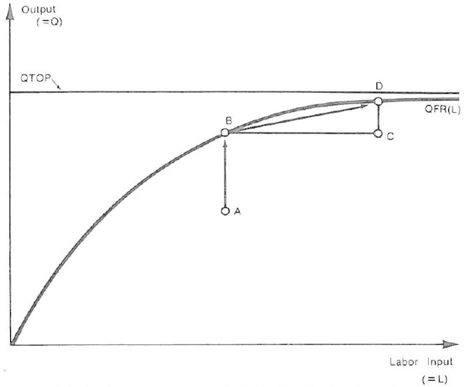
Production system (one firm). The function describing the production system of one firm at one point in time is . How this function is estimated and how it shifts in time in response to investment is described in Eliasson (1976b), Sect. 4 and Albrecht (1978b).
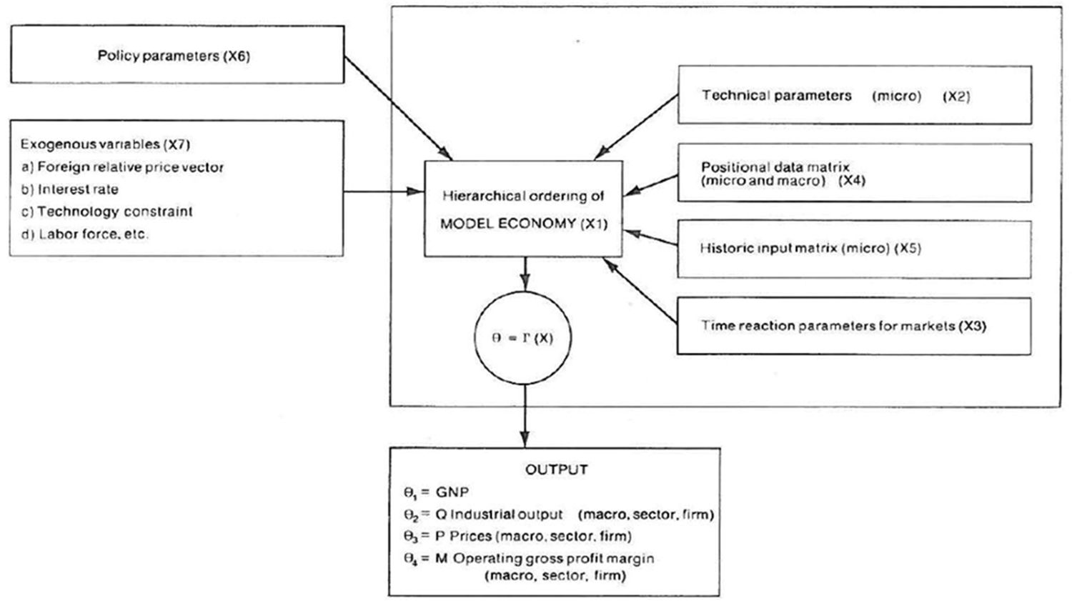
Ordering of variables, policy parameters, and coefficients of entre micro to macro model.
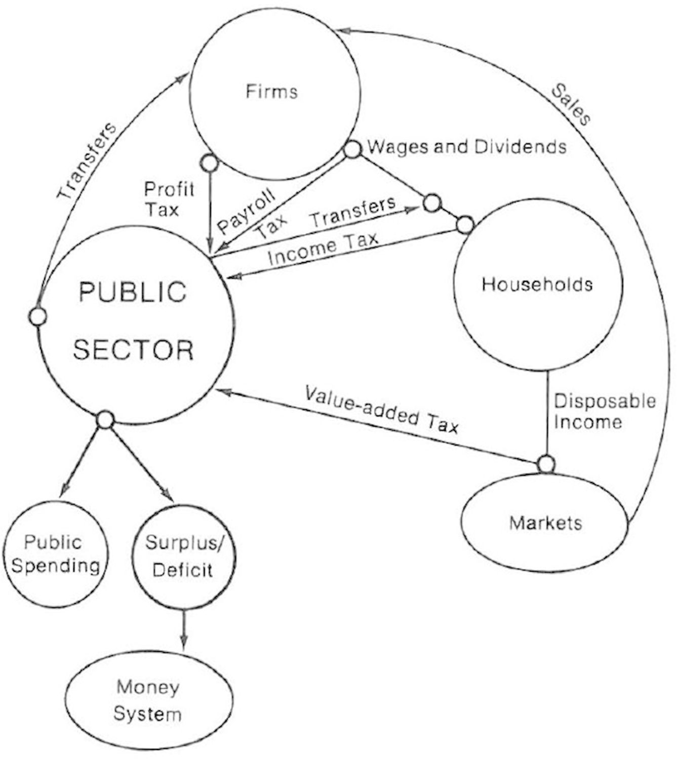
Tax system.

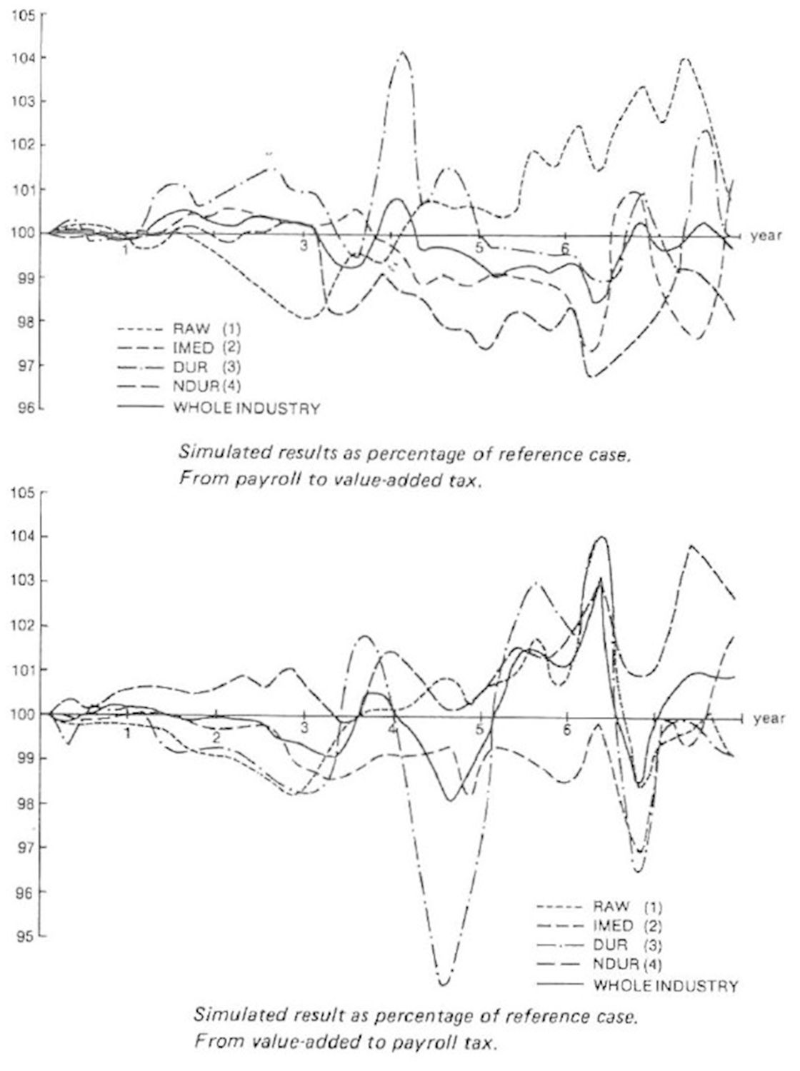
GNP effects of value-added and payroll tax changes. Tax rate changes are up (and down) 2.5% and 5% respectively in the value-added tax case. The payroll tax has been increased and decreased so that the fiscal budget impact the first year is approximately the same as for the corresponding value-added tax change. Simulated results are shown as a percentage of the corresponding values of the reference case.
Sector effects on industrial output of complete change of tax over 5-year period. (See Table 2).

Relationship between rates of return (RR) and growth in output (DQ) of individual firms in the market. The upper graph is a comparison between periods 1969-1975 and 1969-1975, of 5 and 7 year averages respectively. The loweer graph covers the period 1969-1975 before and after the combined transfer payments (to households) and the payroll tax change..

Rates of change in a nominal wage costs to firms (DW) and real rates of return (RR) after inflationary period in investment goods sector. Arrows bind together individual firms and indicate directions of change.
Tables
Effect of Temporary Lowering of Value-added Tax by 3 Percentage Points, 2nd and 3rd Quarters 1974
| After | After2 | 4 | 8 | 12 | quarters |
|---|---|---|---|---|---|
| GNP* | 0 | +0.3 | +0.2 | +0.3 | Percentage points higher |
| Industrial employment | 0 | +0.4 | +0.1 | +0.2 | Percentage points higher |
| Consumer price index (CPI) (incl. value-added tax) | -3 | -0.1 | -0.1 | -0.1 | Percentage points lower |
-
*
In Industrikonjunkturen , Spring 1974:52-53 (Federation of Swedish Industries) , published before the temporary value added tax change, the GNP effrect of a 5-month reduction in the value added tax was estimated to be 0.2 percent on a 12-month basis.
"Budget Neutral" Changes between Payroll and Value-added Tax Systems
| A | B | C | ||||
|---|---|---|---|---|---|---|
| Toward More Payroll Tax* (TWX up 0.05 and TXVA down 0.03 in 1969) | Toward More Valued (Vice-versa) | Value-added Tax Replaces Entire Payroll Tax, over 5-Year Period 1969-1974 | ||||
| Average | 1969-70 | 1969-75 | 1969-70 | 1969-75 | 1969-70 | 1969-75 |
| W cost to firm | 100.8 | 101.6 | 100.1 | 98.8 | 100.0 | 101.8 |
| Take home W | 95.7 | 96.5 | 105.1 | 103.8 | 104.2 | 115.5 |
| PDOM | 99.5 | 100.2 | 103.8 | 104.1 | 101.4 | 107.7 |
| PDOM net of VATAX (to firm) | ||||||
| 102.5 | 103.2 | 100.8 | 101.1 | 100.0 | 101.8 | |
| M | 104.5 | 104.0 | 99.8 | 101.5 | 98.2 | 99.0 |
| CPI | 98.2 | 98.7 | 102.9 | 102.7 | 101.2 | 106.2 |
| CPI net of VATAX | 100.2 | 101.7 | 99.9 | 99.7 | 99.8 | 100.4 |
| PROD | 100.1 | 99.0 | 100.5 | 99.5 | 99.6 | 100.5 |
| Q | 100.3 | 100.3 | 98.8 | 99.6 | 100.2 | 99.9 |
| GNP | 100.9 | 101.0 | 98.8 | 98.7 | 100.0 | 100.1 |
| L | 100.0 | 101.3 | 98.4 | 100.0 | 100.6 | 99.4 |
| RSAVH | 126.7 | 109.5 | 68.3 | 91.3 | 143.3 | 119.0 |
| INVFIX | 110.0 | 106.9 | 100.5 | 94.1 | ||
| EXPORTS | 99.7 | 96.5 | 99.1 | 100.0 | 100.2 | 100.0 |
| Sector Effects (Q) | ||||||
| RAW (1) | 99.8 | 100.0 | 99.1 | 101.0 | 99.9 | 100.6 |
| IMED (2) | 100.0 | 99.2 | 99.5 | 99.8 | 100.1 | 99.7 |
| DUR (3) | 99.9 | 98.1 | 99.0 | 99.8 | 100.4 | 100.6 |
| NDUR (4) | 101.1 | 103.2 | 97.0 | 98.0 | 100.0 | 98.9 |
| Note: For explanation of the scaling see Table 2. | ||||||
-
*
Parameter change determined so that fiscal neutrality obtained first period (quarter) in A and B approximately obtained for 5-year period C. For all remaining periods, differences in the total public tax intake depend on changes in the various tax bases caused by the parameter changes.
Swedish Taxes (thousand Swedish Crownsa).
A B C.
| Skilled Blue-Collar Worker | Well-Paid Salaried Worker | Taxes on Salaried Worker’s Marginal Income above Skilled Blue-Collar Worker | ||||
|---|---|---|---|---|---|---|
| 1969 | 1975 | 1969 | 1975 | 1969 | 1975 | |
| Annual wage (salary), cost to firm | 28.5 | 56 | 63 | 118 | +34.5 | +62 |
| After deduction of payroll tax (WTAX) | 25.5 | 45 | 57 | 100 | ||
| Income tax (ITAX) | 7 | 14 | 24 | 52 | ||
| Transfer income (TRANS) | 4 | 7 | 2 | 3 | ||
| DISPOSABLE INCOME | 22 | 38 | 35 | 51 | +13 | +13 |
| Disposable income as % of wage cost (1) above | 77% | 68% | 56% | 44% | 38% | 21% |
| Savings ratio b (macro), % | 3% | 10% | 3% | 10% | 3% | 10% |
| Value-added tax (VATAX), % on consumption expenditure | 10% | 15% | 10% | 15% | 10% | 15% |
| Returned to firms in the form of demand, in % of total amount paid out | 67% | 52% | 49% | 33% | 35% | 16% |
-
Note: Column C gives the same information as in the preceding columns but tax rates, etc., are calculated on the extra income the salaried worker earned above the skilled blue-collar worker, or 118-56=62 thousand crowns in 1975.
-
a1 Swedish Crown = $0.21 on January 24, 1978.
-
bThe same average savings ration for each year has been applied throughout columns A, B, and C. Savings data for different income groups or estimates on marginal savings rations are not available.
Sensitivity Analysis with Value-added and Payroll Taxes.
| GNP | Industrial Output (Q) | Industrial Employment (L) | CPI | Producer Prices (PDOM) | Wage Costs (W) | Profit Margins (M) | |||||||||
|---|---|---|---|---|---|---|---|---|---|---|---|---|---|---|---|
| 1969- 1970 | 1969- 1975 | 1969- 1970 | 1969- 1975 | 1969- 1970 | 1969- 1975 | Year 7 | 1969- 1970 | 1969- 1975 | 1969- 1970 | 1969- 1975 | 1969- 1970 | 1969- 1975 | 1969- 1970 | 1969- 1975 | |
| VATAX | |||||||||||||||
| +5a | 98.5 | 97.5 | 98.4 | 97.6 | 98.1 | 97.8 | 100.1 | 104.6 | 104.4 | 105.3 | 106.0 | 100.1 | 94.4 | 100.6 | 109.3 |
| -5 | 101.3 | 98.6 | 100.6 | 96.6 | 93.3 | 92.4 | 100.0 | 96.6 | 95.5 | 98.2 | 95.8 | 100.1 | 88.9 | 116.4 | 125.5 |
| WTAX | |||||||||||||||
| +5a | 99.2 | 98.2 | 99.2 | 98.4 | 99.6 | 98.4 | 100.1 | 99.6 | 99.5 | 99.7 | 99.1 | 100.0 | 95.4 | 98.3 | 106.1 |
| -5 | 101.0 | 101.2 | 101.0 | 100.9 | 100.3 | 100.7 | 100.0 | 100.3 | 100.3 | 100.5 | 100.8 | 100.0 | 99.6 | 102.1 | 102.0 |
| W = Labor cost to firm (wages + all social charges incl. supplementary pension charge) | RSAVH = Household savings ration out of disposable income | ||||||||||||||
| PDOM = Domestic wholesale prices, industrial goods, incl. of VATAX | INVFIX = Investment in industry in constant prices | ||||||||||||||
| M = Operating gross profit margin | VATAX = Value-added tax (money terms) | ||||||||||||||
| CPI = Consumer price index, incl. of VATAX | ITAX = Income tax, income earners (money terms) | ||||||||||||||
| PROD = Average labor productivity | WTAX = Payroll tax including all social charges and ATP-charge (money terms) | ||||||||||||||
| Q = Industrial output | TXVA | ||||||||||||||
| GNP = GNP | TXI = The corresponding nominal rates | ||||||||||||||
| L = Labor input in industry; effective man-hours | TXW | ||||||||||||||
| If nothing else is said, all tables and figures are on index form where the endogenous variable reported (Q, PROD, etc.) is indexed with the reference run as the base. On a current basis: If Q(1972) = 3.363 in the reference run and Q(1972) = 3.681 in the experimental run, the index will say index = 3681/3363 x x100 = 109.5 (Diagrams). On an average basis: The indexes have been averaged from the beginning year 1969 to the year you read in the table. | |||||||||||||||
-
W = Labor cost to firm (wages + all social charges incl. supplementary pension charge); PDOM = Domestic wholesale prices, industrial goods, incl. of VATAX; M = Operating gross profit margin; CPI = Consumer price index, incl. of VATAX; PROD = Average labor productivity; Q = Industrial output; GNP = GNP; L = Labor input in industry; effective man-hours; RSAVH = Household savings ration out of disposable income; INVFIX = Investment in industry in constant prices; VATAX = Value-added tax (money terms); ITAX = Income tax, income earners (money terms); WTAX = Payroll tax including all social charges and ATP-charge (money terms); TXVA, TXI, TXW = The corresponding nominal rates;
-
If nothing else is said, all tables and figures are on index form where the endogenous variable reported (Q, PROD, etc.) is indexed with the reference run as the base. On a current basis: If Q(1972) = 3.363 in the reference run and Q(1972) = 3.681 in the experimental run, the index will say index = 3681/3363 x x100 = 109.5 (Diagrams). On an average basis: The indexes have been averaged from the beginning year 1969 to the year you read in the table.