Dynamic Microsimulations of Regional Income Inequalities in Germany
- Federal Statistical Office (Destatis), Germany
- ZDF Digital, Germany
- University of Duisburg-Essen, Germany
Figures

Modules in MikroSim 2.1.4. Source: own illustration.

Mean income by region in the base scenario.. Note: The figure shows the simulated mean income values from 2011 to 2040. The colors indicate regions: East Germany (blue) and West Germany (green). Source: own illustration.

Gender income gaps by region and scenario.. Note: The figure shows the simulated percentage changes in the gender income gap from 2020 to 2040. The colors indicate regions: East Germany (blue) and West Germany (green), while the line types differentiate between the scenarios: base (solid), university endowments of women adapted men (dotted), and full-time rates women adapted to men (dashed). Source: own illustration.

Gender income gaps in East and West by district type and scenario.. Note: The figure shows the simulated percentage changes in the gender income gap from 2020 to 2040 for rural (left side) and urban areas (right side). The colors indicate regions: East Germany (blue) and West Germany (green), while the line types differentiate between the scenarios: base (solid), university endowments of women adapted men (dotted), and full-time rates women adapted to men (dashed). Source: own illustration.
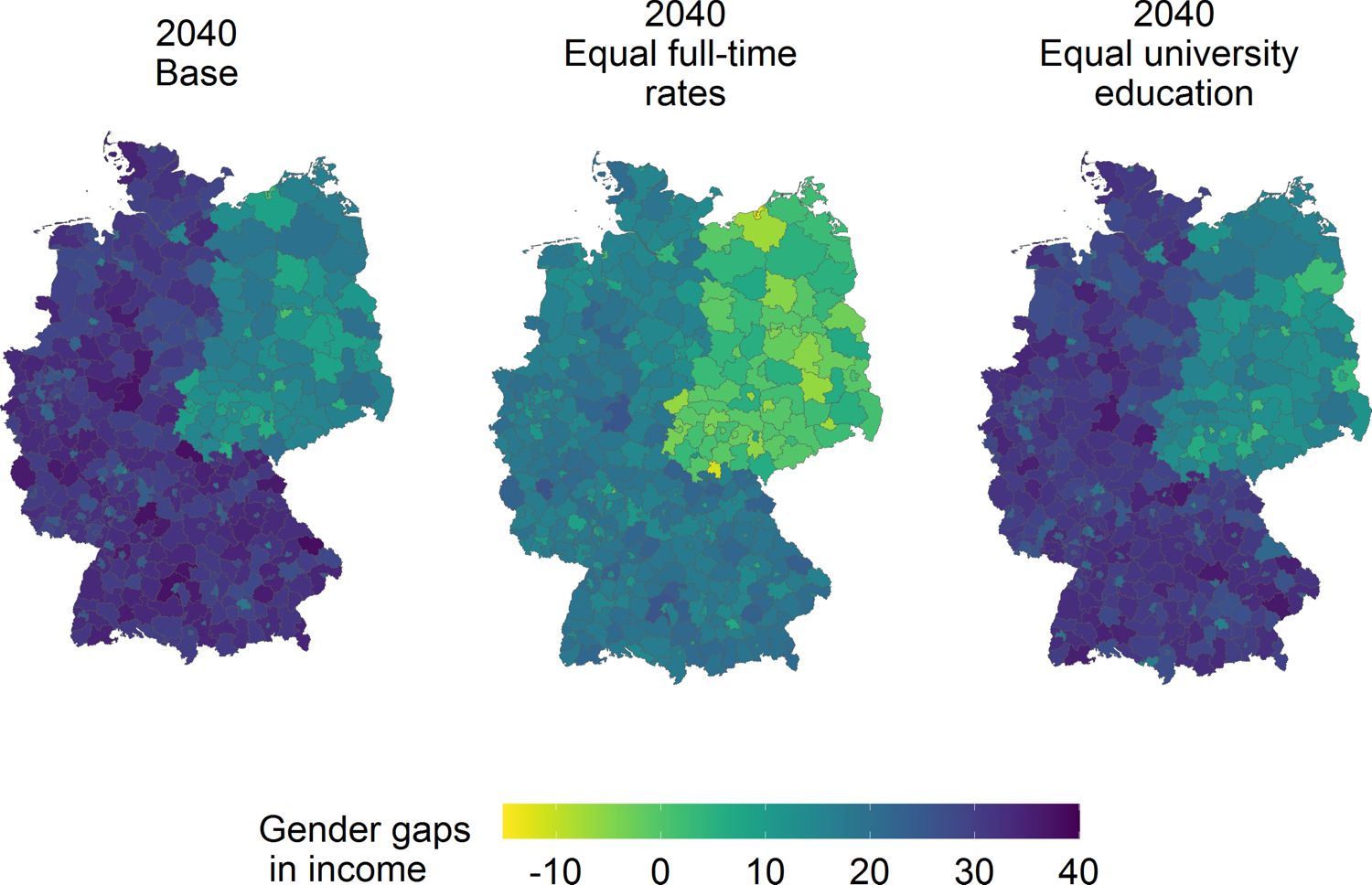
Regional differences in gender income gaps.. Note: The figures illustrate the simulated gender income gaps in 2040 across the 401 German districts under different scenarios: base (left), full-time rates of women adapted to men (middle), and university endowments of women adapted to men (right). Lighter col-ors represent smaller gaps, whereas darker colors correspond to larger wage gaps. Source: own illustration.

Migrant income gaps by region and scenario.. Note: The figure shows the simulated percentage changes in the migrant income gap from 2020 to 2040. The colors indicate regions: East Germany (blue) and West Germany (green), while the line types differentiate between the scenarios: base (solid), university endowments of migrants adapted to the majority population (dotted), and full-time rates of migrants adapted to the majority population (dashed). Source: own illustration.

Migrant income gaps in East and West by district type and scenario.. Note: The figure shows the simulated percentage changes in the migrant income gap from 2020 to 2040 for rural (left side) and urban areas (right side). The colors indicate regions: East Germany (blue) and West Germany (green), while the line types differentiate between the scenarios: base (solid), university endowments of migrants adapted to the majority population (dotted), and full-time rates of migrants adapted to the majority population (dashed). Source: own illustration.
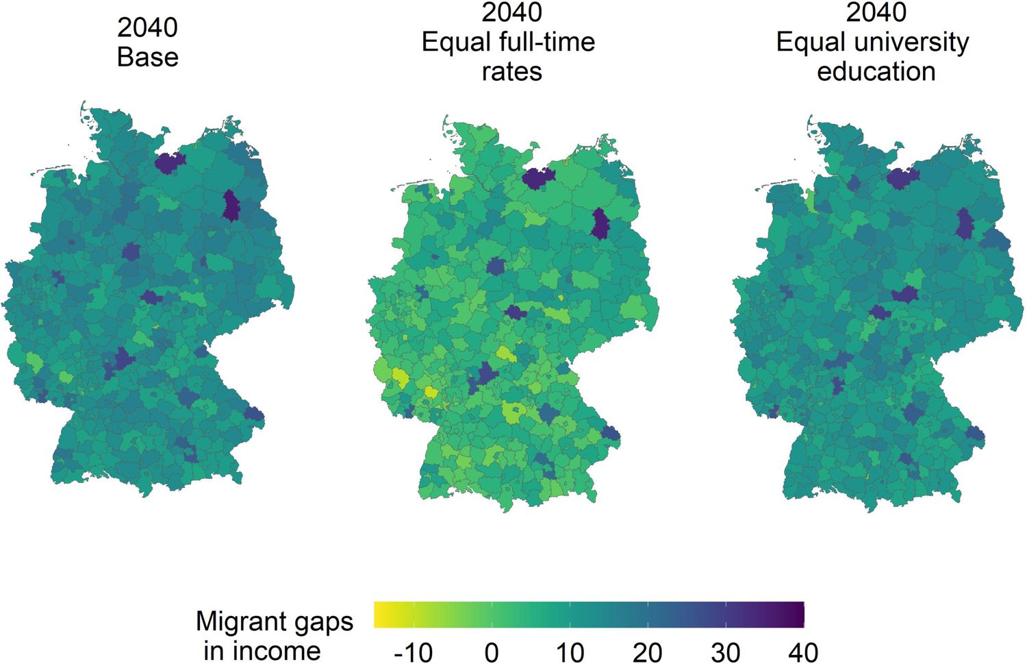
Regional differences in migrant income gaps.. Note: The figures illustrate the simulated migrant income gaps in 2040 across the 401 German districts under different scenarios: base (left), full-time rates of migrants adapted to the majority population (middle), and university endowments of migrants adapted to the majority population (right). Lighter colors represent smaller gaps, whereas darker colors correspond to larger wage gaps. Extreme outliers result from a limited number of observations in some districts. Source: own illustration.
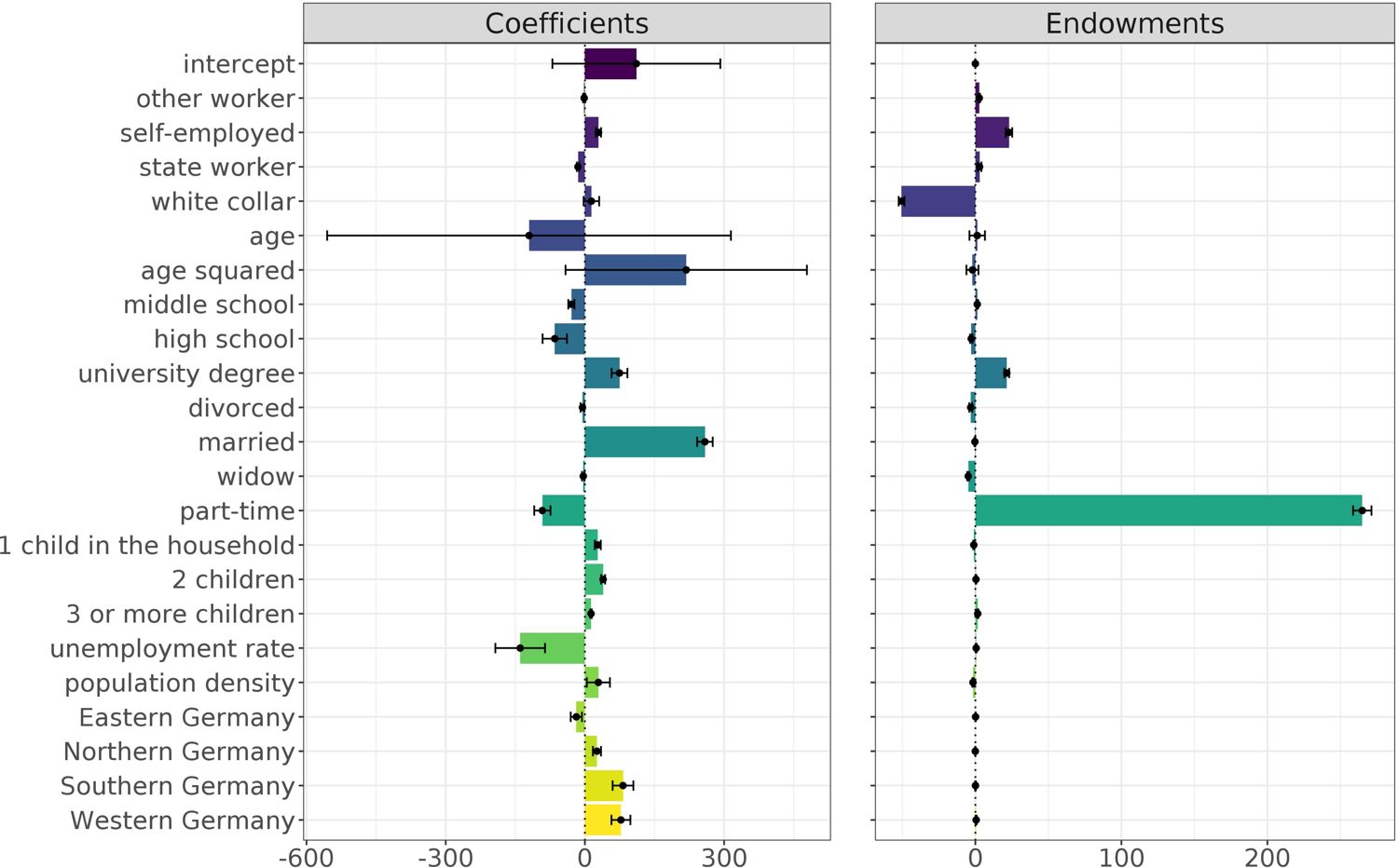
Income gap decomposition by gender15.. Note: The figure shows how far the coefficients (left-hand side) and endowments (right-hand side) widen or narrow the gender income gap. The decomposition results show differences in the magnitude of the coefficients of all independent variables according to gender. While the left-hand side illustrates the effects that narrow the gender income gap, the right-hand side shows the driving forces behind the widening of the gap. The endowments show compo-sitional differences between the sexes. The reducing factors of the income gap are shown on the left-hand side, whereas the drivers of the income gap are illustrated on the right-hand side.For detailed descriptions of the variables and reference categories, see Table A2. Source: own illustration.
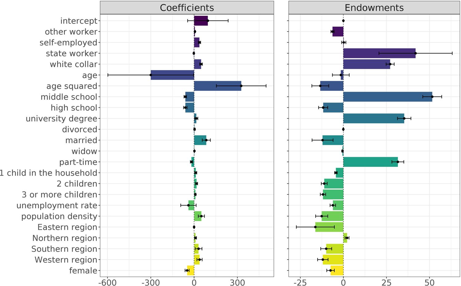
Income gap decomposition by migration status.. Note: The figure shows how far the coefficients (left-hand side) and endowments (right-hand side) widen or narrow the income gap between the migrant and majority population. The decomposition results show differences in the magnitude of the coefficients of all independent variables according to migration. While the left-hand side illustrates the effects that narrow the migrant income gap, the right-hand side shows the driving forces behind the widening of the gap. The endowments show compositional differences between the majority and the migrant population. The reducing factors of the income gap are shown on the left-hand side, whereas the drivers of the migrant income gap are illustrated on the right-hand side. For detailed descriptions of the variables and reference categories, see Table A2. Source: own illustration.

Validation of relative individual income by sex and districts, 2014.. Note: Since the absolute values are on different scales due to the conceptual mismatches and different frames of the underlying datasets, only the comparison of the relative spatial income distributions is meaningful between the three datasets. Darker colors indicate larger individual income medians. Source: own illustration based on Tax Data 2014, INKAR database, and MikroSim.

Working population by region in the base scenario.. Note: The figure shows the simulated working population in millions from 2011 to 2040. The colors indicate regions: East Germany (blue) and West Germany (green). Source: own illustration.

Population by region in the base scenario.. Note: The figure shows the simulated population in millions from 2011 to 2040. The colors indicate regions: East Germany (blue) and West Germany (green). Source: own illustration.

First generation migrants by region in the base scenario.. Note: The figure shows the simulated migrant population in millions from 2011 to 2040. The colors indicate regions: East Germany (blue) and West Germany (green). Source: own illustration.
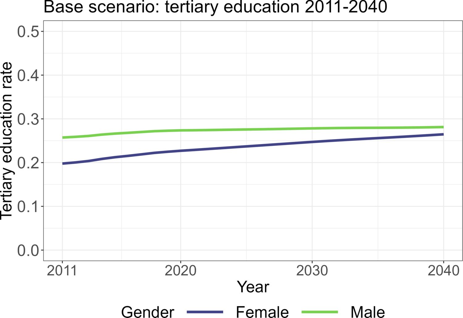
Rate of tertiary education by region in the base scenario.. Note: The figure shows the simulated rate of tertiary education of men (green) and women (blue) in the labor force from 2011 to 2040. Source: own illustration.
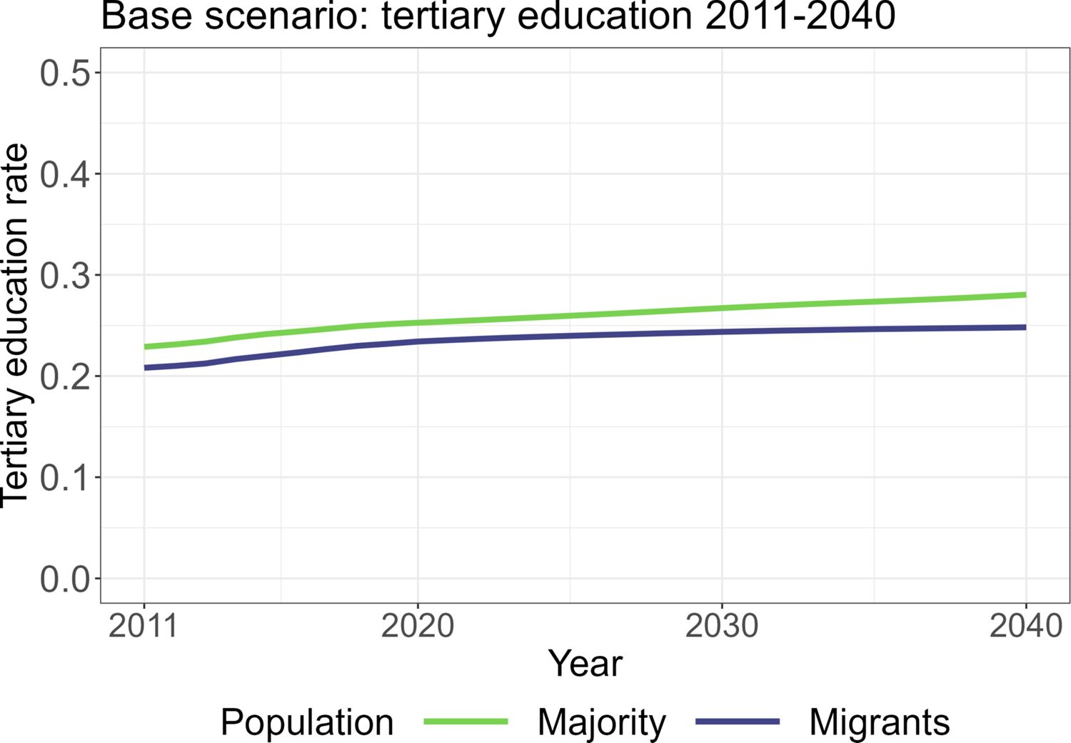
Migrants by region in the base scenario.. Note: The figure shows the simulated rate of tertiary education of the majority population (green) and migrants (blue) in the labor force from 2011 to 2040. Source: own illustration.
Tables
Income Estimation in Selected Microsimulation Models*
| Author & Date | Model | Country | Data | Measure | Estimation | Covariates | Alignment | Regional variables |
|---|---|---|---|---|---|---|---|---|
| Andreassen et al. (2020) | MOSART | Norway | Administrative data registers from Norway | Logarithm of labor income | RE models by different cohorts | Age, gender, partnership status, children, (ongoing) education, seniority, pension (type of pension), stable career path, time outside the labor force, year of observation | Demographic modules are aligned to results from Statistics Norway’s official population projections; for years with actual observations aligned to these | No |
| Bonin et al. (2015) | ZEWDMM | Germany | German Socio-Economic Panel (GSOEP) 2009 data of 25 to 29 aged cohort | Logarithm of gross hourly wage | OLS by gender | Education, working experience, firm tenure | No | No |
| Bönke et al. (2020) | Germany | German Socio-Economic Panel (GSOEP) 1964 to 1985 cohorts until age 60 | Lifetime income (logarithm of labor income) | OLS-LDV by gender | Full- and part-time, employment experience, income from last two years, education, marriage, working hours | No | No | |
| Conti et al. (2023) | T-DYMM | Italy | AD-SILC; administrative and longitudinal survey data | Monthly labor income | RE models by occupational group | Differentiated by groups, complete list: gender, born in EU, education, number and ages of children, working experience, working experience†, permanent contract, part-time, employment status of partner | Demographic modules; income aligned to labor productivity growth and consumer price index | No |
| Dekkers et al. (2009) | MIDAS | Belgium, Italy | Belgium: Panel Households (PSBH); Germany: German Socio-Economic Panel (SOEP); Italy: European Community Household Panel (ECHP) | Logarithm of hourly | Belgium: OLS by germany and Italy: RE by gender | Belgium: Age, age†, education; Germany: Potential experience (= age - years in education), potential experience†, education, marital status, firm size, number of children, chronically ill, tenure, public sector; Italy: Potential experience, potential experience†, education, public sector, permanent contract, duration in work | Corrected growth individual hourly wage rates, additional macroeconomic productivity assumptions | No† |
| Emmerson et al. (2004) | Pensim2 | UK | British Household Panel Survey (BHPS) | Earnings | RE models | Work history (including occupation, industry and sector), year of education | No | No |
| Favreault and Smith (2004); Favreault et al. (2015) | DYNASIM III & MINT8 | US | Survey of Income and Program Participation (SIPP), Panel Study of Income Dynamics (PSID), National Longitudinal Survey of Youth (NLSY) | Logarithm of hourly wages for individuals with positive income for the year | RE models by age, gender and race | Marital status, education level, additional age splines, region of residence, disability status, in school, birth cohort, job tenure, education level*age splines, number and ages of children, health status, disability beneficiary status | Wage growth assumptions are used for future periods | Yes |
| Flood (2008) | SESIM III | Sweden | LINDA administrative panel database; SCB income distribution survey and other | Logarithm of full-time earnings | RE models by occupational sector and gender | Working experience, education, marital status, nationality | Only demographics | No |
| Holm et al. (2007) | SVERIGE | Sweden | Base dataset population of Sweden, ASTRID panel database | Relative earnings (lagged monthly earnings divided by the average earnings) | OLS for full- and part-time workers | Age, gender, education, education the year before, regional unemployment rate | Demographic modules are aligned to aggregate indicators from observed data and projections from Statistics Sweden | Yes |
| Income change (yearly change of earnings) | OLS-LDV for six different groups (got unemployed, emigrated, got employed, immigrated, migrated, ordinary group) | Gender, age, education, civil status, former salary, born in Sweden | ||||||
| Schwabish and Topoleski (2013) | CBOLT | US | Data from the Social Security Administration (SSA), Survey of Income and Program Participation (SIPP), Health and Retirement Survey, Current Population Survey (CPS) | Logarithm of annual earnings | RE (Carroll et al., 1992) | Age, gender, lifetime educational attainment, marital status, number of children u. 6, in school, birth cohort, social security benefit status, permanent and transitory shocks | Modules are aligned to demographic and economic projections from Congressional Budget Office (CBO) | NO |
| Zaidi et al. (2009) | SAGE | UK | British Household Panel Survey (BHPS) | Logarithm of monthly earnings | RE models with first-order disturbance terms by gender and qualifications | Recent employment experience, age, age†, education, occupation, industry, partnership status, employment status of partner, restriction of work by health, public or private sector, children living at home, age of youngest child; full- and part-time status | It is possible to add alignment parameters in future versions of the SAGE model. | No |
-
*
This table is not a complete list of all microsimulation models with income modules worldwide, but an attempt to shed light on the "black boxes" of relevant and ongoing microsimulation models. We have only included microsimulation models that can be cited and provide all information for the table shown
-
†
The updated version of MIDAS-BE 2.0 includes regional information on Flanders, the Walloon area and Brussels-Capital region (Dekkers et al., 2023).
Definition of Covariates
| Individual Characteristics | |
|---|---|
| occupational group | blue-collar (reference), other worker, self-employed, |
| state worker, white collar, | |
| age | age in years |
| education | ISCED levels 1 and 2 (middle school), ISCED level 3 (high school), |
| ISCED level 4 (reference), ISCED levels 5 and 6 (= university degree) | |
| family type | divorced, married, widow, single (reference) |
| part time | 1 if individual works part-time, 0 otherwise (full-time) |
| migrant group | born in Germany (reference), late resettlers, |
| Turkey, South-EU, EU before 2004 (without South-EU) | |
| EU after 2004 (including Poland and Croatia), | |
| Former yug. Countries (without Croatia), Africa, | |
| Near and Middle East, South and South-East Asia, | |
| Rest of the world (incl. Russia, America, Rest of Europe) | |
| female | 1 if individual is female, 0 otherwise |
| Household Characteristics | |
| number of kids | 0 (reference), 1, 2, 3 or more |
| Regional Characteristics | |
| share of unemployed | Unemployed persons per 1000 working-age population (Unemployedtime/Employed(15− < 65 years)time * 1000) |
| population density | Inhabitants per squared kilometer inhabitantstime/areatimecontinuous |
| 5 regions of federal states | North, East, South, West, City-States (reference) |
-
Note: *employees are only employees subject to social insurance at the workplace.
Initial income estimation results for men and women
| Dependent variable: | ||
|---|---|---|
| Log Monthly Income | ||
| Male | Female | |
| Intercept | 6.125*** (0.011) | 5.853*** (0.013) |
| Other Worker | 0.397*** (0.003) | 0.276*** (0.004) |
| Self Employed | 0.094*** (0.002) | 0.096*** (0.004) |
| State-Worker | 0.280*** (0.003) | 0.554*** (0.005) |
| White Collar | 0.098*** (0.001) | 0.185*** (0.002) |
| Age | 0.058*** (0.0005) | 0.065*** (0.001) |
| Age Squared | 0.001*** (0.00001) | 0.001*** (0.00001) |
| ISCED Levels 1 and 2 | 0.326*** (0.003) | 0.331*** (0.003) |
| ISCED Level 3 | 0.116*** (0.002) | 0.154*** (0.002) |
| ISCED Level 5 | 0.142*** (0.003) | 0.088*** (0.003) |
| Late resettlers | 0.095*** (0.004) | 0.073*** (0.004) |
| Turkey | 0.069*** (0.005) | 0.101*** (0.008) |
| South-EU | 0.094*** (0.007) | 0.084*** (0.010) |
| EU before 2004 | 0.054*** (0.009) | 0.028** (0.011) |
| EU after 2004 | 0.147*** (0.005) | 0.112*** (0.006) |
| Former Yugoslavia | 0.113*** (0.008) | 0.081*** (0.010) |
| Africa | 0.220*** (0.012) | 0.105***(0.020) |
| Middle East | 0.123*** (0.008) | 0.089***(0.010) |
| South-East-Asia | 0.169*** (0.010) | 0.157*** (0.011) |
| Rest of the World | 0.127*** (0.007) | 0.126*** (0.007) |
| Married | 0.157*** (0.002) | 0.160*** (0.003) |
| Divorced | 0.013*** (0.003) | 0.055*** (0.003) |
| Widow | 0.119*** (0.009) | 0.223*** (0.003) |
| Part-time | 0.542*** (0.002) | 0.457*** (0.002) |
| 1 Child in Household | 0.036*** (0.002) | 0.037*** (0.002) |
| 2 Children in Household | 0.104*** (0.002) | 0.037*** (0.003) |
| 3 or more Children | 0.159*** (0.004) | 0.032*** (0.005) |
| Unemployment Rate | 0.002*** (0.0001) | 0.002*** (0.0001) |
| Population Density | 0.00003*** (0.00000) | 0.0001*** (0.00000) |
| East | 0.120*** (0.004) | 0.008(0.005) |
| North | 0.066*** (0.004) | 0.019*** (0.005) |
| South | 0.088*** (0.004) | 0.006 (0.005) |
| West | 0.089*** (0.004) | 0.011** (0.004) |
| Number of Individuals | 344,463 | 318,102 |
| var(Ind) | 0.157 | 0.193 |
| var(Residuals) | 0.076 | 0.105 |
| Observations | 635,492 | 573,659 |
| Log Likelihood | 340,397.200 | 389,648.800 |
| Akaike Inf. Crit. | 680,864.300 | 779,367.700 |
| Bayesian Inf. Crit. | 681,262.000 | 779,761.800 |
-
Notes: Standard errors given in parenthesis. ∗p<0.05; ∗∗p<0.01; ∗∗∗p<0.001.
Forecast income estimation results for men and women
| Dependent variable: | ||
|---|---|---|
| Log Monthly Income | ||
| Male | Female | |
| Intercept | 3.134*** (0.013) | 2.929***(0.015) |
| Previous Log Income | 0.571*** (0.001) | 0.570***(0.001) |
| Other Worker | 0.271*** (0.004) | 0.198***(0.004) |
| Self Employed | 0.054*** (0.002) | 0.046***(0.004) |
| State-Worker | 0.121*** (0.003) | 0.256***(0.004) |
| White Collar | 0.055*** (0.002) | 0.109***(0.003) |
| Age | 0.004*** (0.0004) | 0.010***(0.001) |
| Age Squared | 0.00003*** (0.00001) | 0.0001***(0.00001) |
| ISCED Levels 1 and 2 | 0.147*** (0.003) | 0.130***(0.003) |
| ISCED Level 3 | 0.048*** (0.003) | 0.063***(0.003) |
| ISCED Level 5 | 0.097*** (0.003) | 0.074***(0.003) |
| University Graduation | 0.014*** (0.003) | 0.029***(0.004) |
| Late resettlers | 0.039*** (0.003) | 0.031***(0.004) |
| Turkey | 0.005 (0.005) | 0.032***(0.007) |
| South-EU | 0.015** (0.006) | 0.024***(0.009) |
| EU before 2004 | 0.023*** (0.008) | 0.006 (0.010) |
| EU after 2004 | 0.062*** (0.005) | 0.035***(0.005) |
| Former Yugoslavia | 0.045*** (0.007) | 0.032***(0.009) |
| Africa | 0.065*** (0.011) | 0.008 (0.020) |
| Middle East | 0.032*** (0.008) | 0.064***(0.011) |
| South-East-Asia | 0.070*** (0.010) | 0.069***(0.010) |
| Rest of the World | 0.062*** (0.007) | 0.050***(0.007) |
| Married | 0.060*** (0.002) | 0.058***(0.002) |
| Divorced | 0.010*** (0.003) | 0.032***(0.003) |
| Widow | 0.048*** (0.008) | 0.128***(0.005) |
| Part-time | 0.286*** (0.002) | 0.265***(0.002) |
| 1 Child in Household | 0.031*** (0.002) | 0.028***(0.002) |
| 2 Children in Household | 0.062*** (0.002) | 0.054***(0.003) |
| 3 or more Children | 0.097*** (0.004) | 0.068***(0.005) |
| Unemployment Rate | 0.001*** (0.00005) | 0.0005***(0.0001) |
| Population Density | 0.00001*** (0.00000) | 0.00002***(0.00000) |
| East | 0.060*** (0.004) | 0.006 (0.004) |
| North | 0.031*** (0.004) | 0.015***(0.004) |
| South | 0.042*** (0.004) | 0.018***(0.004) |
| West | 0.042*** (0.003) | 0.017***(0.004) |
| Number of Individuals | 194,132 | 174,839 |
| var(Ind) | 0.003 | 0.003 |
| var(Residuals) | 0.119 | 0.154 |
| Observations | 307,605 | 272,851 |
| Log Likelihood | 113,292.900 | 134,186.900 |
| Akaike Inf. Crit. | 226,659.800 | 268,447.800 |
| Bayesian Inf. Crit. | 227,053.400 | 268,836.900 |
-
Note: Standard errors given in parenthesis. ∗p<0.05; ∗∗p<0.01; ∗∗∗p<0.001.
Descriptive Statistics of Individual Net Income
| 20%-Q | 40%-Q | 60%-Q | 80%-Q | Mean | SD | |
|---|---|---|---|---|---|---|
| Female | 700 | 1,000 | 1,400 | 1,900 | 1,400 | 1,400 |
| Male | 1,200 | 1,700 | 2,100 | 3,000 | 2,300 | 2,600 |
| Migrants | 800 | 1,200 | 1,600 | 2,200 | 1,600 | 1,300 |
| Majority population | 900 | 1,400 | 1,800 | 2,500 | 1,900 | 2,200 |
-
Note: Q means quantile. SD means standard deviation. Values are provided in Euro and refer to monthly net income (rounded to hundreds) based on generalized Pareto interpolation.
-
Source: Microcensus 2014.
Descriptive Statistics of the Covariates
| Covariates | 2011 | 2040 |
|---|---|---|
| Blue Collar | 7,268,341 | 9,035,568 |
| Other Worker | 6,851,373 | 2,329,589 |
| Self Employed | 3,491,204 | 3,513,550 |
| State-Worker | 1,795,529 | 2,039,539 |
| White Collar | 20,442,203 | 26,469,607 |
| ISCED Levels 1 and 2 | 32,941,690 | 29,983,438 |
| ISCED Level 3 | 16,727,562 | 18,786,855 |
| ISCED Level 4 (post-secondary) | 14,408,798 | 16,856,388 |
| ISCED Level 5 | 4,723,944 | 5,343,423 |
| Single | 32,186,460 | 35,449,969 |
| Divorced | 5,099,718 | 5,954,598 |
| Married | 30,730,796 | 27,663,157 |
| Widow | 1,949,041 | 2,352,947 |
| Part-time | 9,047,698 | 11,373,085 |
| 1 Child in Household | 5,452,759 | 5,461,470 |
| 2 Children in Household | 3,649,681 | 3,598,167 |
| 3 or more Children | 1,770,310 | 2,780,059 |
| City | 5,703,399 | 6,207,812 |
| East | 13,082,995 | 13,012,529 |
| North | 10,290,519 | 10,628,254 |
| South | 22,997,750 | 24,295,421 |
| West | 28,781,700 | 29,496,169 |
| Germans (working age) | 46,644,839 | 45,461,984 |
| Late resettlers | 2,492,969 | 2,195,640 |
| Turkey | 897,308 | 1,444,008 |
| South-EU | 695,417 | 1,175,148 |
| EU before 2004 | 407,257 | 623,370 |
| EU after 2004 | 650,194 | 1,273,984 |
| Former Yugoslavia | 295,555 | 502,382 |
| Africa | 127,658 | 244,669 |
| Middle East | 173,182 | 331,790 |
| South-East-Asia | 180,834 | 365,227 |
| Rest of the World | 535,904 | 917,020 |
-
Note: The table includes only first-generation working-age migrants.
Data and code availability
The authors use data from the German Microcensus, which is available for scientific research on request from the Research Data Centres: https://www.forschungsdatenzentrum.de/en/household/microcensus.
The simulations are based on the data, model and infrastructure of the MikroSim project: