The financial implications of working longer: An application of a micro-economic model of retirement in Belgium
- Federal Planning Bureau, Belgium
- Centre for Sociological Research (CESO), Katholieke Universiteit Leuven, Belgium
- Article
- Figures and data
-
Jump to
- Abstract
- 1. Introduction
- 2. The option value approach
- 3. A comparison between mep and earlier applications of the option value approach
- 4. The two Belgian state retirement schemes
- 5. The Micro-Economic Pension Model (MEP)
- 6. Results
- 7. Conclusions
- The estimation of wage matrices
- References
- Article and author information
Abstract
In this paper, the costs and benefits associated with postponing retirement are simulated in a standard simulation model for Belgium, using the approach of Stock and Wise (1990). Unlike earlier microsimulation-based applications of this approach, such as Gruber and Wise (1999, 2004), this model does not take a representative sample as the point of departure, but simulates the costs and benefits of postponing retirement for four fictitious employees, representing male and female white- and blue-collar workers. While confirming conclusions drawn by other authors, this model allows for the separation of specific retirement schemes, and of the effect of different fiscal regimes for those retired and working. It is shown that differences between retirement schemes show up in differences in replacement rates and by whether or not the retirement benefit is a function of career length. Furthermore, advantageous fiscal regulations for the retired have a strong impact on the implicit costs of postponing retirement.
1. Introduction
As a result of structurally low fertility and ever-increasing life expectancy, the Belgian population is ageing rapidly. The 2004 report of the ‘Studiecommissie voor de Vergrijzing’ (Commission for the Study of Ageing) (High Council of Finances, 2004: 20), estimates the budgetary cost of ageing to be 3.4% of GDP. It also concludes that an effective way to moderate costs would be to persuade individuals to postpone their retirement, as an increase by one year of the average age at which people retire would decrease the budgetary cost of ageing by 0.9% of GDP. In this, Belgium especially faces a challenge. Figure 1 shows the activity rate and effective retirement age of older employees in European countries.
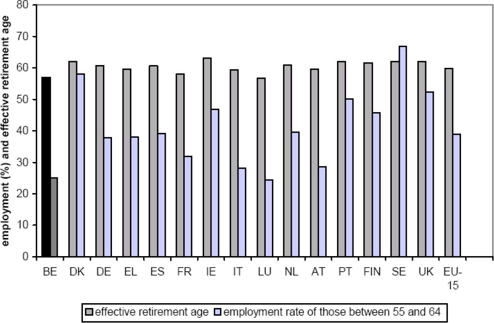
Activity rate of 55–65 year olds, and effective retirement age in Europe (European Community, 2003: 42–48).
For the European Union as a whole, 38.8 % of those older than 55 still have a job. This percentage is 25.1 in Belgium, a figure lower only in Luxembourg. The effective age of retirement is 59.9 in Europe as a whole, and 57 in Belgium. The European countries decided at the European Summit in Barcelona in 2002 that this effective retirement age should be increased by five years before 2010 (EC, 2003). This clearly is even more important for Belgium than for other countries.
The purpose of this paper is to provide an insight into what extent the current public retirement schemes for private-sector wage earners might encourage older workers to voluntarily leave the labour market and enter retirement. What is the penalty for continuing to work? And does this differ between workers of different categories, and between the two main public retirement schemes available in Belgium? These questions are to be answered exploiting the so-called option-value approach. The model to be presented in this paper is based on the notion of actuarial non-neutrality (OECD, 2003: 4) of a retirement scheme, setting the gains from postponing retirement (extra salary) against the losses (foregone expected pension, for all future years until decease) associated with a specific retirement scheme. The which its simulation results will be discussed at length. Finally, conclusions will be drawn.
2. The option value approach
The well-known replacement ratio compares the last-earned salary with the pension benefit one receives immediately after retirement. This may not be the best variable to reflect a retirement decision, for two reasons. First, it is based on pension benefit in the first year after retirement, and ignores the future development of pension benefit conditional upon the year of retirement. Second, it suggests that working and retirement are two exchangeable strategies, i.e. that a retired individual can re-enter the labour market in any future year. Although this may be theoretically possible, in practise such behaviour is rare. Hence Duval (2003: 34) describes retirement as an “absorbing rather than as a dynamic state”.
The option value approach, developed by Stock and Wise (1990) supposes that a representative agent considers the gains and losses in utility pertaining to every year that he or she could retire. He or she weighs the utility of consumption (i.e. the higher income when working) against leisure (retirement). In this, he or she does not compare just the current alternative incomes, but the expected value of all current and future incomes. Define t as the first year that our individual has the institutional possibility to retire, and define r ≥t as the year that he or she retires. The flow of expected future utilities can then be written as:
| t | the year of potential retirement |
| r | the year of actual retirement |
| s | future year, starting from either t or r |
| ys | labour income or salary in year s |
| bs(r) | pension income in year s, given retirement in r |
| Uy | the utility of consumption |
| Ub | the utility of leisure |
| β | discount factor = 1/(1+discount rate) |
| as | the probability of survival from t to s |
Given that r* = arg max(Vt(r)), it holds that Vt(r*) − Vt(r) > 0 for each year that r* ≠ r. Considering all the future years that one can choose to retire (i.e. from t to the year one reaches the mandatory retirement age), the option value in t is Gt(r*) = Vt(r*) − Vt(t), and one will postpone retirement from year t for as long as Gt(r*) > 0. In r*, there is no additional expected utility from working, and one will therefore retire. Following Gruber and Wise (2004: 26), the option value can be rewritten as
or
As defined the option value and peak value both assume that the older worker considers all years from t to the legal retirement age in one decision. One might, however, also want to consider year-to-year decisions, in which one decides (not) to retire just for the year to come. This decision is reflected by some additional variables, closely related to the above option and peak value, which are to be presented now. First of all, Social Security Wealth (SSW) can be expressed as the flow of discounted expected utility from retirement in the year r, as seen from t:
The change of SSW as a result of postponing retirement by just one year, is
This is referred to as the wealth accrual. When retirement is postponed by one year, one renounces one year of pension benefits. However, depending on the scheme, the pension benefit may be a function of the career length, and postponing retirement then implies a higher benefit in the remaining years of retirement. If the two effects cancel each other out for an additional year of work, the system is said to be “actuarially neutral at the margin” (OECD, 2003: 34). In practice, however, the first effect usually outweighs the second one (not least because of discounting), so usually ∆SSWrt < 0, in which case continuing to work comes with a loss in pension wealth (i.e. total post-retirement pension income).
The option value and peak value reflect a retirement decision to be taken about all the future years from t to the year one reaches the mandatory retirement age. The wealth accrual describes a year-to-year retirement decision, but considers only pension income and neglects labour income. One may therefore want to add variables that compare discounted salaries and pension incomes in a year-to-year-retirement decision.
Write PR as the balance of discounted salaries and changes in pension wealth that result from postponing retirement by one year:
This variable is the balance of expected gains (one additional year of salary) and losses (a decrease of the stream of future pension benefits) if one postpones retirement in r. Income earned usually outweighs the negative wealth accrual, and therefore PRt(r) is usually positive. Gains associated with continuing to work will often outweigh the losses, but we shall see that these increases in wealth as a result of continuing to work are (sometimes considerably) lower than the salary suggests. This may help to account for the fact that that a proportion of wage-earners chooses not to work but to retire instead. Note again the strong relation between the single- and multiple-year retirement decisions; PR and SSW are the single-year ‘versions’ of the option value and peak value.
A second additional variable is used by the OECD (2003: 34), Duval (2003: 18), Börsch-Supan (2000:31) as well as Nelissen (2001: 5) and is referred to as the ‘implicit tax on working through r’. For every year that retirement is postponed, the ratio of expected losses (renounced pension wealth) and gains (salary), shows that the former presses as an implicit tax on the latter.
Following the same line of reasoning explaining that PR usually is positive, one can expect itax to be usually positive as well. If not, it is to be interpreted as an implicit subsidy on work.
3. A comparison between mep and earlier applications of the option value approach
The option value approach has been applied in several studies to date. The best known is that of Gruber and Wise (2004), in which the probability that one retires at a certain age is regressed on wealth accrual, peak value and option value. A similar study has been undertaken by Dellis et al. (2004: 41) for Belgium. The broad conclusion is that, even though the estimators of all variables are significant, wealth accrual has the highest explanatory value for both men and women. Subsequently these models have been used to simulate the effect of policy measures on the retirement probability.
The OECD (OECD, 2003; Duval, 2003) also uses this approach to simulate and compare the actuarial nonneutrality of retirement schemes between countries. Their conclusion is that the implicit tax on continuing to work is low for workers of 55-years old, but increases considerably with age. Countries differ significantly, and these differences coincide with differences in replacement ratios.
Similarly, Börsch-Supan (2000) explains labour market status (retired or working) using a regression model, including option value with gender, health, education, age and pension-type. This model is estimated on German data and the results were used to simulate the impact of actuarial changes in retirement benefits on retirement age. In later work, Berkel and Börsch-Supan (2003) concentrate on institutional characteristics of the German retirement system, and simulate the effect of implementing a system of Notional Defined Contributions (NDC) on the effective retirement age.
The above papers all present models which can be classified as static microsimulations (Van Mechelen & Verbist, 2005), for the calculation of the option values are made for a representative sample, and then regressed on the probability that an individual retires. This means that information on specific alternative retirement schemes are combined for existing individuals, and that the information on different individuals is combined in the estimation results. In contrast, the Micro-Economic Pension model (MEP) to be presented in this paper may be classified as a standard model. As in a conventional microsimulation model, the point of departure is the individual; but a standard simulation model concentrates on the calculation of the various indicator variables for four fictional individuals representing male and female blue- and white-collar private-sector wage earners. It also includes two separate ‘first-pillar’ (state) retirement schemes – the early retirement scheme and a conventional early leavers’ scheme. Instead of aggregating outcomes across these schemes and types of individual, MEP keeps them separate, so that comparisons can be made as to the actuarial non-neutrality of the two retirement schemes with respect to male or female white- or blue-collar workers, and the degree to which these schemes may stimulate a step into retirement. Furthermore, an explicit goal of MEP is to bring to the fore the effect of different tax regimes on the implicit costs of continuing to work. For this reason we follow the two OECD studies (OECD, 2003; Duval, 2003) in expressing the variables presented above in monetary units rather than in terms of utility. The advantage of this approach is that it prevents the simulation results being determined to some degree simply by assumptions concerning the difference in utility between a salary or a pension benefit of one euro. Moreover, it is in line with the widely used replacement ratio, which is also a ratio of currency-units. Finally, MEP does not include a behavioural equation relating the option value variables with effective retirement probabilities. So, a higher (lower) implicit cost of retiring is assumed to encourage (discourage) retirement, but it is unknown by how much exactly.
4. The two Belgian state retirement schemes
The Belgian retirement system consists of three pillars. The first pillar is provided by public social security programs, which are the most important source of income for current pensioners. The second pillar is that of company pension schemes. Although coverage of these schemes is increasing rapidly, their importance in terms of the income they provide to current pensioners is still limited. The third pillar consists of individual life-insurances and retirement savings. We concentrate upon the first-pillar social security retirement schemes. Ignoring disability schemes, older private-sector wage earners have two ways of retiring before the mandatory age of retirement. The first is via the system of early retirement (‘vervroegd rustpensioen’), and the second is via the conventional early leavers’ scheme (‘brugpensioen’) hereafter abbreviated to CELS. Both will be explained in broad lines in this section.
The retirement system provides former private sector employees a pension benefit which essentially is a function of their past career. The mandatory age of retirement is 65 for males. For females it is gradually increasing from 61 years of age (from July 1997) via 63 years (from 2003 on) up to 65 (from 2009 on). Males become eligible for early retirement from the age of 60 on, if they have a minimum career service 35 years. For females, this minimum career length increased from 20 years in 1997 to 34 years in 2004, and is set to increase further, to 35 years, in 2009. Males and females can in principle therefore retire, and start to drawn public social security pensions, 5 and 3 years before the mandatory retirement age. The remainder of this paper seeks to identify the implicit costs associated with working through to the mandatory retirement age rather than exercise the optional right to retire early.
State pension benefit is calculated as
The wage-base is essentially the sum of past salaries, indexed on the development of prices and with additional discretionary adjustments for the development of wages between the year of earning and the year of retirement. This modified sum of corrected salaries is then multiplied by the length of the career and divided by the length of the career needed for a full pension. The latter equals the age at which one becomes eligible to a full pension benefit minus 20. So, for males, it is 65 – 20 = 45 years. For females, it is gradually increasing to 45 years. As a result, if one does not have a full career, continuing to work causes the pension benefit to move towards the ‘full-career pension benefit’. This wage-base is then multiplied by either 60% or 75%. If the individual is single, 60% is used. If they have a partner, they can choose the ‘family pension benefit’ of 75%, but then their partner loses his or her own pension entitlement. In consequence, this choice is only beneficial if one’s partner has no significant revenues of his/her own.
Redistributive solidarity is embedded in the pension system in several ways. First of all, the wage one earns in a certain year during one’s career is taken into account only up to a certain limit. All incomes higher than this limit do not add to the wage-base, and hence not to the future pension benefit. Those earning a higher income therefore face a lower replacement rate. Second, for those with a career of at least 15 years, the wage-base is calculated substituting a minimum annual allowance for periods of low earnings. Third, there is a minimum pension benefit guaranteed to all, modified for those without a full career history.
An alternative to this system of early retirement is the conventional early leavers’ scheme, which is essentially an unemployment scheme. It allows older workers to exit the labour market and become unemployed on favourable terms until the mandatory retirement age. People generally become eligible for a CELS benefit from the age of 58 onwards. (In practice, many older workers retire to the CELS before the age of 60. But these regulations are of an ad hoc nature and therefore not considered further in this paper.) The benefit consists of two parts. First, there is a general unemployment benefit which is equal to 60 % of the last wage up to a ceiling. Second, there is an additional benefit which equals 50% of the difference between the unemployment benefit and the last wage minus taxes and social-security benefits. The CELS benefit decreases relative to increasing income, because (i) regular unemployment benefit is limited, and (ii) the progressive tax-system causes net income to lag behind gross income as the latter increases.
Unlike early retirement benefit, the CELS benefit does not depend on the number of working years. Furthermore, when one enters the CELS, formally one does not retire but becomes unemployed. The career length, on which the future statue pension will be based upon reaching the mandatory retirement age, therefore continues to increase. Note that one may choose to work after retirement, but the additional income one may earn is very limited. Furthermore, returning to work from a situation of retirement is possible in theory, but rarely seen in practice. Finally, switching from the CELS to the early retirement scheme may be possible, but is not rational and therefore never done. Switching in the opposite direction is not possible.
5. The Micro-Economic Pension Model (MEP)
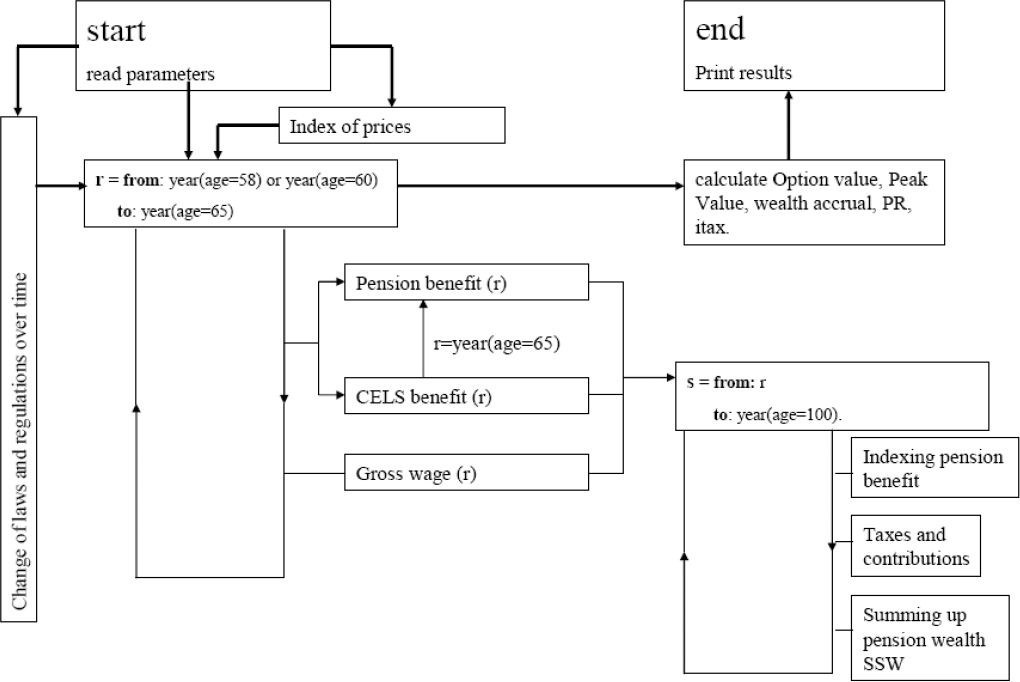
The Micro-Economic Pensions model (MEP) evaluates Equations 2 to 6 for fictitious individuals representing male and female white- and blue-collar workers. The model is written in the SAS macro language and consists of a body of several modules, accompanied by two modules that read time-dependent parameters, such as gross wages, pensions, minimum and/or maximum benefit levels and wage-ceilings, tax and social contribution rates, survival probabilities, inflation rates, and so forth. Figure 2 shows the technical structure of the model.

The structure of the micro-economic pension model.
The discussion of the model starts in the top-left quadrant of Figure 2. The user needs to provide the model with information on the gender and labour market status of the fictitious individual, and whether or not he or she applies for a family pension benefit or a single-person pension benefit. Furthermore, one needs to provide a discount rate, and to decide whether results should be expressed in gross or net amounts.
Using this information, MEP will for every year r ≥ t that the individual is eligible to the pension benefit in question, calculate the flow of future expected pension benefits from all future years s until expected death, using the information available at r. All benefits are then discounted back to t using a discount rate and a survival probability. In the case of the CELS, the social security wealth SSW will sum CELS benefits up to the mandatory retirement age, and pension benefits afterwards.
For the calculation of pension or CELS benefit, as well as the various indicators of actuarial non-neutrality, one needs past and current gross-incomes. The model includes a matrix containing wages per day for every combination of gender and labour market status, for all ages between 20 and 64 and for all the years between 1955 and 2004. The creation of this matrix is discussed in the appendix.
For a thorough understanding of the model, two fundamental assumptions need to be discussed briefly. The first assumption pertains to the set of laws, rules and regulations on pensions, taxes and contributions that an individual faces in a certain year. In any year r, potential retirement benefits for all future years s are derived using information on laws, rules and regulations available at r. Suppose that an individual may choose to retire in 2003. His potential pension benefit in the future year 2010 will be derived using information available in 2003. If he or she postpones retirement and reconsiders in 2004, then the potential pension in the same year 2010 will be calculated using the information available in 2004. The second assumption pertains to the individuals who form the basis of the MEP model. To keep things simple, especially with respect to fiscal laws and regulations, it is assumed that an individual is either single or the sole income earner in the household. In other words, the income of the individual is the only income of their household. A consequence of this is that a married individual will by definition choose the family pension benefit of 75% of the wage-base.
Inputs to the model are based on information drawn from Put (various years) and Ministry of Finance (various years) and follow regulations on taxes, social contributions, pension benefits and CELS benefits for the years 1997–2004. It is assumed that the four typical employees are born in 1940 and enter the labour market at the age of 20. Survival probabilities are derived from the 2000 mortality rates (National Institute of Statistics and Federal Planning Bureau, 2003). Finally, and in accordance with Dellis et al. (2004: 5) and Berkel and Börsch-Supan (2003: 3), the discount rate is set at 3%.
6. Results
6.1 Retirement
Tables 1 to 4 below present the results for a single male or female white- or blue-collar worker.
Pension benefit for a single male white-collar worker.
| age | year | career length | gross wage | gross benefit | gross replacement rate | net replacement rate | net option value (€) | net peak value (€) | net ∆SSW | net PR | net itax |
|---|---|---|---|---|---|---|---|---|---|---|---|
| 60 | 2000 | 40 | 47,811 | 15,763 | 0.330 | 0.519 | 59,255 | −28,838 | . | . | . |
| 61 | 2001 | 41 | 49,534 | 16,600 | 0.335 | 0.522 | 42918 | −23,449 | −5,390 | 17,216 | 0.238 |
| 62 | 2002 | 42 | 50,758 | 17,512 | 0.345 | 0.529 | 27,929 | −16,110 | −7,339 | 14,984 | 0.329 |
| 63 | 2003 | 43 | 51,565 | 18,193 | 0.353 | 0.537 | 13,094 | −8,680 | −7,429 | 14,454 | 0.340 |
| 64 | 2004 | 44 | 52,512 | 18,856 | 0.359 | 0.543 | 0 | 0 | −8,680 | 12,591 | 0.408 |
Pension benefit for a single female white-collar worker.
| age | year | career length | gross wage | gross benefit | gross replacement rate | net replacement rate | net option value (€) | net peak value (€) | net ∆SSW | net PR | net itax |
|---|---|---|---|---|---|---|---|---|---|---|---|
| 60 | 2000 | 40 | 26,260 | 11,402 | 0.434 | 0.683 | 31,744 | −23,272 | . | . | . |
| 61 | 2001 | 41 | 27,171 | 12,057 | 0.444 | 0.690 | 21,256 | −20,234 | −3,039 | 11000 | 0.216 |
| 62 | 2002 | 42 | 27,733 | 12,801 | 0.462 | 0.704 | 12,324 | −15,236 | −4,998 | 8,844 | 0.361 |
| 63 | 2003 | 43 | 28,193 | 13,029 | 0.462 | 0.702 | 6,461 | −7,280 | −7,956 | 5,712 | 0.582 |
| 64 | 2004 | 44 | 28,664 | 13,409 | 0.468 | 0.708 | 0 | 0 | −7,280 | 6,098 | 0.544 |
Pension benefit for a single male blue-collar worker.
| age | year | career length | gross wage | gross benefit | gross replacement rate | net replacement rate | net option value (€) | net peak value (€) | net ∆SSW | net PR | net itax |
|---|---|---|---|---|---|---|---|---|---|---|---|
| 60 | 2000 | 40 | 22,541 | 10,833 | 0.481 | 0.734 | 23,179 | −24,162 | . | . | . |
| 61 | 2001 | 41 | 23,205 | 11,365 | 0.490 | 0.748 | 15,894 | −19,531 | −4,631 | 7,678 | 0.376 |
| 62 | 2002 | 42 | 23,489 | 11,963 | 0.509 | 0.768 | 10,245 | −13,093 | −6,438 | 5,536 | 0.538 |
| 63 | 2003 | 43 | 23,832 | 12,395 | 0.520 | 0.771 | 4,972 | −6,662 | −6,431 | 5,296 | 0.548 |
| 64 | 2004 | 44 | 24,128 | 12,840 | 0.532 | 0.790 | 0 | 0 | 662 | 4,690 | 0.587 |
Pension benefit for a single female blue-collar worker.
| age | year | career length | gross wage | gross benefit | gross replacement rate | net replacement rate | net option value (€) | net peak value (€) | net ∆SSW | net PR | net itax |
|---|---|---|---|---|---|---|---|---|---|---|---|
| 60 | 2000 | 40 | 13,662 | 8,187 | 0.599 | 0.785 | 19,236 | −13,706 | . | . | . |
| 61 | 2001 | 41 | 14,056 | 8,856 | 0.630 | 0.828 | 9,189 | −15,512 | 1,806 | 10,302 | −0.213 |
| 62 | 2002 | 42 | 14,285 | 9,438 | 0.661 | 0.861 | 4,466 | −11,856 | −3,656 | 4,642 | 0.441 |
| 63 | 2003 | 43 | 14,475 | 9,438 | 0.652 | 0.831 | 6,707 | −1,405 | −10,451 | −2,299 | 1.282 |
| 64 | 2004 | 44 | 14,682 | 9,992 | 0.681 | 0.873 | 0 | 0 | −1,405 | 6,563 | 0.176 |
Table 1 presents the results for a single male white-collar worker. The year 2000 (at the age of 60) is the first year in which he can choose to retire. If he continues to work through this year, his gross income will be 47,811 euro. If he decides to apply for a pension benefit, this gross benefit will amount to 15,763 euro. The second row contains this information if he decides to work through 2000 and reconsider retirement in 2001 (i.e. at the age of 61). The ratio of alternative incomes, hereafter loosely called the replacement ratio, lies around 34%. That this is below 0.60, the fraction by which the pension base is multiplied to calculate the pension benefit, is caused by the fact that the pension benefit is based on the average (adjusted) wage over the length of the career, and given a maximum. Especially for male white-collar workers, the salary increases with age. The wage earned in the last year of the career is therefore higher than the average wage, and the ‘replacement ratio’ ends up well below 60%. The replacement ratio increasing with age is caused by the increasing career length, causing the pension benefit (the numerator) to increase, combined with the lower growth of the gross salary (the denominator). Finally, the net replacement ratio is 53% on average, and is higher than the gross replacement ratio. This is because of the progressiveness of the tax rate, and of a tax-exemption for retirees. This will be discussed further in Section 6.3.1.
Equation 1 shows Vr to be the expected discounted value of future benefits and salaries if the individual retires in r. When postponing retirement by one year, one roughly loses one year of pension benefits. The future pension benefits for the remaining years of retirement may however increase as a result of the longer career. One moreover gains a years’ salary. The gains outweigh the losses, so total wealth is maximized if one continues to work as long as possible, i.e. max(Vr) = V2004. The option value is therefore positive and becomes zero at r = 2004.
The peak value in the first row of Table 1 shows the difference in the flow of expected discounted benefits if one retires at the age of 60 compared to when one retires at that age where the option value is zero (i.e. at 64). The sooner one retires, the greater the flow of expected future benefits, meaning that the increase of future pension benefit as a result of continuing to work does not fully compensate for the lost pension year. The peak value will therefore be negative and zero at the age of 64. When only pension benefits are considered, one should of course retire as soon as possible.
The three indicators to be discussed next consider a year-to-year retirement decision. The variable ∆SSW reflects the loss in expected flow of pension benefits if retirement is postponed by one year. One can expect ∆SSW<0 for the same reason as for the peak value. Table 1 shows that this net loss of postponement is more than 5000 euro in the first year, and increasing. So there is reason to retire as soon as the possibility arises. However, one does not only lose when postponing retirement; one gains salary as well. The variable PRr shows the balance between the two alternatives. It again shows that the profit of postponing retirement decreases with age, especially between the first and second year. The last indicator itaxr shows the loss (the sum of lost future expected discounted pension benefits) as a fraction of the gain (salary). The advantage of this indicator is that it does not have a scale, and this will turn out to be convenient when the results are to be compared with those of other representative individuals. As PR is positive, itax will usually be positive as well, meaning that there is an implicit tax on working longer. In the first year, this implicit tax is almost 24%, but increases immediately to almost 33% in the second year. After that, the increase continues, albeit at a lower speed. The conclusion again is that retirement is encouraged, and that implicit taxes increase with age.
Comparing Table 1 with Tables 2 (female white-collar workers) and 3 (male blue-collar workers) reveals that both the gross and net replacement rate are inversely related to income. There are two explanations for this. First, the increase of wage with age is higher for male white-collar workers than for female white-collar workers and blue-collar workers (see appendix). The average income will therefore be further below the last wage for the first category compared to the last two, and hence the difference in the replacement ratio. Second, as male white-collar workers have the highest income, the effect of the upper wage limit in the calculation of the wage-base (and therefore the pension) is more important, causing the replacement rate to be lower.
Compared to the figures in Table 1, incomes, profits and losses of postponing retirement, and therefore the indicators, are all lower in Tables 2 and 3. In contrast the implicit tax rate itax has no scale. Two effects explain the change of the implicit tax rate between categories of employees. The first, relating to the change of itax between male blue- and white-collar workers, is that the implicit tax rate increases with the replacement ratio (cf. Börsch-Supan, 2000: 131; Duval, 2003: 33). The second, relating to the difference between male and female white-collar workers, is that the loss associated with postponing retirement is especially high for females. This is because the length of career required for a full pension benefit is shorter for women than for men, although increasing over time. As the year of entering the labour market is assumed to be the same for all typical individuals whose simulations are discussed, female employees reach a full pension before males. If full career is reached, postponing retirement no longer results in an increase in the pension benefit for the remaining retirement years. The profit associated with postponing retirement therefore decreases, and the implicit tax increases.
The results for female blue-collar workers are discussed separately. With the employee-types discussed so far, the loss of one year of pension benefits as a result of postponing retirement outweighed the gain in the higher pension benefit in the remaining years. As a result ∆SSW was negative, and itax was therefore positive as well. In the case of female blue-collar workers, this is no longer the case, as their pension benefit is not a function of the wage, but of the minimum pension benefit set by law. The effect of postponing retirement is therefore determined by the development of this minimum pension over time. If a female blue-collar worker postpones retirement from 2000 to 2001, the minimum pension benefit given a full career will have gone up considerably. Moreover, the woman does not have a full career and the effective minimum benefit level is decreased pro rata temporis. Postponing retirement therefore results in the effective minimum pension benefit increasing even further. This causes the profit of postponement to outweigh the loss, and thus results in an implicit subsidy (a negative implicit tax) on labour of 21%. In later years, the situation is back to normal in that itax>0. This is because of the lower increase of the minimum pension benefit over time, combined with the fact that the woman has reached full career. The conclusion therefore is that it is profitable for blue-collar females to continue to work between 2000 and 2001, but highly costly afterwards.
6.2 CELS benefit
Tables 5 to 8 contain the simulation results of the CELS benefit for the four types of employee discussed in this paper.
CELS benefit for a single male white-collar worker.
| age | year | career length | gross wage | gross CELS benefit | gross future pension benefit | gross replacement rate | net replacement rate | net option value (€) | net peak value (€) | net ∆SSW | net PR | net itax |
|---|---|---|---|---|---|---|---|---|---|---|---|---|
| 58 | 1998 | 38 | 44,546 | 24,138 | 18,856 | 0.542 | 0.708 | 52,268 | −74,371 | . | . | . |
| 59 | 1999 | 39 | 45,680 | 24,704 | 18,856 | 0.541 | 0.704 | 46,317 | −59,835 | −14,536 | 6,366 | 0.696 |
| 60 | 2000 | 40 | 47,811 | 25,773 | 18,856 | 0.539 | 0.699 | 38,397 | −47,241 | −12,593 | 8,331 | 0.602 |
| 61 | 2001 | 41 | 49,534 | 26,646 | 18,856 | 0.538 | 0.696 | 28,432 | −35,566 | −11,676 | 9234 | 0.558 |
| 62 | 2002 | 42 | 50,758 | 27,317 | 18,856 | 0.538 | 0.694 | 19,486 | −22,632 | −12,933 | 7,715 | 0.626 |
| 63 | 2003 | 43 | 51,565 | 27,794 | 18,856 | 0.539 | 0.694 | 10,414 | −10,276 | −12,356 | 7,886 | 0.610 |
| 64 | 2004 | 44 | 52,512 | 28,527 | 18,856 | 0.543 | 0.698 | 0 | 0 | −10,276 | 9,400 | 0.522 |
CELS benefit for a single female white-collar worker.
| age | year | career length | gross wage | gross CELS benefit | gross future pension benefit | gross replacement rate | net replacement rate | net option value (€) | net peak value (€) | net ∆SSW | net PR | net itax |
|---|---|---|---|---|---|---|---|---|---|---|---|---|
| 58 | 1998 | 38 | 24,864 | 14,296 | 13,348 | 0.575 | 0.807 | 26,046 | −53,426 | . | . | . |
| 59 | 1999 | 39 | 25,360 | 14,545 | 13,371 | 0.574 | 0.802 | 23,575 | −42,988 | −10,438 | 2,677 | 0.796 |
| 60 | 2000 | 40 | 26,260 | 14,998 | 13,401 | 0.571 | 0.797 | 19,485 | −34,200 | −8,787 | 4290 | 0.672 |
| 61 | 2001 | 41 | 27,171 | 15,464 | 13,411 | 0.569 | 0.792 | 14,065 | −36,355 | −7,946 | 5,163 | 0.606 |
| 62 | 2002 | 42 | 27,733 | 15,804 | 13,413 | 0.570 | 0.791 | 9,698 | −16,871 | −9,384 | 3,541 | 0.726 |
| 63 | 2003 | 43 | 28,193 | 16,108 | 13,413 | 0.571 | 0.792 | 4,787 | −8,420 | −8,451 | 4,312 | 0.662 |
| 64 | 2004 | 44 | 28,664 | 16,603 | 13,405 | 0.579 | 0.800 | 0 | 0 | −8,420 | 4,072 | 0.674 |
CELS benefit for a single male blue-collar worker.
| age | year | career length | gross wage | gross CELS benefit | gross future pension benefit | gross replacement rate | net replacement rate | net option value (€) | net peak value (€) | net ∆SSW | net PR | net itax |
|---|---|---|---|---|---|---|---|---|---|---|---|---|
| 58 | 1998 | 38 | 21,883 | 13,377 | 12,851 | 0.611 | 0.855 | 16,070 | −52,090 | . | . | . |
| 59 | 1999 | 39 | 22,113 | 13,445 | 12,852 | 0.608 | 0.851 | 14,868 | −41,673 | −10,417 | 1,297 | 0.889 |
| 60 | 2000 | 40 | 22,541 | 13,707 | 12,851 | 0.608 | 0.850 | 12,369 | −32,815 | −8,858 | 2,618 | 0.772 |
| 61 | 2001 | 41 | 23,205 | 13,971 | 12,852 | 0.602 | 0.843 | 8,913 | −24,901 | −7,914 | 3,472 | 0.695 |
| 62 | 2002 | 42 | 23,489 | 14,266 | 12,846 | 0.607 | 0.846 | 6,104 | −15,992 | −8,909 | 2,166 | 0.804 |
| 63 | 2003 | 43 | 23,832 | 14,613 | 12,844 | 0.613 | 0.848 | 3,054 | −7,985 | −8,007 | 2,841 | 0.738 |
| 64 | 2004 | 44 | 24,128 | 15,243 | 12,840 | 0.632 | 0.866 | 0 | 0 | −7,985 | 2,516 | 0.760 |
CELS benefit for a single female blue-collar worker.
| age | year | career length | gross wage | gross CELS benefit | gross future pension benefit | gross replacement rate | net replacement rate | net option value (€) | net peak value (€) | net ∆SSW | net PR | net itax |
|---|---|---|---|---|---|---|---|---|---|---|---|---|
| 58 | 1998 | 38 | 13,155 | 9,624 | 9,992 | 0.732 | 0.938 | 0 | 0 | . | . | . |
| 59 | 1999 | 39 | 13,564 | 9,878 | 9,992 | 0.728 | 0.943 | 516 | 8,497 | −8,497 | −332 | 1.041 |
| 60 | 2000 | 40 | 13,662 | 9,966 | 9,992 | 0.729 | 0.941 | 971 | 17,026 | −8,529 | −562 | 1.071 |
| 61 | 2001 | 41 | 14,056 | 10,256 | 9,992 | 0.730 | 0.941 | 833 | 24,669 | −7,643 | 290 | 0.964 |
| 62 | 2002 | 42 | 14,285 | 10,474 | 9,992 | 0.733 | 0.934 | 2,199 | 34,208 | −9,539 | −1,791 | 1.231 |
| 63 | 2003 | 43 | 14,475 | 10,693 | 9,992 | 0.739 | 0.925 | 3,488 | 43,365 | −9,157 | −1,545 | 1.203 |
| 64 | 2004 | 44 | 14,682 | 10,843 | 9,992 | 0.739 | 0.925 | 2,414 | 50,034 | −6,669 | 771 | 0.896 |
The CELS benefit is a function of the wage earned in the last year of the career, and not of the average wage. Moreover, the CELS benefit is subject to a higher wage ceiling than the pension benefit. The replacement ratio of the CELS benefit therefore exceeds that of the pension benefit. Consider an individual, say a male white-collar worker at the age of 60, who has the choice between a pension (the first line in Table 1) and a CELS benefit (the third line in Table 5). The gross income of course is the same in both cases, namely 47,811 euro, but the gross benefits are not: the pension benefit is 15,763 euro, whereas the CELS benefit amounts to 25,773 euro. But there is more; if one applies for the latter benefit, one does not retire but becomes unemployed. Pensionable career length will therefore continue to increase, and one will at 65 become eligible to a pension benefit of 18,856 euro. Clearly, when given the choice, one will always choose to enter the CELS over the retirement scheme. In practice, many older workers enter the CELS as a result of company restructuring. These people obviously do not have the choice between working and retiring. But even then does it remain advantageous to choose the CELS over the pension scheme.
When considering the implicit tax on working longer, itax, it immediately becomes clear that this is much higher for the CELS than for the old-age pension scheme. For the four categories of employees, the average net itax is 87% (0.784/0.422) higher for the former than for the latter. The first and most obvious reason for this is that the former benefit is higher than the latter, both before and after retirement. This is only part of the explanation though, for the average replacement ratio for the four workers is ‘only’ 16% higher for the CELS benefit than the pension benefit. The second reason is that the CELS benefit is not affected by length of career. Postponing retirement, in contrast, only results in a loss of benefits, whilst the expected benefit to be received during the remaining future years does not change.
Before turning to a discussion of simulation variants, let us once again take a closer look at the female blue-collar worker. For the other worker types considered, the salary earned when postponing retirement was larger than the pension benefit lost. However, the salary of female blue-collar workers is low. Moreover, due to the minimum unemployment benefit level and the fact that the additional benefit is a function of the difference between this benefit and net income, the total gross CELS benefit is relatively high, and the loss of postponing (in net amounts) outweighs the gain. The PR therefore is often negative or positive but very small, and the option value is zero in the first year. In stark contrast to the other types of employees, the female blue-collar worker actually loses wealth when she continues to work, and the average after-tax implicit tax on working longer is higher than 1.
6.3 Simulation variants
The previous section discussed the considerable costs associated with delaying retirement. For pension benefits, these costs are generally higher for females than for males, and higher for blue-collar worker than for white-collar workers (with the exception of female blue-collar workers). For the CELS benefit, the results are more alike between the four categories, and the implicit taxes generally are higher. These results are based upon after-tax indicators of the cost of postponing retirement for single employees, who enter the labour market at the age of 20. How do these findings change when (i) before-tax indicators are calculated; (ii) the individual is no longer single, but has a partner without any income of their own; (iii) the individual has experienced a shorter career at the moment of becoming eligible to any benefit; (iv) changes are made to the rules for the calculation of the pension benefit, CELS benefit and the systems of social contributions and taxes. To facilitate discussion of these questions, Tables 9 and 10 do not contain the year-to-year simulation results, but these results averaged over all decision years r. For example, the top-left quadrant of Table 9 contains the averages of Table 1. To further facilitate discussion, Table 9 introduces the variable x̅, which is simply the mean of the row variable over the four columns. So, x̅ is either the mean value of the replacement ratio or itax over the four categories of workers, depending on the row of the value of x̅. The following sub-sections use this information to address in turn each of questions (i)–(iv) above.
Simulation variants: average pension and CELS benefits over all choice years r
| Net benefits (after taxes and social contributions) |
Gross benefits (before taxes and social contributions) |
|||||||||
|---|---|---|---|---|---|---|---|---|---|---|
| white-collar | blue-collar | white-collar | blue-collar | |||||||
| male | female | male | Female | x̅ | male | female | male | female | x̅ | |
| Single (section 6.3.1) | ||||||||||
| Pension benefit | ||||||||||
| Rep. ratio | 0.530 | 0.698 | 0.762 | 0.835 | 0.706 | 0.344 | 0.454 | 0.506 | 0.645 | 0.487 |
| ∆SSW | −7,210 | −5,818 | −6,041 | −3,426 | −9,476 | −6,789 | −6,889 | −3,406 | ||
| PR | 14,811 | 7,913 | 5,800 | 4,802 | 36,598 | 18,799 | 14,457 | 9,760 | ||
| Itax | 0.329 | 0.426 | 0.512 | 0.422 | 0.422 | 0.207 | 0.268 | 0.324 | 0.263 | 0.265 |
| CELS benefit | ||||||||||
| Rep. ratio | 0.699 | 0.797 | 0.851 | 0.935 | 0.820 | 0.540 | 0.573 | 0.612 | 0.733 | 0.614 |
| ∆SSW | −12,395 | −8,904 | −8,682 | −8,339 | −21,530 | −13,110 | −12,259 | −9,060 | ||
| PR | 8,155 | 4,009 | 2,485 | −528 | 21,579 | 10,990 | 7,925 | 3,447 | ||
| Itax | 0.603 | 0.689 | 0.777 | 1.068 | 0.784 | 0.499 | 0.544 | 0.607 | 0.725 | 0.593 |
| With partner without income of his or her own (section 6.3.2) | ||||||||||
| Pension benefit | ||||||||||
| Rep. ratio | 0.645 | 0.731 | 0.775 | 0.900 | 0.763 | 0.430 | 0.567 | 0.633 | 0.805 | 0.609 |
| ∆SSW | 16,213 | −10,912 | −9,498 | −4,429 | −11,845 | −8,486 | −8,611 | −4,257 | ||
| PR | 9,534 | 6,036 | 5,301 | 5,318 | 34,229 | 17,102 | 12,735 | 8,909 | ||
| Itax | 0.650 | 0.677 | 0.663 | 0.476 | 0.617 | 0.258 | 0.335 | 0.406 | 0.329 | 0.332 |
| CELS benefit | ||||||||||
| Rep. ratio | 0.764 | 0.798 | 0.811 | 0.853 | 0.806 | 0.577 | 0.640 | 0.688 | 0.796 | 0.675 |
| ∆SSW | −19,372 | −14,634 | −13,257 | −10,021 | −23,646 | −15,059 | −14,190 | −10,118 | ||
| PR | 4,781 | 1,507 | 951 | −650 | 19,463 | 9,041 | 5,994 | 2,389 | ||
| Itax | 0.816 | 0.925 | 0.950 | 1.075 | 0.941 | 0.548 | 0.625 | 0.703 | 0.810 | 0.672 |
| Single, after a five-year shorter career (Section 6.3.3) | ||||||||||
| Pension benefit | ||||||||||
| Rep. ratio | 0.511 | 0.652 | 0.698 | 0.731 | 0.648 | 0.326 | 0.420 | 0.467 | 0.571 | 0.446 |
| ∆SSW | −6,766 | −4,787 | −5,453 | −1,969 | −8,490 | −4,977 | −6,037 | −1,690 | ||
| PR | 15,255 | 8,944 | 6,387 | 6,259 | 37,584 | 20,611 | 15,309 | 11,476 | ||
| Itax | 0.309 | 0.350 | 0.463 | 0.241 | 0.341 | 0.185 | 0.196 | 0.284 | 0.130 | 0.199 |
The effect of technical variants on the cost of postponing retirement: simulation variants for single workers: Averages over all choice years r.
| Net benefits (after taxes and social contributions |
Gross benefits (before taxes and social contributions) |
|||||||||
|---|---|---|---|---|---|---|---|---|---|---|
| white-collar | blue-collar | white-collar | blue-collar | |||||||
| male | female | male | female | x̅ | male | female | male | female | x̅ | |
| Variant 1: Increase career length required for full pension entitlement (section 6.4.3.1) | ||||||||||
| Pension benefit | ||||||||||
| Rep. ratio | 0.523 | 0.690 | 0.746 | 0.818 | 0.694 | 0.337 | 0.447 | 0.497 | 0.633 | 0.478 |
| ∆SSW | −7,106 | −5,351 | −5,916 | −2,604 | −9,242 | −5,855 | −6,701 | −2,388 | ||
| PR | 14,915 | 8,381 | 5,925 | 5,624 | 36,832 | 19,732 | 14,646 | 10,778 | ||
| Itax | 0.324 | 0.391 | 0.502 | 0.319 | 0.384 | 0.202 | 0.230 | 0.316 | 0.183 | 0.233 |
| Variant 2: Abolish post-retirement tax exemption + increase minimum pension benefit (Section 6.4.3.2) | ||||||||||
| Pension benefit | ||||||||||
| Rep. ratio | 0.464 | 0.591 | 0.647 | 0.893 | 0.649 | 0.344 | 0.454 | 0.506 | 0.773 | 0.520 |
| ∆SSW | −6,136 | −4,842 | −5,056 | −3,537 | −9,476 | −6,789 | −6,889 | −4,087 | ||
| PR | 15,885 | 8,890 | 6,784 | 4,691 | 36,598 | 18,799 | 14,457 | 9,079 | ||
| Itax | 0.280 | 0.355 | 0.429 | 0.435 | 0.375 | 0.207 | 0.268 | 0.324 | 0.316 | 0.279 |
| CELS benefit | ||||||||||
| Rep. ratio | 0.646 | 0.689 | 0.729 | 0.835 | 0.714 | 0.540 | 0.573 | 0.612 | 0.733 | 0.614 |
| ∆SSW | −11,712 | −7,879 | −7,605 | −7,783 | −21,530 | −13,110 | −12,259 | −9,331 | ||
| PR | 8,838 | 5,034 | 3,562 | 28 | 21,579 | 10,990 | 7,925 | 3,176 | ||
| Itax | 0.569 | 0.610 | 0.680 | 0.996 | 0.784 | 0.499 | 0.544 | 0.607 | 0.747 | 0.599 |
| Variant 3: Equalise social contribution rate for CELS and pension beneficiaries(Section 6.4.3.3) | ||||||||||
| CELS benefit | ||||||||||
| Rep. ratio | 0.666 | 0.761 | 0.812 | 0.862 | 0.775 | 0.540 | 0.573 | 0.612 | 0.733 | 0.614 |
| ∆SSW | −11,847 | −8,522 | −8,310 | −7,833 | −21,530 | −13,110 | −12,259 | −9,060 | ||
| PR | 8,703 | 4,392 | 2,857 | −22 | 2,1579 | 10,990 | 7,925 | 3,447 | ||
| Itax | 0.576 | 0.660 | 0.744 | 1.00 | 0.746 | 0.499 | 0.544 | 0.607 | 0.725 | 0.593 |
6.3.1 Simulation results before-tax and social contributions
How can we expect the results from Sections 6.1 and 6.2 to change when expressed in gross amounts? In other words, can we disentangle the effect of the tax system from the effect of the retirement system itself? First of all, let us take a brief look at the system of taxes and contributions in Belgium. Whereas social security social contributions for employees amount to 13.07% of gross income, this equivalent is 3.55% for pensioners unless the resulting taxable income drops below a minimum. For those receiving CELS benefits, the social contributions are 3.5% plus 3%, each conditional upon receipt of the same minimum level of taxable income. Moreover, tax rates increase by income band, so that the tax system by itself is progressive. In addition, those receiving a non-salary income (including a pension or a CELS benefit) are granted an additional tax exemption which, for example, equals 1612 euro for singles in 2003. All in all, those who are retired are subject to a favourable regime of taxes and social contributions. The relative gain from working over retirement therefore decreases, when expressed as an after-tax amount. Or, to put it another way, expressing the simulation results in gross instead of net amounts should result in the costs of postponing retirement to decrease. This is confirmed by Table 9. For the pension benefit, the average itax over the four categories of workers is 0.265 before taxes and 0.422 after taxes, giving a net implicit tax on working longer. The causes of this implicit tax can be sub-divided into a ‘gross benefit effect’ and a ‘tax effect’. The gross benefit effect, being the direct result of the pension scheme itself, accounts for 0.265/0.422 or 63% of the overall net implicit tax, with the reaming 37%, attributable to ‘tax effect’ of the state system of social contribution and taxation. For the CELS the contribution of the gross benefit effect to the overall net implicit tax is 0.593/0.789, or 76%, leaving 24% to be accounted for by the ‘tax effect’.
6.3.2 Family versus single-beneficiary pension benefit
When applying for a pension benefit, a single individual will receive a pension benefit equal to 60% of their wage-base, given a full career. If one’s partner has no or limited revenues of his or her own, one can choose the ‘family pension benefit’ of 75 % of the wage-base. Also the minimum pension benefit increases by 25%. How does this change the above results? Is the implicit tax of working longer higher for those receiving a family pension benefit as compared to those receiving a single-beneficiary pension benefit? Of course, the average gross replacement rate of the pension benefit increases by 25% from 0.487 to 0.609. Likewise, the before-tax cost of postponing retirement increases: the average itax for the four types of employees increases by 25% as well, from 0.487 to 0.609. Similarly, one can expect the CELS benefit to increase, though not by as much as 25%. The general unemployment benefit (the first part of the CELS benefit) does not change. However, the fact that one is financially responsible for a partner without any income of his or her own has important fiscal consequences. In this case, 30% of one’s income is taxed as if it were the income of the partner. As the tax system is progressive, this implies a reduction of the tax burden compared to a single individual. The net income that is the basis of the additional part of the CELS benefit increases, and so does the additional part of the CELS benefit. The average replacement ratio of the CELS benefit therefore increases, albeit only by 10% (from 0.614 to 0.657). The increase of itax is more important, namely 13% (from 0.593 to 0.672). This difference is caused by the fact that the implicit tax increases not only as a result of the increasing CELS benefit, but also of the increasing future expected pension benefit which the individual will receive after reaching the retirement age. The pattern of changes is comparable when considering after-tax amounts, though all changes are considerably smaller than the changes in before-tax amounts. This is because the increase of the gross amounts is partially taxed away by the progressive tax scheme.
6.3.3 A shorter career
So far it has been assumed that each individual enters the labour market at the age of 20 in 1960, and therefore chooses to retire (at the age of 58 or 60) after a career of 38 (CELS) or 40 (pension) years. In this section, the impact of a later entry date is considered. Changing the length of the career has no effect on the CELS benefit, and a limited effect on the implicit tax of this scheme. For the pension scheme, one may expect both the replacement ratio and the implicit tax on working longer to decrease. Table 9 contains the simulation results when somebody enters the labour market at the age of 25 and therefore becomes eligible for retirement after a career of 35 years instead of 40. The average gross and net replacement ratios decrease by 8.5% (0.446/0.487) and 8.3% (0.680/0.706). Gross and net itax decrease by 25% (0.199/0.265) and 19.3% (0.341/0.422). Why is the decrease of the latter so much stronger? This is because the pension benefit increases career length. An increase in career length of one year is more important in relative terms when one has a career of 35 years than 40 years. The relative increase of the pension benefit will therefore be more important, and the cost of postponing retirement will be lower. The conclusion, consequently, is that a shorter career comes with a lower implicit tax on working longer.
6.3.4 Some technical variants
In this final section of results, the effect of changes to the rules and regulations for calculating the pension benefit, CELS benefit and taxation will be introduced and discussed briefly. The goal is to further demonstrate the simulation possibilities of the model and to show the effect of possible policy measures on the implicit tax of working longer. For a more elaborate discussion of these technical variants, see Dekkers (2005). Table 10 contains the simulation results for these variants.
6.3.4.1 An increase of the career equirement
In a first technical variant, consider what would happen if the career required for a full pension benefit were to be increased by one year. The number of years that one should work in order to get a full pension would increase from 45 to 46 years for males, from 40 to 41 years for females joining a scheme before 2001, and so on. This clearly has no effect on the CELS benefit, and only a limited effect on the implicit cost of postponing CELS. The discussion will therefore be limited to the implications for the pension benefit. One can expect both the replacement rate and the implicit tax on working longer to decrease. Table 10 shows that this indeed is the case, although the changes are limited. When taking the average over the four categories of employees, the gross replacement ratio decreases by 1.85%, from 0.487 to 0.478. The net replacement ratio also decreases, by 1.70%, from 0.706 to 0.694. The gross and net average implicit tax on postponing retirement respectively decrease by 12.35% (from 0.265 to 0.233) and 9.07% (from 0.422 to 0.384). Changing the required career has a stronger effect on itax than on the replacement rate, analogous to the results in the previous section. But the explanation is not the same. As the required career length increases, workers reach full career in a later year than before. Postponing retirement therefore has a greater effect on the pension benefit for all future years, and the gain of delaying retirement therefore increases, meaning that itax decreases.
6.3.4.2 A simultaneous change in the system of taxes and contributions, and the minimum pension benefit
A second technical variant introduces a simultaneous change of the system of taxes and social contributions, and of the minimum pension benefit. As explained in Section 6.3.1, those retired benefit from an additional tax exemption, which decreases their effective tax rate relative to workers. Now suppose that this tax deduction is abolished for both pensioners and CELS beneficiaries. At the same time, the minimum pension benefit is increased by 20%.
The higher taxes to be paid over the future pension benefit results in a decrease of both the average net replacement rate (by 8.17 %, from 0.706 to 0.649) and itax (by 11.29 %, from 0.422 to 0.375) over the four categories of workers.
However, the results differ strongly between the categories of workers. For the pension scheme and for workers other than female blue-collar workers, the decrease of the net replacement ratio is comparable, and lies between 12.4 and 15.3%. The decrease of the implicit tax on postponing retirement lies between 14.9 and 16.7%. The results are different only for female blue-collar workers, as their pension benefit level is determined by the designated minimum benefit level. As a result, the higher contribution rate is accompanied by an increase of their gross pension benefit by 20%. As might be expected, the latter is more important than the former, so their net replacement ratio and itax increase by 6.9 and 3.06%.
For the CELS benefit, only the loss of the tax exemption has an effect on the net replacement ratio. The average net replacement ratio decreases by 8.96% (from 0.784 to 0.714). For all employee-categories but the female blue-collar worker, itax will decrease between 5.5% and 12.39%. The increasing minimum pension benefit of female blue-collar workers will only become effective once they reach the retirement age. As this future value is discounted and corrected for the survival rate, the positive effect of this increase on itax is not strong enough to compensate for the decreasing effect of the higher social contributions. The itax therefore decreases by 6.76% for female blue-collar workers.
6.3.4.3 A change in the social contribution rate for CELS beneficiaries
In a third and final technical variant, the advantageous social contribution rate is abolished for CELS beneficiaries, but maintained for pension beneficiaries. CELS beneficiaries now face the same social contribution rate as workers, and only pensioners have a lower social contribution rate. The result is that nothing changes for the pension beneficiaries whilst the gross replacement rate and itax remains the same for the CELS benefit. The only change is that the net replacement rate and net itax decrease for the latter, as the social contributions which have to be paid on the gross benefit increase. The average net replacement ratio for the four types of employees decreases by 5.54% from 0.820 to 0.775, and the net implicit tax on postponing retirement decreases by 4.88% from 0.784 to 0.746. The increase of the net itax relative to its gross value is now limited and this fiscal measure therefore decreases the attractiveness of the CELS benefit relative to the pension benefit. In the base-variant, the average net implicit tax rate was almost 86% (0.784 to 0.422) higher for the former than for the latter. This difference is now reduced to 77% (0.746 to 0.422).
7. Conclusions
One of the possible solutions to limiting the budgetary consequences of demographic ageing is to increase the activity rate of older workers in Europe. Acknowledging the fact that retirement is an absorptive state from which few or none return, a Micro-Economic Pension Model (MEP) expresses the costs of postponing retirement by one or more years, both before and after taxes and social contributions, and this for two early-retirement schemes: the pension scheme and the CELS.
The main conclusion is that the gains from continuing to work in most cases outweigh the losses, so that working longer causes total wealth to increase. However, the implicit costs associated with postponing retirement are in some cases considerable. They may be limited for the gross pension benefit, but they increase considerably when net amounts are simulated. Furthermore, the costs associated with postponing retirement are systematically higher for the CELS benefit than for the pension benefit, and this difference is only partially explained by the higher CELS benefit relative to the pension benefit. The higher costs associated with working longer are more endogenous to the CELS-system and to a lesser extent caused by the fiscal inequality between workers and retirees.
The model has also considered the impact of alternative worker characteristics: singles versus those with a no income partner; longer versus shorter careers. As might be expected, the effect of these different characteristics is more important in the case of the pension benefit. It also comes as no surprise that the cost of postponing retirement is lower if one has a shorter career, although the magnitude of this difference is remarkable.
Furthermore, several changes to the rules and regulations for the pension benefit, CELS benefit and tax and contribution regime have been simulated. This was done not so much to suggest policy measures, as to demonstrate the capabilities of the model. This exercise clearly shows that different measures have different effects, not only upon the four types of workers as a whole, but also between male and female and white- and blue-collar workers. Policy measures designed to increase the activity rate among older workers, should take these differences into account.
Finally, by virtue of being able to disaggregate impacts in this way, the fact that MEP is a standard simulation model and not a genuine microsimulation model is arguably an advantage. But there are also disadvantages. How representative are the results for the population of older workers? Are the differences between categories of workers statistically significant? And by how much will the employment rate of older workers change as a result of a policy change? All these questions cannot be answered at this stage, as they require MEP to be based on a representative dataset of ‘real’ individuals, and not upon a limited selection of fictitious agents. A useful line of future enquiry, therefore, would be to combine MEP outputs with a static microsimulation model to generate representative aggregate costs to the state of alternative policy scenarios.
The estimation of wage matrices
The calculation of the pension and CELS benefit is based on the income an individual made throughout his or her career. Since the model simulates retirement benefits of male and female white- and blue-collar workers, we ideally need category-specific datasets containing btage, the wage per day, spanning all of the years, t, that the workers were of age between 20 and 65. As this is not available, it has been necessary to construct such wage rate datsets for four fictitious individuals, one in each category. This has been achieved using the following information:
The total gross wage mass and total working days from the centralized statistics of the “Rijksdienst Sociale Zekerheid” or RSZ; quarterly data available from the first quarter of 1976 (cf. Bresseleers & Hendrickx, 2003a, b).
Long-term time series of gross-wages and employment, available from 1953 (cf. Hendrickx, 2001).
Individual information from the “Loonen arbeidstijdengegevensbank” of the RSZ; quarterly data available from the first quarter of 1997 to the last quarter of 2000.
Employment figures for blue-collar orkers, white-collar workers and civil servants, specified to gender and age (5 year groups) from the “Enquete arbeidskrachten” of the National Institute of Statistics, available for the years between 1986 and 2003.
Population statistics on age and gender and population averages, from the National Institute of Statistics, available from 1948 onward.
First of all, using data source (1), the macroeconomic wage per day wt in the year t was derived for the four categories of workers. This was extrapolated from 1976 back to 1955 using (2). Figure A1 shows this general wage per day for the four categories of workers.
Starting with this wt, we use a simple model to derive wtage, the wage per day of an individual of a certain age in year t. We use the fact that the macroeconomic wage per day is a weighted average of the unknown wtage for every age group at t, where the weight is the proportional number of workers of every age group (4; and 5 for the years before 1986). So, the equation
holds for every category of worker, where Ntage is the number of workers in the age group age. At the same time the proportional size of the group of age years old in t, may be denoted as
so that
For every t, we have one equation with 45 unknowns, being wt …wt and we therefore need additional information to solve this model. This is provided by data source (3). Suppose a relation f(.) between the gross wage per day at a certain age, and the gross wage per day at a reference age, say 20, and suppose that this relation is the same for all t, giving
Substitution results in
The remaining unknown is wt20, which of course is
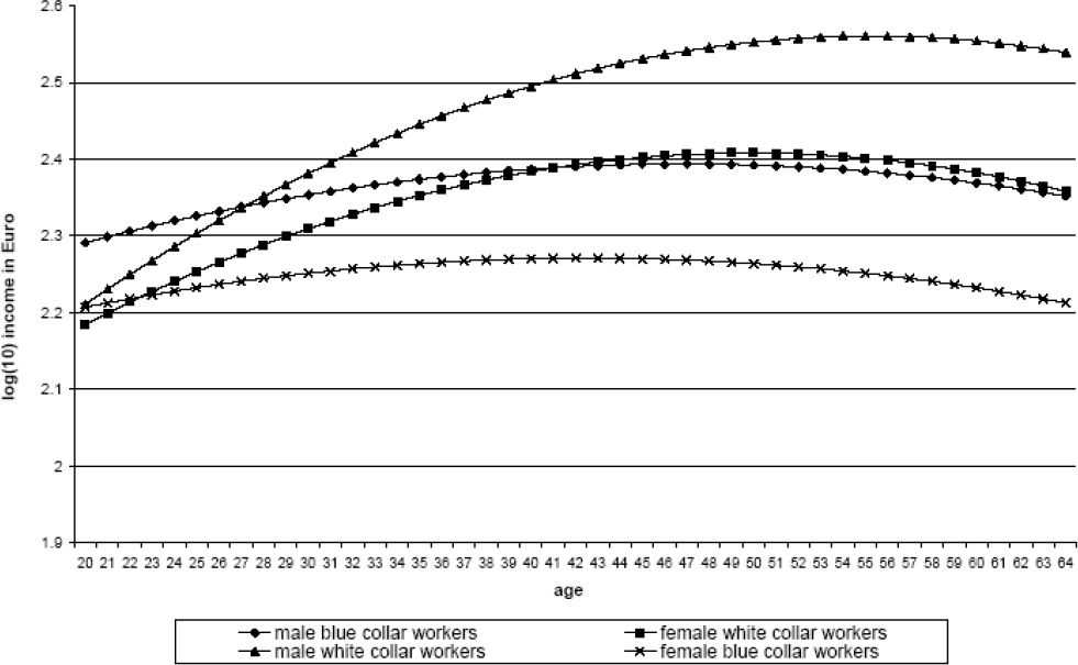
Now all that is left do is to estimate a wage profile f(.), separately for each category of worker, which relates the wage per day of an individual in that category aged age to that of a 20 year old. This has been done using simple quadratic regression on wage data from the 3rd quarter of 1998, again using data source (3). Figure A2 contains the resulting wage profiles.
As might be expected, both male and female blue collar workers have a less steep wage profile than white collar workers. Furthermore, the wage per day of young male blue-collar workers is higher than that of white-collar workers, both male and female; and although the wage of female white-collar workers catches up rapidly at first, it only ends up slightly higher than that of male blue-collar workers from the age of 40 on.
To summarize, the growth of individual wages between two years, t and t + 1 (and, therefore, between age and age + 1) is determined by the growth rate of the macroeconomic wage wt (Figure A1), whereas the wage difference between two individuals of different age at t is determined by the relationships captured in Figure A2.
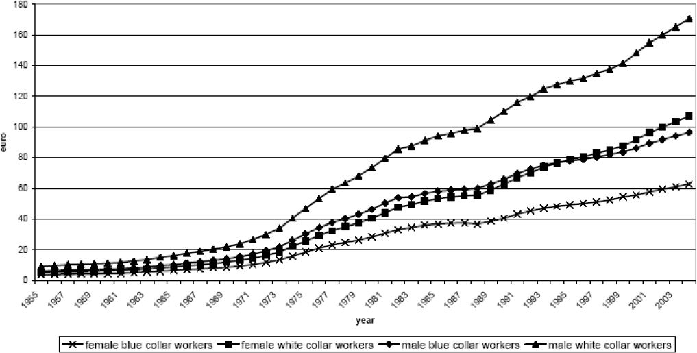
Wage per day for the categories of workers as a whole.

Logarithm of the gross wage per day as a function of age.
References
-
1
Pension Reform in Germany: The impact on Retirement Decisions. NBER Working Paper No 9913National Bureau of Economic Research.
-
2
Incentive effects of social security on labor force participation: Evidence in Germany and across EuropeJournal of Public Economics 78:25–29.
-
3
Databanken RSZ: “LATG-brochure” en “snelle ramingen”Databanken RSZ: “LATG-brochure” en “snelle ramingen”, mimeo General Directorate, ADDG(03) VB-KH/6450/9070, dossier 006/002, Brussels, Federal Planning Bureau, August4.
-
4
Databank RSZ-gecentraliseerdDatabank RSZ-gecentraliseerd, mimeo General Directorate ADDG(03)6476/VB-KH/9112, dossier 006/002, Brussels, Federal Planning Bureau, October22.
-
5
De Financiële Implicaties van Langer Werken: een MicroEconomisch Pensioen Model (MEP). Working Paper No 15/05Brussels: Federal Planning Bureau.
-
6
Micro-modeling of retirement in BelgiumIn: J. Gruber, D Wise, editors. Social Security Programs and Retirement around the world: Micro-estimation (1). Chicago: the University of Chicago Press. pp. 41–98.
-
7
The Retirement Effects of Old-age Pension and Early Retirement Schemes in OECD Countries. Economics Department Working Papers Nr. 370Paris: Organisation for Economic Co-operation and Development OECD.
-
8
Adequate and Sustainable Pensions – joint report by the Commission and the CouncilBrussels: European Commission, Directorate-General for Employment and Social Affairs, Unit E.2.
-
9
IntroductionIn: J. Gruber, D Wise, editors. Social Security Programs and Retirement around the world. Chicago: the University of Chicago Press. pp. 1–36.
-
10
IntroductionIn: J Gruber, D Wise, editors. Social Security Programs and Retirement around the world: micro-estimation. Chicago: the University of Chicago Press. pp. 1–41.
-
11
Bruto-lonen en Werk-gelegenheid: lange-termijnreeksenBruto-lonen en Werk-gelegenheid: lange-termijnreeksen, mimeo General Directorate ADDG(01) KH/6305/8719, Brussels, Federal Planning Bureau, July31.
-
12
Jaarlijks verslag van de Studiecommissie voor de vergrijzingJaarlijks verslag van de Studiecommissie voor de vergrijzing, Brussels, April.
- 13
-
14
Mathematische Demografie: Bevolkingsvooruitzichten 2000–2050 per arrondissementBrussels: Nationaal Instituut voor de Statistiek.
-
15
Het effect van wijzigingen in vervroegde uittredingsregelingen op de arbeidsparticipatie van oudere werknemersThe Netherlands: research rapport Center Applied Research for the Ministry of Social Affairs.
-
16
Labour Force Participation of Groups at the Margin of the Labour Market: Past and Future Trends and Policy Challenges. ECO/CPE/WP1(2003)Paris: Organisation for Economic Co-operation and Development OECD, Economics Department for Working Party No 1 on Macroeconomic and Structural Policy Analysis.
-
17
Praktijkboek Sociale Zekerheid voor de onderneming en de sociale adviseurBrussels: Ced.Samsom.
- 18
-
19
Simulatiemodellen: Instrumenten voor Sociaal economisch Onderzoek en BeleidTijdschrift voor Sociologie 26:137–153.
Article and author information
Author details
Acknowledgements
The author wishes to thank two anonymous referees for their helpful comments.
Publication history
- Version of Record published: December 31, 2007 (version 1)
Copyright
© 2007, Dekkers
This article is distributed under the terms of the Creative Commons Attribution License, which permits unrestricted use and redistribution provided that the original author and source are credited.