Simulating disease transmission dynamics at a multi-scale level
- University of Liverpool, United Kingdom
- World Health Organization, Switzerland
Abstract
We present a model of the global spread of a generic human infectious disease using a Monte Carlo micro-simulation with large-scale parallel-processing. This prototype has been constructed and tested on a model of the entire population of the British Isles. Typical results are presented. A microsimulation of this order of magnitude of population simulation has not been previously attained. Further, an efficiency assessment of processor usage indicates that extension to the global scale is feasible. We conclude that the flexible approach outlined provides the framework for a virtual laboratory capable of supporting public health policy making at a variety of spatial scales.
Introduction
Global disease
In recent years the focus of medicine in the developed world has been on chronic diseases related to behaviour or local physical environment, while the major causes of death in developing countries, however, remain infectious diseases (Morens et al., 2004). This rift in the global focus is counter-balanced by a fear of the emergence or re-emergence of novel infectious diseases and of the introduction of infectious diseases into regions in which immunity is low or non-existent. The current worry of a within-species strain of avian influenza is typical of the need to understand the patterns of global diseases, their emergence, spread (Galvani and May, 2005; Lloyd-Smith et al., 2005) and the mechanisms of transmission (Sattenspiel and Herring, 2003), and by those means also the potential value of alternative interventions (Chatterjee, 2005; Ferguson et al., 2005; Halloran and Longini, 2006; Longini et al., 2005). While some of the public fear of potential new global epidemics generated by news headlines is perhaps unfounded, the expert concern about between-species transmission is real, founded and consequential (Tran et al. 2004). The HIV-AIDS pandemic is an example for a contact-transmitted disease, while sudden acute respiratory syndrome (SARS) is an example of an air-borne disease, both diseases having made a major impact on the public horizon.
Human infectious diseases are defined here as those diseases in which most cases are contracted as a result of contact with an already infected person. The actual mechanism of transmission between humans varies between diseases (Anderson & May, 1991). Such mechanisms include: physical contact, sexual contact, airborne, waterborne, foodborne or vector-borne. These mechanisms are some of the most determining factors in understanding and modelling transmission. Specifically, infectious diseases transmitted through physical contact are wholly dependent on human behaviour, while vector-borne diseases require an understanding of life cycle and natural history of the vector (Hoshen & Morse, 2004). Waterborne and foodborne diseases (such as cholera) are usually modifiable in practice by improved hygiene and sanitation. In contrast, airborne diseases tend to be dependent solely upon close physical proximity, with transmission typically dependent upon human density, rather than upon ‘risky’ behaviours.
In the following we shall, for simplicity, focus on modelling airborne disease, although the approach outlined allows for more complex processes to be modelled.
Simulation approaches
Due to the practical and ethical difficulties of conducting large scale experimental research in infectious diseases, the modelling of transmission dynamics using analytical and computational simulations is both attractive and necessary. Analytical solutions are elegant and general and are widely used (Anderson & May, 1991). They allow the generalisation of results to different diseases under different conditions, through the exchange of parameter values or interaction elements. They may allow the extension of the model to large populations or large areas. They can typically serve to establish conditions for a steady-state solution of the prevalence and incidence of the disease, the increase in infection rate at a single location, or the spread of disease through an isotropic homogenous surrounding. While such a model may be conceived for a disease with limited stage dependence based on a homogeneous background, there are as yet no analytical solutions for the spatial and temporal spread of disease on an inhomogeneous plane. An analytical model allowing for individual stochastic variation seems to be unattainable. One solution to this shortcoming is the use of computer simulations.
Simulations allow the modeller to create a reduced representation of the complexities of reality, while leaving in place aspects deemed relevant, and to test their relevance by successive exclusions of model sections. Input data to the simulation may be based on observed data or on a limited characteristic representation. Most biological models consist of some measurable parameters which are determined by empirical data (Ferguson et al., 2005). The simulation outputs will typically be expressed in terms of data with both spatial and temporal dimensions. While the temporal aspect is inherent to transmission models, a spatial aspect is important for models which represent either the spread of new diseases or else spatial variation due to spatially-expressed local conditions. The ability to simulate in silico the progression of a disease thus forms the basis for a virtual laboratory, which replaces the natural laboratory of chronic diseases. This virtual laboratory allows the evaluation of interventions to be tested, by assessing their impacts upon infection rates.
In simulating disease there has been a tendency to choose deterministic models in which individuals are bound to become infected within a set time (Anderson & May, 1991). More recent elaborations of these models describes the probabilistic flow of individuals from one status to another (e.g. Ferguson et al. 2005). Such models, unless containing an elaborate lag structure, however, often neglect a proper representation of the time-course and allow individuals to develop an infectious status faster than biologically feasible. A more valid method is to create separate “human” objects, followed individually, with dynamics that approximate those of actual humans (Chen & Bokka, 2005). By dynamics we refer here to the ability of the in silico humans to move within the virtual world and interact with other virtual objects and with the process of disease. These virtual objects could include not only disease status but also individual characteristics, which may range from age and gender to genetic traits. As may be expected, this method will in general carry the computational cost of a large population structure in terms of both time and memory. In particular, to represent the behaviour of the human system at the early stages of an outbreak the size of the virtual population must be of the order of magnitude of the real population. Perhaps the closest work in this field to our own is that of Ferguson et al. (2005, 2006) and Longini et al. (2005), both of which focus on avian influenza. Both are experimenting with large scale simulations, and have conflicting predictions of the potential risk associated with an outbreak. However, neither is targeting the global simulation of disease spread.
Due to the stochastic aspect of infection patterns, only this kind of dynamic microsimulation model will be able to simulate the full set of population processes required. Unfortunately, to fully generate the probability distribution will, in general, require many runs and huge memory and data resources. The additional complication of spatial transmission makes such models too complex for single processor machines. As a result, until now such models either compromised their geographic dynamic aspect, and simulated discrete individual locations, or else simulated only relatively small populations, either by limiting themselves to small countries (such as Sweden – c.f. Holm et al., undated) or by scaling the population. The innovative use of parallel-processing techniques introduced in this paper allows for the simulation of the entire macroscopic population.
Development of hardware
Modern computing facilities, based on parallel computing, enable user access to very large scale processing and memory resources many thousands of times greater than that available on a single PC. These facilities are typically clusters of low cost PCs which may easily be supplemented modularly, or else may be time-shared using inactive machines. Suitable software packages are freely available to enable linking machines. Large programs which exploit many hundreds of processors may thus be run interactively, allowing rapid evaluation of results and comparison of various parameters settings.
High performance computing (HPC) based on parallel-processors cuts costs and provides access to groups which would otherwise not have the facilities. Parallel processing has been used for years in military and large-scale-management systems, in physics and chemistry academic research and various other fields. In biology, utilisation is sparse, and mainly focussed in bioinformatics. Social science simulations seem to not have taken this path yet. The Virtual Population Laboratory at the University of Liverpool seeks to take advantage of the availability of the local HPC facilities and to use these resources to perform micro-simulations of disease patterns on a multiprocessor computer system, in order to develop operational disease forecasts.
Materials and methods
In the work reported here we have simulated the spread of a contagious disease over the UK and the Republic of Ireland. We have used this simulation to evaluate the impact of some basic intervention strategies such as the closure of schools, which otherwise allow large-scale inter-household transmission between school-children. The primary purpose of the example presented, however, is simply to demonstrate the feasibility of micro-simulating large (tens of millions) populations.
Hardware and packages
The computing facility at the HPC centre at the Department of Physics, University of Liverpool has 940 nodes, each of which is a single core 3.06 gigahertz DELL PowerEdge 650 server PC, with 1gigabyte of Random Access Memory. This computer cluster, known as MAP2, has an effective performance of 1.2 terraflops. Thirty seven nodes were allocated to the present pilot project. In such a computer cluster, inter-processor communications can impose a significant communications overhead. The switch fabric used in MAP2 is Gbit Ethernet linked into a Force 10 E600 fully non-blocking switch (with no oversubscription) directly connected to each processing node. The hardware interface was provided by a front-end server remotely accessed using RedHat Linux version 9.0. Parallel-processing was enabled using message-passing interface protocol (MPI, implemented by MPICH (Gropp et al., 2006). Programming was in C/C++ as implemented by MPICH, with the code compiled under mpiCC and gcc.
Data structure
For the simulation of the UK population we utilised a subgroup of a global dataset we previously constructed. The data consist of a global population density map fitted to a Cartesian grid format, and are taken from Gridded Population of the World (GPW) (CIESIN/CIAT, 2005). The resolution of the GPW is 0.25% or approximately 27 km by 27 km at the equator. This dataset was divided into countries using ArcGIS 9 and the supplied country boundary map. The total population within each grid cell was then subdivided by age-group and sex using country-specific age-sex structures provided by United Nations (2005). The resulting grid-based populations, disaggregated by age and sex, are adequate for the proof-of-concept model reported here. An obvious future refinement would be to use more detailed maps and census data where possible, although inter-country differences would necessitate additional work on data harmonization before the result could be used as the input to a global model.
The gridded population outlined above gives us a global structure of virtual “towns” (populated grid cells, each of approximately 27 × 27 km, depending upon location relative to the equator). These towns are further subdivided into grids of 1000 by 1000 buildings or “houses”, each sized approximately 27 m by 27 m. For each town we also created classrooms or “schools” (number of schools = 1/30 of the number of children < 15 years), workplaces (number of workplaces = 1/6 of the total adult population) and homes (number of homes = 1/3 of adult population). These three groups (houses, workplaces, homes) are placed at random in the grid and may overlap. Not all locations need be occupied and many areas are uninhabitable (sea for instance). To provide a simple but functional model of the British Isles, the choice of house size, along with the definition of schools, workplaces and homes, were fixed ad hoc. In a fully operational model the size of each element could be altered to better reflect the known demographic / geographic reality, although for running a global model using currently available technology we would not recommend using a spatial grid with a size below that of a standard room (approximately 3m × 3m).
Having created a spatial framework, each towns is populated by creating virtual “humans”, objects (agents) possessing day and night locations, personal schedules (at this time only time of starting and ending work), age, sex and disease status. The total population and the age-sex structure of each town’s population is already known. These adults and children are randomly allocated to homes within that town (i.e. to ‘houses’ designated as being available for occupation). Adults and children in each home are then also randomly allocated to, respectively, workplaces and schools within the town, a small proportion being randomly allocated to a workplace or school in an adjacent town. Each individual is also assigned a disease status from one of a sequence of possible states: susceptible, infected, latent (non-infectious), infectious and immune. The lengths of the latent and immune stages are variable and can be modified by disease type, as can the infection and clearance rates. In a typical model run the vast majority of individuals are assigned an initial disease status of susceptible, with only a few individuals, in a few selected towns, being randomly allocated the disease status of infected.
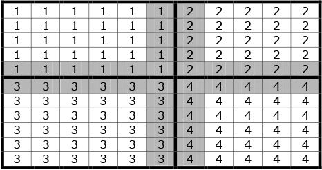
Because a full model for a large land mass is typically beyond the capacity of a single processor, the total surface area is subdivided into “regions” each controlled by a single processor. For simplicity the mesh of houses towns and regions is currently a Cartesian grid, but there exists no intrinsic computational reason that this geometry could not be refined (as is usual within finite element analysis) to further optimize the performance of the model. Adjacent processors overlap by two rows of towns, which are duplicated on each. This is a computational artefact to allow transfer across region boundaries, with each inner row belonging to the self region, and the outer row being attributed principally to the remote region. This is illustrated in Figure 1, in which the cells represent ‘towns’ and the numbers within each cell represent the controlling processor. Regions are denoted by a thicker borderline. The shaded cells (towns) are those which are mirrored in adjacent processors.

Example of the grid structure of regions, towns and overlaps.
Algorithms
Population dynamics
The time evolution of the system is modelled in time or clock steps. Our investigation used a clock step representing 15 minutes, or 1/96 of a day.
Further refinements of the system allowing for more detailed simulation of human behaviour could use a faster clock speed. Currently at each clock step the following processes occur.
The first process takes place in each town independently. People move from night to day location at the start of their scheduled day, and vice versa at its end. In the case of quarantine or curfew, part of the movement may be limited. For example, schools may be closed, in which case children remain in their homes (night location) during the day.
A second tier process is the movement of population between adjacent towns. This may be of two kinds: daily commuters who work in one town and live in the next, corresponding to suburban homes; and migrants who move away for a sustained period, and as such may be treated as residents at their new location. In the commuting case, both local home and remote workplace are stored for the individual. At the end of each time step the population of each town located on the border of two regions is copied across to its mirror image in the adjacent region.
A third tier process is long-distance movement, defined as movement to a non-adjacent town. In the present setting this movement may be either within a region or between regions. In this process there is no memory of initial location and the new member person is attributed a new home and workplace. This is clearly artificial and further work would allow for the same person to return home after an extended long distance trip. Unlike the first and second tier processes above, long-distance movement is only implemented once per day.
Rates for commuting and migrations are proportional to the size of the remote town (which prevents short term net population flux) and are controlled by a parameter which reflects local conditions (such as socioeconomic status). These parameters may be replaced by data on travel where available. This process would render the model more accurate, but would not otherwise affect the functionality of the model provided in this paper.
Disease dynamics
The starting point for the model is the introduction of one or more cases of a disease into the population. At each subsequent time step the following procedure is followed.
The number of infectious people in each house is counted.
The entire population list is traversed. For each person a new infection state is evaluated. The per-step probability for an uninfected person to become infected by a single infected person is designated α. Assuming infection by different infectious people being independent, the probability of being infected by n people in a house is calculated by the joint probability of not being infected by any of them. Thus a susceptible person may become infected (latent) if residing in the same house with n infectious persons with the probability 1−(1−α)n. Latent patients progress one stage towards infectious status, with the last stage representing their becoming infectious. Infectious patients become not infectious and immune with clearance probability β, whilst immune persons make one step towards becoming susceptible, with the last step being susceptibility. An implementation of a non-exponential distribution of the duration of infection may be introduced when applicable.
The number of infectious persons is summed for each town, for each region (processor) and globally. As individual move between towns or regions, their individual disease status is transferred with them.
Evaluation of output
In this paper we evaluate two issues: the feasibility of the model structure for larger scale models; and ways of splitting the total investigation area into regions. To fulfil these twin goals we ran the program using differing configurations of processors and differing methods of grouping towns into regions. The total number of processors used ranged from 4 to 36. Two alternative methods were used to group the grid cells (towns) required to represent the British Isles into regions. The first involved grouping towns into lateral slices, the second involved grouping towns longitudinally and latitudinally. The subdivisions were geared to test the scalability of the program, the limitations regarding numbers of processors, the minimum time for a run and the use of alternative processor architectures to reduce data-swapping. For this testing we used either a 24 by 24 grid subdivided as described in Table 1, or a 36 by 36 grid subdivided as described in Table 2. In both tables the first column reports the total number of processors used in each configuration, whilst the second (third) column gives the number of towns that each processor controls in the x (y) direction. In all cases the model was run for 30 virtual days and the real world time was monitored.
Alternative 24 × 24 grid configurations.
| Total regions (processors) |
Shape of region | Simulation Time (seconds) |
|
|---|---|---|---|
| Towns along X-length | Towns along Y-length | ||
| 1 | 24 | 24 | 921 |
| 2 | 12 | 24 | 878 |
| 2 | 24 | 12 | 835 |
| 3 | 24 | 8 | 815 |
| 4 | 24 | 6 | 826 |
| 4 | 12 | 12 | 791 |
| 4 | 6 | 24 | 722 |
| 6 | 24 | 4 | 595 |
| 8 | 24 | 3 | 460 |
| 12 | 24 | 2 | 356 |
| 24 | 8 | 3 | 444 |
| 24 | 6 | 4 | 427 |
| 24 | 12 | 2 | 359 |
| 24 | 24 | 1 | 281 |
| 24 | 1 | 24 | 211 |
| 36 | 8 | 2 | 345 |
| 36 | 4 | 4 | 328 |
| 36 | 2 | 8 | 296 |
Alternative 36 × 36 grid configurations.
| Total regions (processors) |
Shape of region | |
|---|---|---|
| Towns along X-length | Towns along Y-length | |
| 4 | 18 | 18 |
| 9 | 12 | 12 |
| 36 | 1 | 36 |
| 36 | 3 | 12 |
| 36 | 2 | 18 |
| 27 | 4 | 12 |
| 18 | 6 | 12 |
| 12 | 9 | 12 |
Spatially, the grids share a common origin to the North West of England. Hence the 24 × 24 grid covers most of Ireland, Western Scotland and parts of Wales (population ~5 million); whilst the 36 × 36 grid covers Scotland, Ireland, Wales and northern England, including Manchester, Leeds and Birmingham (population ~20 million). To further test model scalability, a final set of model runs involved a 48 × 48 grid covering the entire British Isles with the exception of the Kent lowlands (total population ~70 million).
Results
Time course
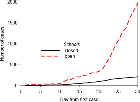
One typical time course for the development is presented here (Figure 2). It represents the number of cases of an airborne respiratory disease, after the introduction of a single infectious case in the English Midlands. The latency was set to 3 days, as was the post-clearance immunity (though larger times showed no significant difference). One hundredth of adults commuted between towns daily, and there were no long distance movements. The rate of infection of a susceptible person when within the house of an infectious person was 0.9. The red line represents the number of cases without public health intervention, and the black line the number when a policy of closed schools is implemented.

A typical time course for disease spread (origin = Midlands).
Statistics
The incorporation of the stochastic elements of disease transmission requires multiple runs. The results presented in Figure 3 display the mean, median and first and third quartiles. Because the data are not normally distributed this representation is preferable to the use of the standard deviation or standard error. We note that an important feature of this model is that a frequency distribution is a natural output of the model.
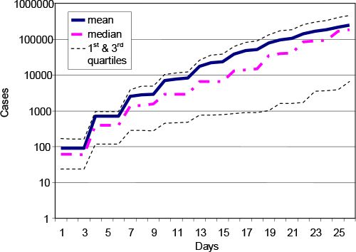
Time course for 20 runs, assuming 1% of adults commute daily and schools are kept open.
Spatial patterns
The spread of the infected cases among the general population is fairly isotropic. The largest numbers are, as expected, in the metropolitan areas, which afterwards serve as sources for subsequent transmission. This is because the high density regions have a higher commuter in-migration rate, there are more people to be infected within a populous town and there are more people to exit the town carrying the disease. In Figure 4 we present three snapshots of a series of 30 daily pictures of the distribution of a rapidly spreading disease.
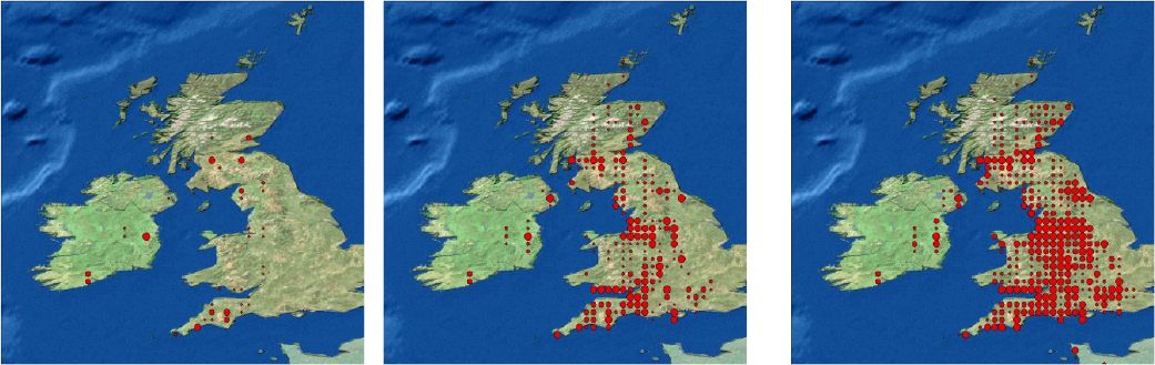
Spatial distribution of cases after 3, 19 and 25 days for a highly infectious disease, allowing for long distance transmission. The size of the dot represents the number of cases at the grid point.
Note: Disease outbreak was seeded randomly in three initial centres.
Speed and numbers of nodes
The practicality of such a model relies on the speed required to perform a run. The typical run times for the 48 × 48 grid model covering almost the entire British Isles required about 100s/run using 36 nodes (processors). Assuming that 100 runs are performed to obtain a useful distribution this means an effective run-time of ~104s (3hrs) is required to simulate the daily commuting, migration and disease spread behaviour of a population of ~70 million over a virtual time-period of 30 days (2880 time steps, each representing 15 minutes of elapsed time). However, a complex interaction exists between regional topology, the number of processors involved in the simulation and total execution time. This is discussed further below.
Discussion
Model validity and future refinements
Despite the simplicity of our current ‘proof-of-concept’ model, some of the results generated already match well-known reports. Our model is able to create a representation of nationwide transmission (Figure 4). This spread does not occur in all cases, nor in all runs. In fact, the probability of self-containment of the disease decreases with the number of persons already infectious, in line with expectation (Mills et al., 2006). Closure of schools, as depicted in Figure 2, has also been shown elsewhere to be an effective means for limiting transmission (Heymann et al., 2004; Monto, 2006), although more so in rural situations, as urban children tend to fraternise in extra-school settings. Leisure activity has yet to be implemented in our model; if it had been we would expect our results to reflect this additional observation.
Additional improvements planned for the future include enhanced modelling of variable person mobility tendencies, which should peak at around middle age, with elderly persons moving much more infrequently. Diurnal movements will also be modified to allow for visiting additional places and at additional times. At the same time transport modelling will introduced to allow for en route infection, for example in buses, trains and aircraft (Brockmann et al., 2006; Hufnagel et al., 2004). Similarly, the model will be revised to implement disease-induced absenteeism from work.
Model scalability
The principal value of our model’s structure is its modularity and conceptual simplicity, allowing the model to be scaled up, in principle, to a global model. In such scaling up a primary constraint on model execution time is the region with maximal population. The reason for this is that, in our model structure, there is a pause at the end of each time step to allow the swapping of information between regions, principally the mirroring of towns located on a regional border to the adjacent regional processor. As a result the processor dealing with the region containing the highest population, and which therefore takes the longest to complete its computational task, is the one which will dictate the pace of the simulation. This is illustrated by results produced using the 36 by 36 grid (Figure 5a). As the number of processors increases, the maximal population of each region falls, thereby reducing the overall simulation time. This suggests that scaling the model from a national (British Isles) to global scale will simply require more processors.

Changes in MPI usage efficiency in response to grid size and processor nodes.
However, the story is not quite that simple. The mirroring process has associated communication overheads, with the overhead being proportional to the size of the population that has to be mirrored. When sub-dividing a less densely populated region across multiple processors, the gains in computation power more than out-weigh the slight increase in communications overhead entailed. On the other hand, when sub-dividing a densely populated region (e.g. London), the increase in communications overhead, with far greater volumes of population having to be mirrored between regions, can potentially off-set any gain in computing power. This is the cause of the diminishing returns shown at work in Figure 5b, based upon results from model runs using a 24 × 24 grid. Communication overheads are also affected by the arrangement of towns within a region into rows and columns. This is demonstrated visually in Figure 5b where, for the same number of processors, multiple points are plotted, indicating the range of run times that can arise depending upon the precise arrangement of towns within regions. (The specific regional configurations associated with each run time are shown in Table 1.)
Several lessons can be drawn from Figure 5. First, provided region size is large enough to allow the modelling of major metropolitan areas on one processor, communication overheads do not play a limiting factor in model run times. Rather, scaling the model up from national to global coverage is simply a case of increasing the number of processors used. To simulate the world we estimate approximately 1000–10000 processors would be necessary, already within the range of some existing regional computer cluster facilities. Second, the way in which populations are distributed across processors is important. We are currently developing an algorithm that will partition the total population into equally populated regions, while allowing for boundary interfaces to be managed simply. This will sharply reduce the maximal processing speed-limit caused by highly dense metropolitan centres such as London. Of course, in a more sophisticated microsimulation, with an increase in the amount of data per individual, the limitations imposed by communication overheads would be more severe, but the lessons above still apply. In any case, we believe efficient packing of the data should limit this additional effect.
The generic nature of the model
The principal goal of this project was to demonstrate the feasibility of large-scale microsimulation of disease dynamics using high performance cluster computing resources. Using currently available technology, the model structure proposed has been shown to be able to run a microsimulation of the entire UK population, and, by extrapolation (using additional processors), of a continent or the world. The model at this stage is a transmission model, with a simple “black box” of transmission dynamics. This black box can be adapted to different forms of directly transmitted disease. Microsimulation modelling particularly suits the stochastic dynamics observed at the early stage of a potentially global disease, as both transmission and clearance from the individual are probabilistic, and at the individual level may cause survival or eradication of the virulent strain. On the other hand, microsimulation only seems appropriate for modelling the spread of a disease from a region with moderate prevalence to other regions when the travel rate is low. When a large proportion of the population are mobile, less computationally demanding deterministic methods are sufficient.
After the epidemic simulations reported here and elsewhere (Ferguson 2005, 6), perhaps the largest dynamic microsimulation reported in print is SVERIGE (Holm et al., undated), which models the lifepaths of c. 9 million separate individuals. Of course, in comparison to SVERIGE epidemic simulations are limited in scope, modelling only transmissible disease. Nor do these models base themselves on the type of detailed data-structure which is available to the SVERIGE group, due to the extensive data-collection system of the Swedish government, and its availability to researchers. Such personal data are rarely available in other countries, either because the data do not exist (as in developing countries) or due to regulation of data (as in most other developed countries). In addition, SVERIGE places its basic human focus on the family, a term missing in the reported epidemic microsimulations, which focus instead on the health of individuals living in households. However, these differences are not intrinsic to the simulation structure outlined in this paper, but rather are a result of our own distinct modelling goals. According to modelling need either the ‘home’ or ‘individual’ objects in our model could be treated instead as a ‘family’. Similarly, additional personal characteristics and behaviours could be factored in, either readily (e.g. earnings and taxes; family formation and dissolution; localised mortality and fertility rates), or after some additional work (e.g. matching of employees with local, regional and national job vacancies). Even the uniform grid currently utilised in our model can be simply transformed, via topological mapping, to cater for existing non-grid-based administrative geographies, tying in directly with existing census data sources without affecting model functionality (c.f. Ferguson et al., 2005). The real difference between SVERIGE and our model is simply that of scale. Our model demonstrates how the modelled population of a geographically detailed microsimulation can be scaled up through the computationally efficient subdivision of spatial units across multiple processors.
Conclusion
Potential for use in decision making
The model presented appears to bear promise as a tool for the future evaluation of alternative interventions in the control of infectious diseases. We emphasize that this computational framework could support multiple diseases and virtual populations differentiated by parameters values. While the current underlying disease transmission model would remain transparent, the addition of extra layers of environmental and clinical data would allow the study of sophisticated phenomena with increasing spatial and temporal resolution. Thus the model is not static and inflexible, but open to a process of successive refinement. Naturally such development would require access to international epidemiological data.
The model is, of course, strictly dependent on the assumptions regarding the black box of the individual disease pattern. Indeed, the variation of the parameter values, and some of the interaction assumptions of the population reflect the difference between diseases, and hence the potential virulence (Anderson & May, 1991; Lloyd-Smith et al., 2005; Weiss & McMichael, 2004). Inevitably, the insertion of inappropriate parameter values will necessarily cause incorrect evaluation of the impact of interventions. A corollary of this, from a policy point of view, is that if adjusting a parameter yields radically varying results this indicates a gross sensitivity which can act as an indicator to where further study of the disease or the intervention should be pursued.
Feasibility of extension
The program is modular, requiring only the definition of the simulation boundaries. The population is readily structured for the simulation, and the program can, with minimal changes, be used for any size region, although the partitioning to regions must be performed efficiently. We are currently investigating the use of meshing algorithms to refine this partitioning and the effect of these meshes on performance. However the current algorithm is adequate.
At present the model has been developed and has demonstrated the capacity to model disease transmission in the UK and Ireland. The main limitation on the model is the number of processors available on the local prototype cluster. A cluster of ~1000 processors (or cores) (1 terraflop) would permit the modelling of Europe and of order 10,000 the modelling of the world (10–100 terraflops). With efficient partitioning of populations across processors the authors believe these numbers could be reduced by an order of magnitude, making global modelling accessible to typical current national or regional computing clusters. For example the UK North-West Science Grid (http://www.nw-grid.ac.uk) will provide up to about 4000 cores capable of running this global model by 2007.
We believe that the generic modelling approach presented in this paper provides a first step towards the creation of a novel tool for use by the international microsimulation community. We also hope, more broadly, that it provides a challenge to this same community to revisit the issue of the computational limits to microsimulation modelling. As we have demonstrated, microsimulation models no longer have to confine themselves to use of a single computing processor.
References
- 1
- 2
- 3
-
4
Stochastic modeling of nonlinear epidemiologyJournal of Theoretical Biology 234:455–70.
-
5
Gridded Population of the World, Version 3, Center for International Earth Science Information Network and Centro Internacional de Agricultura TropicalPalisades, New York: Columbia University.
-
6
Strategies for containing an emerging influenza pandemic in Southeast AsiaNature 437:209–14.
- 7
- 8
-
9
MPICH2 User’s Guide, version version 1.0.4Argonne National Laboratory.
-
10
Public health. Community studies for vaccinating schoolchildren against influenzaScience 311:615–6.
-
11
Influence of school closure on the incidence of viral respiratory diseases among children and on health care utilizationPediatric Infectious Diseases Journal 23:675–7.
-
12
The SVERIGE spatial microsimulation model – content, validation and example applicationsSpatial Modelling Centre, Universitet Umea.
- 13
-
14
Forecast and control of epidemics in a globalized worldProceedings of the National Academy of Science U S A 101:15124–9.
-
15
Superspreading and the effect of individual variation on disease emergenceNature 438:355–9.
- 16
-
17
Pandemic influenza: Risk of multiple introductions and the need to prepare for themPublic Library of Science Medicine 3:e135.
-
18
Vaccines and antiviral drugs in pandemic preparednessEmerging Infectious Diseases 12:55–60.
- 19
-
20
Simulating the effect of quarantine on the spread of the 1918–19 flu in central CanadaBulletin of Mathematical Biology 65:1–26.
-
21
Avian influenza A (H5N1) in 10 patients in VietnamNew England Journal of Medicine 350:1179–88.
-
22
World Population and Prospects: The 2004 RevisionNew York: United Nations Population Division.
-
23
Social and environmental risk factors in the emergence of infectious diseasesNature Medicine 10:S70–6.
Article and author information
Author details
Acknowledgements
The MAP2 DELL Cluster is part of the North-West Grid, which is funded by the North-West Development Agency, the CCLRC Daresbury Laboratory and the Universities of Lancaster, Liverpool and Manchester. MBH was supported by the North-West Grid.
Publication history
- Version of Record published: December 31, 2007 (version 1)
Copyright
© 2007, Hoshen et al.
This article is distributed under the terms of the Creative Commons Attribution License, which permits unrestricted use and redistribution provided that the original author and source are credited.