FiFoSiM – An integrated tax benefit microsimulation and CGE model for Germany

The aim of this paper is to describe FiFoSiM, the integrated tax benefit microsimulation and computable general equilibrium (CGE) model of the Center for Public Economics (CPE) at the University of Cologne (Finanzwissenschaftliches Forschungsinstitut an der Universität zu Köln (FiFo)). Fuller documentation is provided by a number of unpublished working papers including Peichl and Schaefer (2006), which is a shortened English version of a more detailed German description (Fuest et al., 2005b), all available from the project website (www.cpe-colgone.de). FiFoSiM consists of three main parts. The first part is a static tax benefit microsimulation module. The second part adds a behavioural component to the model: an econometrically estimated labour supply model. The third module is a CGE model which allows the user of FiFoSiM to assess the global economic effects of policy measures. Two specific innovations distinguish FiFoSiM from other tax benefit microsimulation models for which peer-reviewed accounts are available: first, the simultaneous use of two databases for the tax benefit module and second, the linkage of the tax benefit model with a CGE model. The paper is notable also for bringing into one place discussions of a range of ‘standard’ techniques, including statistical matching, imputation, and implementation of both CGE and discrete choice household labour supply models. Hence, in addition to presenting the methodological innovations already alluded to, it is hoped that this paper will serve as a jumping-off point for others involved in planning, constructing and refining similar models.

The basic module of FiFoSiM is a static microsimulation model for the German tax and benefit system using income tax and household survey micro data. In the last few years a number of tax-benefit microsimulation models have been developed for Germany. (For example, Peichl, 2005; Wagenhals, 2004.) Most of these models use either GSOEP or FAST as a database. FAST is a micro datafile from the German federal income tax statistics containing the relevant income tax data of nearly 3 million households in Germany. GSOEP, the German Socio-Economic Panel, is a representative panel study of private households in Germany. The approach of FiFoSiM is innovative in that it creates a dual database drawing upon both micro datasets. The simultaneous use of both databases allows for the imputation of missing values or variables in either dataset using techniques of statistical matching.

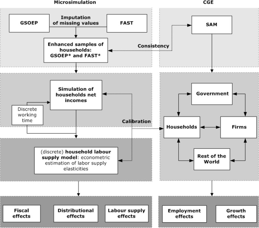
Figure 1 shows the basic setup of FiFoSiM. The tax benefit module follows several steps. First, the database is updated to the ‘current’ year using static ageing techniques. Cases are reweighted to allow for projected changes in global structural variables, whilst a differentiated adjustment is implemented for different income components of the households. (Gupta and Kapur (2000) provide a more detailed overview of static ageing techniques.) Second, we simulate the current tax system using the modified data. The result of this simulation provides the benchmark for different reform scenarios, which are also modelled using the updated database.

Figure 1

Download asset Open asset

In order to model the tax and transfer system, FiFoSiM computes individual tax payments for each case in the sample considering gross incomes and deductions in detail. The individual results are multiplied by the individual sample weights to extrapolate the fiscal effects of the reform with respect to the whole population. After simulating the tax payments and the received benefits we can compute the disposable income for each household. Based on these household net incomes we estimate the distributional and the labour supply effects of the analysed tax reforms. For the econometric estimation of labour supply elasticities, we apply a discrete choice household labour supply model. Furthermore, FiFoSiM contains a CGE module for the estimation of growth and employment effects, which is linked to the tax benefit module. This interaction allows for a better calibration of the model parameters and a more accurate estimation of the various effects of reform proposals.

The organisation of this paper is as follows. Section 2 describes (the creation of) the dual database of FiFoSiM, while Section 3 describes the tax benefit module. Section 4 contains a description of the labour supply model, while Section 5 describes the CGE module. In Section 6, several applications of FiFoSiM are presented and some developments planned for the further improvement of FiFoSiM are outlined.

A specific feature of FiFoSiM is the simultaneous use of two micro databases, allowing for the imputation of missing values or variables in both datasets. Due to the time lags between data collection and data availability, the two datasets have to be updated to represent the German economy in the period of analysis. The two data sources, and the matching and ageing processes applied to them, are described in detail in the following. The use of a third database in the CGE module is described separately (Section 5).

2.3 Creating the dual database

One special feature of FiFoSiM is the creation and usage of a dual database. To be more precise, FiFoSiM actually consists of two tax benefit microsimulation models. The first one is based on administrative tax data (FAST), the second on household survey data (GSOEP). The main reason for using a dual database instead of having only one merged database is the huge difference in the number of observations (3 million vs. 30,000). Furthermore, both databases have shortcomings, as described in the previous sections. Technically, cases in the two datasets could be matched with each other through the use of unique personal identifiers. In Germany, however, there are legal barriers to such a solution. Instead, FiFoSiM relies upon statistical matching. In this way information from one database is used to impute missing values or variables in the second dataset and vice versa. The end result is that FiFoSiM actually consists of two enhanced datasets, which allows for a better analysis of tax benefit reforms than using either original dataset alone.

There exist several principal ways for statistically matching datasets and imputing missing values. Rässler (2002) gives an introduction to statistical matching procedures and imputation techniques, as well as an overview of the vast literature and software packages that exist. D’Orazio et al. (2006) provide an alternative introduction to well-known techniques originally developed during the 1970s (c.f. Okner, 1972; Radner et al. 1980), whilst more recent developments in imputation methods are outlined by Rubin (1987) and Little and Rubin (1987). Finally, Cohen (1991) provides a survey of statistical matching applied in other fields of research. However, although statistical matching and missing value imputation are well established approaches, as far as we know no peer-reviewed microsimulation model has previously adopted the dual database solution of FiFoSiM. The remainder of this Section (2.3) reports the methods of imputation and statistical matching used by FiFoSiM. The problem of database updating is then considered in Section 2.4, before the strengths and limitations of this dual database approach are returned to in Section 2.5.

2.3.1 Imputation of missing values

When faced with missing values in one variable the best, but of course most expensive, way to impute the missing values would be to collect further information on the missing data. But even this solution cannot compensate for shortcomings in historic datasets. An alternative would be to delete (or at least omit) cases containing missing values. However, this procedure would lead to biased estimations if the people with missing values share the same characteristics. Instead, as we review below, a number of statistical approaches offer better solutions.

In general, the imputation of missing values stands for replacing missing data with “plausible values” Schafer (1997: 1). Let K be a variable from a dataset A with i non-missing values N = (n₁,n₂,...,n_i) and j missing values M = (m₁,m₂,...,m_j): K = (N,M) = (n₁,n₂,...,n_i, m₁,m₂,...,m_j), and O = (O₁,O₂,...) a vector of (other) variables without missing values. At the same time, but for a different dataset, B, let H be the same variable as K and P the same as O. A range of solutions to finding ‘plausible’ values of M exist.

Mean substitution

In this approach, the missing values M in variable K are either substituted by the mean of the non missing values N:

(1) $\widehat{K}=(N,\overline{N})=(n_1,n_2,\dots ,n_i,\overline{n},\overline{n},\overline{n}),$

or they are substituted by the mean of the same variable H from a different dataset B:

(2) $\widehat{K}=(N,\overline{H})=(n_1,n_2,\dots ,n_i,\overline{h},\overline{h},\overline{h}).$

If the missing values can be attributed to some specific subgroups, then the missing values for each subgroup are replaced by the mean of each subgroup from the non missing values of either K or H.

Mean substitution reduces the variance of K and should therefore be an option of last resort, only considered if other approaches outlined below are not applicable. The latter could be the case if, for example, there is no correlation between K and any other variable. Mean substitution is used in FiFoSiM if a reform proposal includes the taxation of a so far untaxed activity, the distribution of which is not captured in an existing micro dataset.

Regression

In the regression approach, a function for the estimation of the missing values is constructed by regressing N, the non-missing values of K on other (non missing) variables O:

(3) $N=O\beta .$

Or, as in the case of mean substitution, the similar variable of non-missing values of H from a different dataset B are regressed upon P, the other variable present in B.

(4) $H=P\beta .$

These regression coefficients β are then used to predict the missing values. Often a stochastic random value û is added to the prediction of the missing values M to allow for more variation:

(5) $\widehat{M}=O\widehat{\beta }+\widehat{u}$

or

(6) $\widehat{M}=P\widehat{\beta }+\widehat{u}$

These estimates $\widehat{M}$ are then used to replace the missing values M:

(7) $\widehat{K}=(N,\widehat{M})$

In FiFoSiM this approach is mainly used for variables originating in the FAST98 database. Most of the missing values in FAST are due to anonymisation; their plausible values can be restricted to specific intervals given the additional information captured by the other non-missing variables. For categorical variables logistic regressions are often undertaken. Greene (2003) provides a good introduction to the different regression techniques available.

Multiple imputation

In the multiple imputation approach, multiple values for each missing value are simulated. That is, the missing data is filled in q times using the regression approach, each time, with different draws from the distribution of the stochastic error term to generate q complete data sets. These multiple datasets are generated to better reflect the variation in the estimates and the uncertainty in the imputation procedure itself:

(8) ${\tilde{M}}^r=({{\tilde{M}}^r}_1,{{\tilde{M}}^r}_2,\dots ,{{\tilde{M}}^r}_j),\text{\hspace{0.17em}for\hspace{0.17em} }r=\text{1\hspace{0.17em}to\hspace{0.17em}}q.$

Hence it is possible to compute the variance, and confidence interval or P-value of the missing value.

The average of these estimate values,

(9) $\widehat{M}=\frac{1}{q}{\displaystyle \sum _{r=1}^q{\tilde{M}}^r},$

provides the estimator for the relevant missing values and is used to replace the missing values, M, in the original dataset.

This approach is used in FiFoSiM for most of the GSOEP variables containing missing values. The relatively small number of cases in the GSOEP allows the use of several simulation runs for the imputation in a few minutes, whereas for the FAST data this method takes noticeably longer.

2.3.2 Statistical matching

Ideally, one would like to find perfect matches all of the time. This is possible if one has access to variables which uniquely identify an individual, such as name, address, date of birth, social security number. In reality, for reasons of respondent confidentiality, researchers are not allowed to gain access to raw micro data that includes this information. Instead, access is provided to anonymised datasets in which uniquely identifying characteristics have been removed or modified. As a result, exact matching is not possible. We therefore have to use methods of statistical matching to match close (instead of exact) observations that share a set of common characteristics.

The idea of combining two existing datasets to create a joint dataset was developed during the 1970s (c.f. Okner, 1972; Radner, 1980; Cohen, 1991). The general principle is to merge two (or more) separate databases through the matching of the individual cases. This matching is performed on common variables that exist in both databases (for example gender, age and income). The idea underlying this statistical matching approach is that if two people have a lot of things in common (like for example age, sex, income, marital status, number of children), then they are likely to have other characteristics (like for example expenses) in common.

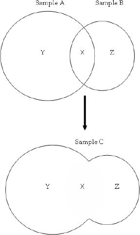
Figure 2 illustrates this basic idea of statistical matching. To put it more analytically, following Sutherland et al. (2002), we have three sets of variables X,Y,Z and two samples A = (X,Y) and B = (X,Z). X are the common variables in both samples (for example gender, age and income), Y and Z are sample specific (for example hourly wages and working hours from GSOEP, special tax deductions from FAST). We can now create a new, joint sample C = (X,Y,Z) by merging a recipient sample (let’s say A) with observations from a donor sample (b) with exact (or close) values of X. In doing so, one assumes that the conditional Independence Assumption (CIA) holds: conditional on X, Y and Z are independent. In other words, if we know X, Y(Z) contains no additional information about Z(Y) (Sims, 1972a, b, 1974). This assumption can “in practice […] rarely be checked” (Sutherland, Taylor and Gomulka (2002: 519). However, if the CIA does not hold, Paass (1986) observes that one can still use methods of statistical matching if the relationship between Y and Z can be estimated from other sources and incorporated into the matching process.

Figure 2

Download asset Open asset

As outlined below, statistical matching of two databases can be tackled using regression or data fusion methods. Note that which sample is chosen as the recipient, and which as the donor, depends upon the particular matching problem.

Regression

In the regression approach, the specific variable from the donor dataset Z is regressed on the vector of common variables X:

(10) $Z=X\beta .$

Often a stochastic random value V is added to the prediction to allow for more variation:

(11) $\widehat{Z}=X\widehat{\beta }+\widehat{v}.$

The estimated coefficients β from the donor dataset are then used to predict the values of Z in the joint dataset:

(12) $C=\left(X,Y,\widehat{Z}(\beta )\right)$

A strong correlation between X and Z is important for a successful merging. This approach is rather easy to perform, but it has the drawback that information in terms of variation is lost in the second dataset.

Data fusion

There are two main approaches to data fusion: nearest neighbour and propensity score matching. The general idea of both approaches is the same; they differ in detail only in the first step.

The first step in the nearest neighbour approach is to weight and norm the common variables, whereas in the propensity score approach, the first step is to estimate a propensity score, defined as the conditional probability of treatment given (the common) background variables (Rosenbaum and Rubin, 1983). In other words, the propensity score is used as a predictor of the probability of being in the treatment group versus being in the control group. In our case, an observation is in the treatment (control) group if it comes from the recipient (donor) sample.

To estimate the propensity score, a dummy variable I is introduced into the pooled dataset D, containing the common variables X from both samples A and B, with a value of 1 if the observation is from the recipient dataset and 0 if it is from the donor dataset:

(13) $I=\left\{\begin{array}{l}\text{1 if observation is from the recipient file}\hfill \\ \text{0 if observation is from the donor file}\hfill \end{array}\right.$

Then a logit or probit estimation of the probability of the observation being from the recipient sample (that is of the dummy indicator variable being 1), conditional on the common variables X, is calculated:

(14) $P(I=1|X)=f(X\beta )$

The function f(Xβ) is called the propensity score and indicates the probability of the observation belonging to the treatment group (the recipient sample).

The second step is similar for both approaches. The distance between the observations from both datasets is computed using a distance function (for a discussion of which, see Cohen, 1991). In the nearest neighbour case, the distance is based on the weighted common variables. In the propensity score case, the distance is based on the estimates for the propensity scores, which can be interpreted as some sort of implicit weighting function.

In the third step, the joint database C = (X,Y,Z) is created by merging the observations from the two datasets A and B with the minimal distance between them. Three ways of merging are possible: one observation from the donor dataset is merged to one observation from the recipient dataset (one-to-one merging); or one observation from the donor dataset is merged to multiple observations from the recipient dataset (one-to-n merging); or multiple observations from the donor dataset are merged to multiple observation from the recipient dataset (n-to-m merging).

In FiFoSiM the type of statistical matching used is determined by the number of observations (3 million vs. 30,000). In general, information from the smaller GSOEP dataset is matched to the FAST data using the regression approach. FAST information is merged to GSOEP data using propensity score matching.

In this section, the modelling of the German tax benefit system is described. As the Germany tax benefit system is very complex, we focus on the major parts of the model in this description. A more detailed description can be found in the German version of this documentation (Fuest et al., 2005b).

A key element of FiFoSiM is the analysis of the behavioural responses (labour supply effects) induced by the different tax reform scenarios simulated. Surveys of different kinds of labour supply models, including continuous time models, are provided by Blundell and MaCurdy (1999), Creedy et al. (2002) and Hausman (1985). A discrete choice model has the advantage of offering the possibility of modelling nonlinear budget constraints (e.g. Van Soest, 1995; MaCurdy et al., 1990). Furthermore, a discrete choice between distinct categories of working time seems to us to be more realistic than a continuum of choices because of working time regulations. Following Van Soest (1995), therefore, we apply a discrete choice household labour supply model, assuming that the household’s head and his/her partner jointly maximise a household utility function involving the net income and leisure time of both partners.

More formally, household i (i = 1,...,N) can choose between a finite number (j = 1,...,J) of combinations (y_ij,lm_ij,lf_ij), where y_ij is the net income, lm_ij the leisure of the husband and lf_ij the leisure of the wife of household i in combination j. Based on our data we choose three working time categories for men (unemployed, employed, overtime) and five for women (unemployed, employed, overtime and two part time categories).

Following Christensen et al. (1971) we model the following translog household utility function

where x = (ln y_ij, ln lm_ij, ln lf_ij)' is the vector of the natural logs of the arguments of the utility function. The elements of x enter the utility function in linear (coefficients ß = (ß₁, ß₂, ß₃)’), in quadratic and gross terms (coefficients A_(3x3) = (a_ij)). Using control variables z_p (p = 1,...,P), we control for observed heterogeneity in household preferences by defining the parameters ß_m and α_mn

where m,n = 1,2,3.

In FiFoSiM we use control variables for age, children, region and nationality, which are interacted with the leisure terms in the utility function because variables without variation across alternatives drop out of the estimation in the conditional logit model (Train, 2003).

Following McFadden (1973) and his concept of random utility maximisation (McFadden, 1981; 1985; Greene, 2003) we then add a stochastic error term ε_ij for unobserved factors to the household utility function:

Assuming joint maximisation of the households utility function implies that household i chooses category k if the utility index of category k exceeds the utility index of any other category / ∈ {1,...,J}\{k}, if U_ik > U_il. This discrete choice modelling of the labour supply decision uses the probability of i to choose k relative to any other alternative l:

Assuming that ε_ij are independently and identically distributed across all categories j according to a Gumbel (extreme value) distribution, the difference in the utility index between any two categories follows a logistic distribution. This distributional assumption implies that the probability of choosing alternative k ∈ {1,...,J} for household i can be described by a conditional logit model (McFadden, 1973; Greene (2003) and Train (2003) provide textbook presentations):

For the maximum likelihood estimation of the coefficients we assume that the hourly wage is constant across the working hour categories and does not depend on the actual working time. This assumption is common in the literature on structural discrete choice household labour supply models (Van Soest and Das, 2001). For unemployed people we estimate their (possible) hourly wages by using the Heckman correction for sample selection (Heckman, 1976, 1979). A detailed description of these estimations can be found in Fuest et al. (2005b). The household’s net incomes for each working time category are then computed in the tax benefit module of FiFoSiM.

The labour supply module of FiFoSiM is based on GSOEP data, which is enriched by information taken from the FAST data as described in Section 2.3. The sample of tax units is then categorised into six groups according to their assumed labour supply behaviour. We distinguish fully flexible couple households (both spouses are flexible), two types of partially flexible couple households (only the male or the female spouse has a flexible labour supply), flexible female and flexible male single households, and inflexible households. We assume that a person is not flexible in his/her labour supply, meaning he or she has an inelastic labour supply, if a person is

• younger than 16 or older than 65 years of age

• in education or military service

• receiving old-age or disability pensions

• self-employed or civil servant.

Every other employed or unemployed person is assumed to have an elastic labour supply. We distinguish between flexible and inflexible persons because the labour supply decision of those assumed to be inflexible (e.g. pensioners, students) is supposed to be based on a different leisure consumption decision (or at least with a different weighting of the relevant determinants) than that of those working full time.

The tax benefit and labour supply modules of FiFoSiM account only for the household side of the economy. The computable general equilibrium (cGE) module allows us to simulate the overall economic effects of policy changes including the production side. As a result the effects on labour demand, employment and economic growth as well as wage and price levels can be assessed. In this section of the paper, drawing upon Bergs and Peichl (2008), we describe the static CGE module in FiFoSiM, programmed in GAMS/MPSGE (Brooke et al., 1998; Rutherford, 1999), which models a small open economy with 12 sectors and one representative household. For a more general introduction to CGE modelling see Shoven and Whalley (1984,1992) or Kehoe and Kehoe (1994). Although the utility of the CGE module presented here as a stand-alone model is rather limited, in combination with the tax-benefit and labour supply modules, the resulting model, FiFoSiM, becomes a powerful tool. This is illustrated in Section 6, which also outlines some further refinements planned for the CGE module.

5.1 The model

5.1.1 Households

The representative household in the CGE model maximises a nested Constant Elasticity of Substitution (CES) utility function as illustrated in Figure 3.

Figure 3

Download asset Open asset

The household first chooses between aggregated consumption (including leisure) today, Q, or in the future, S. The result of this optimisation is the savings supply. The present consumption leisure (or labour leisure) decision then takes place. The household maximises a CES utility function U(C,F) choosing between consumption C and leisure F:

(22) $U(C,F)={\left[{(1-\beta )}^{\frac{1}{{\sigma }_{C,F}}}{C}^{{\rho }_{C,F}}+{\beta }^{\frac{1}{{\sigma }_{C,F}}}{F}^{{\rho }_{C,F}}\right]}^{\frac{1}{{\rho }_{C,F}}}$

where ß is the value share, ρ the degree of substitutability and σ_C,F = ρ_C,F − 1/ρ_C,F the elasticity of substitution between consumption and leisure.

The budget constraint is:

(23) $p^{C}C=\omega (1-t^l)(E-F)+r(1-t^k)K+{\overline{T}}_{LS},$

where p^C is the commodity price, w the gross wage, t^l the tax rate on labour income, E the time endowment, r the interest rate, t^k tax rate on capital income and K the capital endowment. Consumption p^CC is financed by labour income w(1−t^l)(E−F), capital income r(1−t^k)K and the lump sum transfer, T̅_LS, that ensures revenue neutrality. Optimising Equation (22) subject to Equation (23) yields the demand functions for goods and leisure. From the latter we calculate the labour supply of the household. As outlined, the CGE module models only one type of labour. It is recognised that this rather strong assumption limits the expressiveness of the household side of the model even more, and is a part of the model for which future refinement is planned (see Section 6).

5.1.2 Firms

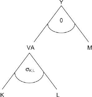
A representative firm produces a homogenous output in each production sector according to a nested CES production function. Figure 4 provides an overview of the nesting structure used in FiFoSiM.

Figure 4

Download asset Open asset

At the top level of the nest, aggregate value added, VA, is combined in fixed proportions, via a Leontief production function, with a material composite, M. M consists of intermediate inputs with fixed coefficients, whereas VA consists of labour, L, and capital, K. The CGE module allows for sector-specific wages and capital costs (although the latter is rarely used) depending on the context of the simulated reform. The optimisation problem at the top level of the nest, in each sector i, can be written as:

(24) $Y_i=\min \left[\frac{1}{a_{0i}}{f}_i(L_i,K_i);\frac{M_{1i}}{a_{1i}};\dots ;\frac{M_{12i}}{a_{12i}}\right]$

In the second level of the nest, the following CES function is used:

(25) $f_i(L_i,K_i)={\left[{\alpha }_i,L_i^{\rho i},+,(,1,-,{\alpha }_i,),K_i^{\rho i}\right]}^{\frac{1}{{\rho }_i}}$

where σ_i = 1/(1−p_i) is the constant elasticity of substitution between labour and capital.

The flexible structure of the model allows for different levels of disaggregation ranging from 1 to 3 to 7 to 12 sectors.

5.1.3 Labour market

To account for imperfections in the German labour market, a minimum wage W_i^min is introduced as a lower bound for the flexible wages in each sector. The labour supply is therefore rationed:

(26) $L_i^S=(1-\mu )\ge L_i^D.$

The minimum wage for each sector is calibrated so that the benchmark represents the current unemployment level in Germany.

5.1.4 Government

The government provides public goods, G, which are financed by input taxes on labour and capital, t^l and t^k. A lump sum transfer to households completes the budget equation:

(27) $G+{\overline{T}}_{LS}=t^{l}wL+t^{k}rK.$

5.1.5 Foreign trade

Domestically produced goods are transformed through a constant Elasticity of Transformation function into specific goods for the domestic and the export market, respectively. By the small-open-economy assumption, export and import prices in foreign currency are not affected by the behaviour of the domestic economy. Analogously to the export side, we adopt the Armington assumption (Armington, 1969) of product heterogeneity for the import side. A CES function characterises the choice between imported and domestically produced varieties of the same good. The Armington good enters intermediate and final demand.

1. 1
   A theory of demand for products distinguished by place of production

   1. P Armington

   (1969)

   IMF Staff Papers 16:159–176.

   • Google Scholar
2. 2
   Dynamic Fiscal Policy

   1. A Auerbach
   2. L Kotlikoff

   (1987)

   Cambridge: Cambridge University Press.

   • Google Scholar
3. 3
   Projektbericht 1 zur forschungskooperation mikrosimulation mit dem Bundesministerium der Finanzen, Materialien des DIW Berlin, Nr 26

   1. S Bach
   2. E Schulz

   (2003)

   Fortschreibungs- und hochrechnungsrahmen für ein einkommen-steuer-simulationsmodell, Projektbericht 1 zur forschungskooperation mikrosimulation mit dem Bundesministerium der Finanzen, Materialien des DIW Berlin, Nr 26, Deutsches Institut für Wirtschaftsforschung, Berlin.

   • Google Scholar
4. 4
   Numerische Gleichgewichtsmodelle zur Analyse von Politikreformen

   1. C Bergs
   2. A Peichl

   (2008)

   Zeitschrift für Wirtschaftspolitik 57:1–26.

   • Google Scholar
5. 5
   Das familienrealsplitting als reformoption in der familienbesteuerung

   1. C Bergs
   2. C Fuest
   3. A Peichl

   et al. (2006)

   Wirtschaftsdienst 86:639–644.

   • Google Scholar
6. 6
   Reformoptionen der Familienbesteuerung - Aufkommens-, Verteilungs- und Arbeitsangebotseffekte

   1. C Bergs
   2. C Fuest
   3. A Peichl

   et al. (2007)

   1–27, Jahrbuch fur Wirtschaftswissenschaften, (Review of Economics), 58, 1.

   • Google Scholar
7. 7
   Labor supply: A review of alternative approaches

   1. R Blundell
   2. T MaCurdy

   (1999)

   In: O Ashenfelter, D Card, editors. Handbook of Labor Economics, 3A. North Holland: Amsterdam. pp. 1559–1695.

   • Google Scholar
8. 8
   Combining top-down and bottom-up in energy policy analysis: a decomposition approach. ZEW Discussion Paper No 06-007

   1. C Böhringer
   2. T Rutherford

   (2006)

   Combining top-down and bottom-up in energy policy analysis: a decomposition approach. ZEW Discussion Paper No 06-007, ftp://ftp.zew.de/pub/zew-docs/dp/dp06007.pdf, accessed 11 November 2008.

   • Google Scholar
9. 9
   Steuern, transfers und private haushalte. Eine mikroanalytische simulationsstudie der aufkommens- und verteilungswirkungen

   1. C Bork

   (2000)

   Peter Lang: Frankfurt am Main.

   • Google Scholar
10. 10
    Representative versus real households in the macro-economic modelling of inequality. DIAL Document de Travail DT/2003-10

    1. F Bourguignon
    2. A-S Robilliard
    3. S Robinson

    (2003)

    Paris: DIAL, Institut de Recherche pour le Developpement.

    • Google Scholar
11. 11
    GAMS - A users guide

    1. A Brooke
    2. D Kendrick
    3. A Meeraus

    et al. (1998)

    Washington, DC: GAMS Development Corporation.

    • Google Scholar
12. 12
    That elusive elasticity: A long-panel approach to estimating the capital-labor substitution elasticity. CESifo-Working Paper No. 1240

    1. RS Chirinko
    2. SM Fazzari
    3. AP Meyer

    (2004)

    Munich: CESifo, University of Munich.

    • Google Scholar
13. 13
    Conjugate duality and the transcendental logarithmic function

    1. L Christensen
    2. D Jorgenson
    3. L Lau

    (1971)

    Econometrica 39:255–256.

    • Google Scholar
14. 14
    Growth, distribution and poverty in Madagascar: learning from a microsimulation model in a general equilibrium framework. TMD Discussion Paper 61

    1. D Cogneau
    2. A-S Robilliard

    (2000)

    Washington, DC: International Food Policy Research Institute.

    • Google Scholar
15. 15
    Statistical matching and microsimulation models

    1. ML Cohen

    (1991)

    In: C F Citro, E A Hanushek, editors. Improving information for social policy decisions: the uses of microsimulation modelling, Vol II Technical Papers. Washington DC: National Academy Press. pp. 62–85.

    • Google Scholar
16. 16
    Doha scenarios, trade reforms, and poverty in the Philippines: A Computable General Equilibrium analysis. World Bank Policy Research Working Paper 3738

    1. CB Cororaton
    2. J Cockburn
    3. E Corong

    (2005)

    Washington, DC: Worldbank.

    • Google Scholar
17. 17
    Microsimulation Modelling of Taxation and the Labour Market: The Melbourne Institute Tax and Transfer Simulator

    1. J Creedy
    2. A Duncan
    3. M Harris

    et al. (2002)

    Cheltenham: Edward Elgar Publishing.

    • Google Scholar
18. 18
    Microsimulation, CGE and macro modelling for transition and developing economies

    1. J Davies

    (2004)

    Mimeo: University of Western Ontario.

    • Google Scholar
19. 19
    Statistical matching: Theory and practice

    1. M D’Orazio
    2. M DiZio
    3. M Scanu

    (2006)

    Statistical matching: Theory and practice, Wiley, New York.

    • Google Scholar
20. 20
    FiFo-Bericht

    1. C Fuest
    2. A Peichl
    3. T Schaefer

    (2005)

    Aufkommens-, Beschaftigungs- und Wachstumswirkungen einer Steuerreform nach dem Vorschlag von Mitschke, FiFo-Bericht, 05, FiFo Koeln, Universitat zu Köln.

    • Google Scholar
21. 21
    Dokumentation FiFoSiM: integriertes steuer-transfer-mikrosimulations-und CGE-modell. Finanzwissenschaftliche Diskussionsbeitrage Nr 05 - 03

    1. C Fuest
    2. A Peichl
    3. T Schaefer

    (2005b)

    FiFo Koeln: Universitat zu Köln.

    • Google Scholar
22. 22
    Aufkommens-, beschaftigungs- und wachstumswirkungen einer reform des steuer- und transfersystems nach dem Burgergeld-Vorschlag von Joachim Mitschke. FiFo-Bericht 08–2006

    1. C Fuest
    2. S Heilmann
    3. A Peichl

    et al. (2006)

    FiFo Koeln: Universitat zu Köln.

    • Google Scholar
23. 23
    Aufkommens-, beschaftigungs- und wachstumswirkungen einer steuerreform nach dem vorschlag von Mitschke

    1. C Fuest
    2. A Peichl
    3. T Schaefer

    (2007a)

    Baden-Baden: Nomos.

    • Google Scholar
24. 24
    Die Flat Tax: Wer gewinnt? Wer verliert? Eine empirische analyse fur Deutschland

    1. C Fuest
    2. A Peichl
    3. T Schaefer

    (2007b)

    Steuer und Wirtschaft 84:22–29.

    • Google Scholar
25. 25
    Fuhrt Steuervereinfachung zu einer “gerechteren” Einkommensverteilung? Eine empirische Analyse fur Deutschland

    1. C Fuest
    2. A Peichl
    3. T Schaefer

    (2007c)

    Perspektiven der Wirtschaftspolitik 8:20–37.

    • Google Scholar
26. 26
    Does tax simplification yield more equity and efficiency? An empirical analysis for Germany

    1. C Fuest
    2. A Peichl
    3. T Schaefer

    (2008a)

    CESifo Economic Studies 54:73–97.

    • Google Scholar
27. 27
    Is flat tax reform feasible in a grown-up democracy of Western Europe? A simulation study for Germany

    1. C Fuest
    2. A Peichl
    3. T Schaefer

    (2008)

    International Tax and Public Finance, forthcoming.

    • Google Scholar
28. 28
    Econometric analysis

    1. W Greene

    (2003)

    New Jersey: Prentice Hall.

    • Google Scholar
29. 29
    Microsimulation in government policy and forecasting

    1. A Gupta
    2. V Kapur

    (2000)

    Amsterdam: North-Holland.

    • Google Scholar
30. 30
    DTC - Desktop Compendium to the German Socio-Economic Panel Study (GSOEP)

    1. J Haisken-DeNew
    2. J Frick

    (2003)

    Berlin: Deutsches Institut für Wirtschaftsforschung.

    • Google Scholar
31. 31
    Taxes and labor supply

    1. J Hausman

    (1985)

    In: A Auerbach, M Feldstein, editors. Handbook of public economics. Amsterdam: North-Holland. pp. 213–263.

    • Google Scholar
32. 32
    The common structure of statistical models of truncation, sample selection and limited dependent variables and a simple estimator for such models

    1. J Heckman

    (1976)

    Annals of Economic and Social Measurement 5:475–492.

    • Google Scholar
33. 33
    Sample selection bias as a specification error

    1. J Heckman

    (1979)

    Econometrica 47:153–161.

    • Google Scholar
34. 34
    A primer on static applied general equilibrium models

    1. P Kehoe
    2. T Kehoe

    (1994)

    Federal Reserve Bank of Minneapolis Quarterly Review 18:2–16.

    • Google Scholar
35. 35
    Statistical analysis with missing data

    1. R Little
    2. D Rubin

    (1987)

    New York: John Wiley & Sons.

    • Google Scholar
36. 36
    Assessing empirical approaches for analyzing taxes and labor supply

    1. T MaCurdy
    2. D Green
    3. H Paarsch

    (1990)

    Journal of Human Resources 25:415–490.

    • Google Scholar
37. 37
    Frontiers in econometrics

    1. D McFadden

    (1973)

    105–142, Conditional logit analysis of qualitative choice behaviour, Frontiers in econometrics, New York, Academic Press.

    • Google Scholar
38. 38
    Econometric models of probabilistic choice

    1. D McFadden

    (1981)

    In: C Manski, D McFadden, editors. Structural analysis of discrete data and econometric applications. Cambridge: The MIT Press. pp. 198–272.

    • Google Scholar
39. 39
    Econometric analysis of qualitative response models

    1. D McFadden

    (1985)

    In: Z Griliches, M Intrilligator, editors. Handbook of econometrics. Amsterdam: Elsevier. pp. 1396–1456.

    • Google Scholar
40. 40
    ADJUST FOR WINDOWS - A program package to adjust microdata by the Minimum Information Loss Principle. FFB-Dokumentation No 9

    1. J Merz
    2. H Stolze
    3. S Imme

    (2001)

    Luneburg: Department of Economics and Social Sciences, University of Luneburg.

    • Google Scholar
41. 41
    De facto anonymised microdata file on income tax statistics 1998. FDZ-Arbeitspapier Nr 5

    1. J Merz
    2. D Vorgrimler
    3. M Zwick

    (2005)

    Wiesbaden: Destatis.

    • Google Scholar
42. 42
    Erneuerung des deutschen einkommensteuerrechts: gesetzestextentwurf undbegrundung

    1. J Mitschke

    (2004)

    Koln: Verlag Otto Schmidt.

    • Google Scholar
43. 43
    Measuring distributional effects of fiscal reforms. Finanzwissenschaftliche Diskussionsbeitrage Nr 06 - 09

    1. R Ochmann
    2. A Peichl

    (2006)

    FiFo Koeln: Universitat zu Köln.

    • Google Scholar
44. 44
    Constructing a new data base from existing microdata sets: the 1966 merge  file

    1. B Okner

    (1972)

    Annals of Economic and Social Measurement pp. 325–342.

    • Google Scholar
45. 45
    Statistical match: evaluation of existing procedures and improvements by using additional information

    1. G Paass

    (1986)

    In: G H Orcutt, H Quinke, editors. Microanalytic simulation models to support social and financial policy. Amsterdam: Elsevier Science. pp. 401–422.

    • Google Scholar
46. 46
    Die evaluation von steuerreformen durch simulationsmodelle. Finanzwissenschaftliche Diskussionsbeitrage Nr 05-01

    1. A Peichl

    (2005)

    FiFo Koeln: Universitat zu Köln.

    • Google Scholar
47. 47
    Documentation FiFoSiM: integrated tax benefit microsimulation and CGE model. Finanzwissenschaftliche Diskussionsbeitrage Nr 06 - 10

    1. A Peichl
    2. T Schaefer

    (2006)

    FiFo Koeln: Universitat zu Köln.

    • Google Scholar
48. 48
    Measuring richness and poverty - a micro data application to Germany and the EU-15. CPE discussion paper No 06-11

    1. A Peichl
    2. T Schaefer
    3. C Scheicher

    (2006)

    FiFo Koeln: Universitat zu Köln.

    • Google Scholar
49. 49
    Social accounting matrices a basis for planning

    1. G Pyatt
    2. J Round

    (1985)

    Washington DC: The World Bank.

    • Google Scholar
50. 50
    Erneuerung der stichprobe des ESt-,odells des Bundesministeriums der Finanzen auf basis der lohn- und einkommensteuerstatistik 1995. Technical Report, GMD - Forschungszentrum Informationstechnik GmbH

    1. H Quinke

    (2001)

    Erneuerung der stichprobe des ESt-,odells des Bundesministeriums der Finanzen auf basis der lohn- und einkommensteuerstatistik 1995. Technical Report, GMD - Forschungszentrum Informationstechnik GmbH, St. Augustin.

    • Google Scholar
51. 51
    Report on exact and statistical matching techniques. Statistical Policy Working Paper 5, Federal Committee on Statistical Methodology

    1. D Radner
    2. R Allen
    3. ME Gonzales

    et al. (1980)

    Washington, DC: Office of Federal Statistical Policy and Standards.

    • Google Scholar
52. 52
    Statistical Matching

    1. S Rässler

    (2002)

    New York: Springer.

    • Google Scholar
53. 53
    The central role of the propensity score in observational studies for causal effects

    1. PR Rosenbaum
    2. DB Rubin

    (1983)

    Biometrika 70:41–55.

    • Google Scholar
54. 54
    Multiple imputation for non-response in surveys

    1. D Rubin

    (1987)

    New York: John Wiley & Sons.

    • Google Scholar
55. 55
    Applied General Equilibrium modeling with MPSGE as a GAMS subsystem: an overview of the modeling framework and syntax

    1. T Rutherford

    (1999)

    Computational Economics 14:1–46.

    • Google Scholar
56. 56
    Poverty and income distribution in a CGE-Household micro-simulation model: Top-down/bottom up approach. Working Paper 03-43, CIRPEE Centre interuniversitaire sur le risque

    1. L Savard

    (2003)

    Montreal: les politiques economiques et l’emploi.

    • Google Scholar
57. 57
    Analysis of incomplete multivariate data

    1. J. L. Schafer

    (1997)

    London: Chapman & Hall.

    • Google Scholar
58. 58
    Bevolkerungsentwicklung und wirtschaft-swachstum - eine simulationsanalyse fur die Schweiz

    1. C Schmidt
    2. T Straubhaar

    (1996)

    Schweizerische Zeitschrift fur Volkswirtschaft und Statistik 132:395–414.

    • Google Scholar
59. 59
    Applied general equilibrium models of taxation and international trade: An introduction and survey

    1. J Shoven
    2. J Whalley

    (1984)

    Journal of Economic Literature 22:1007–1051.

    • Google Scholar
60. 60
    Applying General Equilibrium

    1. J Shoven
    2. J Whalley

    (1992)

    Cabmridge: Cambridge University Press.

    • Google Scholar
61. 61
    Comments

    1. CA Sims

    (1972a)

    Annals of Economic and Social Measurement 1:343–345.

    • Google Scholar
62. 62
    Rejoinder

    1. CA Sims

    (1972b)

    Annals of Economic and Social Measurement 1:355–357.

    • Google Scholar
63. 63
    Comment

    1. CA Sims

    (1974)

    Annals of Economic and Social Measurement 3:395–397.

    • Google Scholar
64. 64
    The German Socio-Economic Panel (GSOEP) after more than 15 years - overview

    1. SOEP Group

    (2001)

    Vierteljahrshefte zur Wirtschaftsforschung 70:7–14.

    • Google Scholar
65. 65
    Volkswirt-schaftliche gesamtrechnungen: input-output-rechnung. Fachserie 18, Reihe 2

    1. Statistisches Bundesamt

    (2005)

    Wiesbaden: Destatis.

    • Google Scholar
66. 66
    Combining household income and expenditure data in policy simulations

    1. H Sutherland
    2. R Taylor
    3. J Gomulka

    (2002)

    Review of Income and Wealth 48:517–536.

    • Google Scholar
67. 67
    Discrete choice models using simulation

    1. K Train

    (2003)

    Cambridge: Cambridge University Press.

    • Google Scholar
68. 68
    Structural models of family labor supply: a discrete choice approach

    1. A Van Soest

    (1995)

    Journal of Human Resources 30:63–88.

    • Google Scholar
69. 69
    Family labor supply and proposed tax reforms in the Netherlands

    1. A Van Soest
    2. M Das

    (2001)

    De Economist 149:191–218.

    • Google Scholar
70. 70
    Tax-benefit microsimulation models for Germany: a survey

    1. G Wagenhals

    (2004)

    IAW-Report / Institut fuer Angewandte Wirtschaftsforschung (Tubingen) 32:55–74.

    • Google Scholar
71. 71
    Armington elasticities and product diversity in the European Community: a comparative assessment of four countries. Working Paper

    1. H Welsch

    (2001)

    University of Oldenburg.

    • Google Scholar

Author details

1. Andreas Peichl

   IZA Bonn, ISER and University of Cologne, Germany

   For correspondence

   peichl@iza.org

2. Thilo Schaefer

   Center for Public Economics, University of Cologne, Germany

   For correspondence

   schaefer@fifo-koeln.de