Dynamic spatial microsimulation using the concept of GHOSTs
- University of Leeds, UK
Abstract
This paper presents a novel method of creating and updating geographical population microdata. In particular, it presents a prototype modelling technique which forms a component of the SimBritain modelling project. The paper first briefly discusses some of the key conceptual and practical issues involved in microsimulation, in particular highlighting the differences between spatial and aspatial microsimulation models. The paper then outlines a potential alternative to fully stochastic event-driven spatial dynamic microsimulation. This alternative uses longitudinal data to produce and project Generic Household Spaces Through Time (GHOSTs), all within a spatial modelling framework. To this end the paper first outlines how to derive GHOSTs from longitudinal data, then explains how the attributes of these GHOSTs can be projected forward in time.
1. Introduction
One key distinction between microsimulation models, rarely noted in the literature, is that between spatial and aspatial microsimulation. Microsimulation has a long history in economics which led to the acceptance of the microsimulation method as a standard tool for the evaluation of economic and social policy and in the analysis of tax-benefit options and in other areas of public policy (Falkingham & Lessof, 1992; Hancock & Sutherland, 1992; Harding, 1996a; Mitton et al., 2000; Sutherland and Piachaud, 2001). The standard non-geographical microsimulation models now rest upon solid foundations built-up through systematic research by economists over the last forty years. However, during that period geography has been persistently ignored by microsimulation researchers, for several reasons:
Lack of good quality geographical data: there were very few sources of geographical socio-economic data. Even today population microdata, which form the baseline datasets used by economic microsimulation models, lack small-area spatial coding
Computational intensity: the incorporation of geography into standard microsimulation models increases significantly the computational demand
Concerns with simulation accuracy
Belief that geography is not important
Unfamiliarity with geographical data and methods
Some of these problems have been recently tackled due to an accelerating growth in the volume, variety, power and sophistication of the computer-based tools and methods available to support urban and regional analysis and policy-making. Developments in hardware and software systems have enabled significant advances to be made in the storage, retrieval, processing and presentation of spatially referenced data. There has also been significant progress in the development of Geographical Information Systems (GIS) for socio-economic applications (see for instance Longley et al., 2005). Further, there has been an increasing availability of a wide range of new geographical data sources in both the public and private sectors and an increased power and portability of personal computers (Bertuglia et al., 1994; Birkin et al., 1996).
Recently many spatial models (such as spatial interaction models and location-allocation models) have been developed that have shed new light on patterns and flows within cities and regions. These models, when combined with relevant performance indicators, have been very useful in measuring the quality of life for residents in different localities (Bertuglia et al., 1994; Clarke & Wilson, 1994). However, relatively little is known about the interdependencies between household structure or type and their lifestyles, including the events they routinely participate in and hence their ability to raise and spend various types of income and wealth. The modelling of interdependencies requires a different level of urban and regional system representation.
In this context, spatial microsimulation offers a potentially powerful framework for policy analysis. Adding spatial detail to traditional microsimulation involves creating a microdata set, as well as using it. There are very few sources of geographically detailed microdata sets, so there is a need to create these datasets using static geographical microsimulation techniques. It is interesting to note at this stage that economists would probably not use the term microsimulation for the creation of a microdata set, whereas in geography, most of the effort in microsimulation models had been in constructing good quality geographically disagaggregated population microdata. Geographical microsimulation techniques involve the merging of census and survey data to simulate a population of individuals within households (for different geographical units), whose characteristics are as close to the real population as it is possible to estimate.
In contrast, dynamic microsimulation involves forecasting past changes forward to produce as best an estimate as possible of individual’s circumstances in the future (O’Donoghue et al., 2009; Holm et al., 1996; Mertz, 1991). Both static and dynamic microsimulation models are typically underpinned by probabilistic or deterministic rules (Williamson, 2007; Ballas et al., 2005a,b).
This paper presents one of the dynamic components of SimBritain, which is a spatial microsimulation model, aimed at generating and projecting small area microdata in Britain. The paper draws on and builds upon recent work (Ballas et al., 2005a, 2007) and is structured as follows. Section 2 briefly reviews the aims and objectives of SimBritain and describes the method that it uses to generate small area microdata. Section 3 presents a novel method of updating the survey microdata and also describes a regression framework for the projection of continuous and non-continuous variables. Section 4 offers some concluding comments
2. The SimBritain project
At the root of SimBritain lies a relatively simple idea: that by using information from a relatively small number of people – for example from a sample or panel survey – and combining it with unrelated information from an extensive large-scale enumeration – such as the decennial Census of Population – it should be possible to add value to the survey microdata set and extrapolate its findings over both space and time (Ballas et al., 2005a). Much of the methodology underlying SimBritain is well-established. However it is important to recognise that all microsimulation models incorporate error. Even static spatial microsimulation models – those which model patterns or behaviours across space at one point in time – will not produce exact matches when tested against independent data. When these static models are made dynamic, projecting estimated variables into the future, the scope for error increases. In these circumstances it is important that the assumptions underlying the projections are both defensible and readily interpretable.
The basic methodology underlying the static spatial microsimulation component of SimBritain relies upon a technique known as iterative proportional fitting (Mosteller, 1968). SimBritain uses the iterative proportional fitting method in a reweighting fashion to generate an estimated small area microdata on the basis of the British Household Panel Survey (BHPS) and the Census of the UK population (Ballas et al., 2005). Specifically, we use samples of households from the BHPS and record their values in each of our six dimensions of interest – region, demography, household type, economic position, housing tenure and car ownership. We then decide upon the geographic area we are interested in modelling and the spatial units for which we wish to produce estimates. We then use the Census of Population to determine, for each spatial unit, the number of households falling into each category across our six dimensions of interest. A series of iterations is next performed, area by area, dimension by dimension. At each step, the weighted contribution of each BHPS household is adjusted so that, for a given spatial unit the sum of all household weights across a given dimension matches the corresponding Census total. Once a convergent set of weights emerges – typically after a dozen or fewer iterations – we have a list of household weights for each spatial unit, the weight being the number of times that household is represented in the simulated population for that area.
More information on this “deterministic reweighting” spatial microsimulation methodology is provided by Ballas et al. (2005a, 2007). This method represents an alternative to reweighting methods that involve random number generator reweighting approaches such as simulated annealing (first applied in such a context by Williamson et al., 1998). The method has also been used in combination with a small area population projection technique in order to estimate small area microdata for future points in time (by reweighting the survey data to the projected future dimension totals), thus adding an “implicitly dynamic” dimension (Ballas et al., 2005a). This modelling framework can also perhaps be described as a “dynamic model with static ageing” (for a detailed discussion of different types of microsimulation models see Harding, 1996b; O’Donoghue, 2001; Dekkers, 2003), and has been used to produce small area microdata for various points in time that can be used for policy analysis (Ballas et al., 2007). For a report on-going developments and refinements of the original method see Smith et al. (2009).
The key drawback of this framework is that it does not exploit the longitudinal nature of the BHPS. SimBritain was intended to eventually be a dynamic microsimulation of Britain that would fully exploit the panel nature of the survey data available to us to project existing trends into the future (i.e. to make use of the full set of year-on-year observations captured for each household, rather than simply exploiting a particular cross-sectional view of that household). However, two difficulties with this approach became apparent, following plausibility testing. First, the idea of allowing households to ‘move around’ SimBritain, constrained only by known and projected patterns of migration within the UK, proved impossible, primarily because of the lack of suitable migration data. A dynamic spatial microsimulation model, to work, has to incorporate migration, emigration, and immigration processes which can rapidly change the nature of small area. Second, the idea of ‘splicing’ household histories together, thereby extending for example a ten-year household record from the BHPS through to 2021, came up against fundamental difficulties of household definition, exacerbated by the effects of attrition upon panel surveys. The “splicing” idea was, to put it simply, to join the end (2001) of a household, in a household with similar characteristics in 1991 and use that to project forward to 2011.
In an attempt to overcome these difficulties, we developed the concept of a GHOST: a Generic Household Space through Time. Instead of making the household our centre of attention we concentrated instead upon the household spaces within which those households live. By moving away from the idea of ageing households over time and instead concentrating upon filling notional buildings with the sorts of households that typically inhabit them, we are able to use far more of the data in the panel survey, exchanging emphasis on consistency within a household’s history for plausibility in the history of the spaces which households inhabit. The following section discusses this process in some detail, developing a set of GHOSTs for Wales for the period 1991–2021. Section 4 then goes on to describe how these entities can be used for projection purposes.
3. Creating generic household spaces through time
3.1 Exploiting observed household histories
In order to exploit the panel nature of the BHPS, a method of creating household histories, which could be used to populate areas was developed. A BHPS life history database is relatively simple in concept: a row for each household and separate columns for each year for which data exists. A third dimension would contain whatever variables of interest are selected. When a household ceased to exist the row would cease and when a new household formed a new row would be created. Insofar as the composition of the country was changing, this would be reflected in the varying proportions of households of different types present in the database.
The task of creating these histories raises a critical question of definition. The standard definition of a household used in the BHPS and the Census is cross-sectional: the sharing of facilities at a given point in time. However, there are arguments about what constitutes a “longitudinal” household, given that the address or the composition of a household might change over time. As such, the question arises whether a household remains the same unit, given that individual household members may have left, due to death or moving out. By contrast new household members may enter the household over time, such as through a new birth or persons moving in.
One of the most extensive discussions of operational longitudinal household definition is provided by Ernst et al. (1984). In particular they concentrate on definitions in terms of what they term Same Householder, where a household is defined by reference to the head of household and Reciprocal Majority, where a household is defined by reference to the proportion of household members who are present in the household at time t and at time t + 1. The difficulties with the first approach relate to the definition of the head of household, which for most statistical purposes pays greater attention to economic activity than household continuity; and with the second that it can produce somewhat arbitrary results depending on the size of the household and the time period employed.
An alternative approach is provided by Frick and Haisken-DeNew (2001) using the German Socio-Economic Panel. They concentrate on change of address as the critical factor in identifying household dissolution and formation. Specifically, new households evolve when one or more individuals leave a pre-existing household and become resident at a new address. The drawback of this approach is that, as the authors recognise, “after several years a ‘household’ might consist of totally different persons than in the first wave”. However the identification of change of address as one element in a possible definition leads to a focus on the spatial dimension. Much of the literature reviewed had as its fundamental concern the dynamics of household formation and change. The perspective here is somewhat different. The concern is not so much with household processes per se, rather with their effects on the composition of local areas through time. If the emphasis is shifted from the household to the space in which that household lives, then a simpler approach can be adopted.
Specifically, the result is a database not of household histories, but rather of household space histories. As soon as the emphasis is shifted from the social to the physical the problem becomes much easier to conceptualise. What we are creating are thirty-year histories for a set of generic household spaces; while these are not identifiable dwellings, they can effectively be thought of as such, and over time they may see many changes in household composition. The resulting transition and new building, demolition and vacancy are also simpler to deal with than migration. The remainder of this section presents an illustrative example of using this method in Wales.
3.2 Creating GHOSTS for 1991–2000
The initial aim is to create a GHOST – a Generic HOusehold Space through Time – covering the period 1991–2000. It is generic, in that individual dwellings are not differentiated, but rather dwelling types; it concentrates on household spaces, defined as the physical spaces within which household units live; and it is considered through time (ten years in this case).
How are these GHOSTs created? The starting point is the BHPS 1991–2000. This contains information on all the households interviewed over that period of time. Unfortunately it does not identify the buildings in which these people live (while there are person identifiers and household identifiers there is no dwelling identifier). However it does contain information on various characteristics of the property (notably tenure, number of rooms and dwelling type) as well as the local authority area and whether individual members of the household have moved in the last year. Hence change or stability in dwelling may be inferred. On this basis it is possible to create a set of GHOSTs for Wales to cover the period 1991–2000.
3.2.1 Extracting histories of senior household members
The first step is to identify all senior household members who at any time during the period were interviewed in Wales. The household response for each year2 is established and a record is created for each household reference person3 or spouse4 or partner5 or other person recorded as head of household.6 For each of the above individuals interviewed a full history of their interviews, whether in Wales or not, and of the households to which they belonged at the time is extracted.
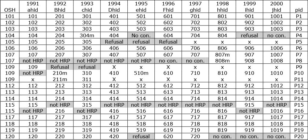
Figure 1 lists a sample of twenty such individuals together with their personal identifying number (pid) and their household identifying number (hid) at each wave. It also contains a newly derived variable called OSH or Original Sample Household. This is similar to the BHPS concept of OSM (Original Sample Member) in that every person interviewed in the BHPS is interviewed because they themselves were interviewed in the first wave (they are OSMs) or because they are currently in the same household as an OSM. The OSH is simply the first BHPS wave household identifier (BHPS variable ahid) for that OSM. When sorting out household histories the OSH is an invaluable indicator because it helps to disentangle some of the more complicated household histories (for example where members of families split off from original households only to rejoin at a later date) as well as clarifying apparent discontinuities in histories (for example where the family reference person changes between times despite no change in household composition, or where it is the result of the gain or loss of a member of another generation).

Individual interview histories for twenty Welsh members of the BHPS.
Notes: not HRP – not Household Reference Person; no con. – no contact; for guide to variable names see text.
Some of the cells in Figure 1 are shaded gray: this indicates either that although the individual was interviewed in the identified household, (s)he was not the head of household, household reference person (hrp) or spouse/partner at that time – eg pid P8 in wave a; or although an attempt was made to interview the person this was not successful – eg pid P9 in wave b. Where no entry appears in a cell this is because the individual did not appear on the interview schedules: either because the individual had been dropped by the BHPS (because of death, emigration, repeated refusal etc) – for example pid P9 from wave d onwards; or because (s)he was not an OSM and was not at that time living with an OSM – eg pid P11 in wave a. Changes of address are denoted by the suffix m.
The real value of these data will become apparent when household space histories are created, but Figure 1 also demonstrates some of the difficulties in assembling ‘simple’ household histories from panel data such as the BHPS. For example, OSH 115 did not move during the ten years of the study, but did contain varying numbers of people throughout that time. Furthermore two individuals were identified as household reference person at different times and with no apparent consistency: the parent (P15) was accorded that status in waves a, c and i, whereas the child (P16) was HRP in the remaining waves. By organising the data as shown in Figure 1 it becomes possible to identify the continuity which exists beneath apparent instability and underlines some of the potential pitfalls facing a mechanistic implementation of the Same Householder approach.
3.2.2 Constructing household space histories (1991–2000)
The next step is to convert these household interview histories into household space histories, a process which is achieved in two stages. As discussed above, a rigorous definition of household is not necessary: the ultimate aim is to create a history of each household space rather than household histories. However this methodology is effectively based upon the Same Householder approach described by Ernst et al. (1984), though with a (necessarily) flexible approach to the identification of the appropriate householder.
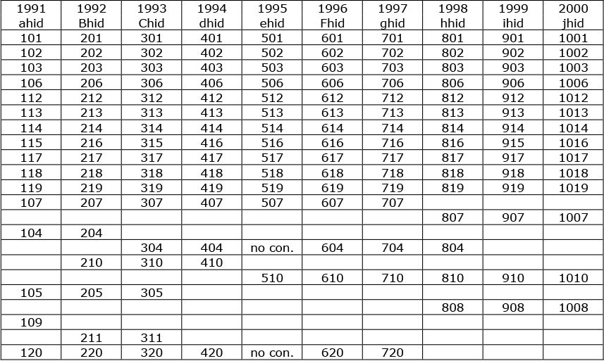
The first part of the process, represented in Figure 2, involves the separation and reordering of the various individual household histories identified above. First, any household which was identified in all waves of the study and which did not move address during those ten years is accorded a single row. Second, those household histories interrupted by changes of address are listed in consecutive rows with a new row for each new address. Finally come the remaining interview responses, with a row for each.

Individual household space histories derived from Figure 1.
Notes: no con. – no contact.
In terms of the twenty histories already identified in Figure 1 this produces: first, the eleven continuous household histories which did not involve a change of address (which in the case of OSH 115 involves the collapsing of two rows from Figure 1 to one in Figure 2); second, the sole example of a continuous history incorporating one change of address, producing two rows in Figure 2; and third, the seven remaining rows from Figure 1 which produce nine rows in Figure 2 because of the two changes of address affecting chid 304 and ehid 510 respectively. In terms of the entire Welsh subset of the BHPS, this approach distinguishes 140 households which were identified for ten years and which did not move during that time; 45 households (covering 102 rows) that have a full history but which did move; and the remaining interview responses which between them cover over 800 cells, equivalent to a further 80 ten-year household histories.
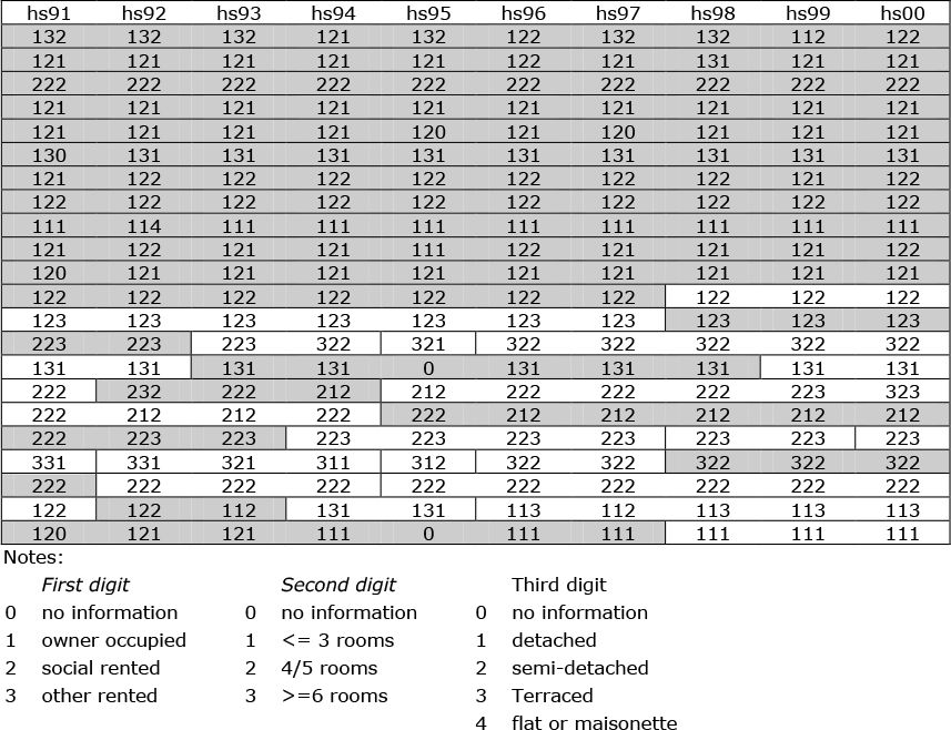
The second part of the process, represented in Figure 3, involves the compression and combination of information from the movers to create virtual histories for those household spaces which at the moment are represented by fragments. The first eleven rows of Figure 3 correspond to the first eleven rows of Figure 2, with household id information replaced by a code providing information on the dwelling in which the interview took. These rows are shaded gray to indicate the match with corresponding cells in Figure 2. It is worth noting that despite the fact that none of these households reported moving, there are not infrequent changes in household space information (which as the accompanying key explains, consist of information on tenure, dwelling size and type). Some of this will be real (changes in tenure or the building of extensions to homes, for example), but the remainder must reflect coding/response errors either in the household space information or else in the question on moves. For present purposes any apparent changes in household space information have been ignored and it has been assumed that the question on moves was correctly answered.

Generic household space histories derived from Figure 2.
The first seven cells of the twelfth row reflect the actual history of OSH 115, but as pid P7 moved between waves g and h (from a semi-detached to a terraced house) the virtual history for the semi is completed by the history of another household which moved into just such a dwelling in wave h. The history is virtual, in that the chances are infinitesimally small that the move was into the exact same dwelling, but there is a perfect match on tenure, dwelling type and size. The remainder of pid P7’s history appears in the next row, where it complements that of another Welsh household which lived in a terraced house until moving between waves g and h. The key issue here is that, although the chances of these histories applying to actual dwellings is unlikely, in aggregate they provide a plausible and unbiased estimate of all changes in an area.
Figure 3 provides five further examples of perfect matching on household space variables while the remaining four rows contain a close, but not perfect match. In the first such example in Figure 3 (row 14) an otherwise perfectly matched history is completed by the incorporation of one year’s data from a detached, rather than a semi-detached dwelling, in both cases privately rented with 4/5 rooms.
In terms of the entire Welsh subset of the BHPS, in addition to the 140 household spaces containing residents who did not move over the ten-year period there are: a further 66 rows which have been produced by perfect matching of household space descriptors; another 38 rows where the match is perfect on tenure but where there is a small difference in one of the other elements – a semi rather than a detached house or a small one rather than a medium-sized one; and 11 further rows where greater liberty has been taken with matching (but where two-thirds or more of the history for each row is consistent and whose inclusion helps to redress what would otherwise be a bias against rented tenures). This leaves some 140 cells (approximately 5% of the total valid interview record for Welsh households in the BHPS) which could not meet this standard. As a result of this flexible matching strategy the sample contains a changing profile of household spaces which (more or less) matches the changing profile of Welsh household spaces over the ten years in question, for all households in Wales.
From Figures 1 to 3 it should be clear how we have now created a representation of change in Wales with 255 household space histories covering the period 1991–2000. They are generic, in that 115 of them do not refer to the same physical dwelling, but each contains contemporaneous information.
3.3 Creating household ‘histories’ for 2001–2020
The next task is to project these histories through time: to project the 255 household space histories through to the year 2020. This is done in two stages. First the 255 GHOSTs for 1991–2000 are projected forward to 2010. The process is then repeated to project forwards another 10 years to 2020.
To project foward to 2010 the existing household space histories (from Figure 3) are duplicated and copied to their right thereby producing ten more columns (hs01-hs10). Then the pre-existing half of the table (columns hs91-hs00) is sorted by hs00 and the new half of the table is sorted by hs01. Within each category of hs00 and hs01, rows are further sorted by income so that the less affluent households appear first and the most affluent at the end of each respective category.
If there had been no change in the relative proportions of the different combinations of household space characteristics, there would be an identical match between hs00 and hs01 for each row in the table. In our Welsh sample all but thirty of the 255 rows are matched. Furthermore, because of the sorting by income, similar households (as well as household spaces) are matched.
Where there is no match between hs00 and hs01, the net was cast wider to allow for perfect matches between hs00 and hs02 or between hs99 and hs01 – this produces another 24 pairings. This still leaves six cases where no acceptable match was possible. This is inevitable given the changing profile of household spaces over time; indeed it is somewhat remarkable that as few as six out of 255 Welsh histories failed to pass the matching test. In these six cases the 2001–2010 history was produced by duplicating six records already matched – in each case using that record which perfectly matches on household space characteristics and most closely matches on income.
The second stage, taking the projections through to 2020, is achieved in analogous fashion. In total, 226 of the 255 rows are perfectly matched, 23 are matched on a best-fit basis, while another six histories were produced by duplication. This results in the 255 Welsh GHOSTs covering the period 1991–2020.
3.4 An illustrative history
As an example of what the generated household space histories mean in practice, consider the GHOST which had OSH 117 as its founder member. The household which lived in this smaller than average owner-occupied detached house in 1991 comprised a single pensioner who continued to live alone in the same house right through to 2000. The successor household for hs01 also comprised a single pensioner. However, within two years that pensioner had married and the couple continued to live in the same house for the next six years. No interview was achieved with the couple in wave h and hence new occupants were used to fill the generic household space. The new household comprised a married couple with their three children who provide the history for hs09 and hs10. The successor household for hs11 was similar to that in hs10, though with one fewer child. This situation persisted up to and including hs14, after which one of the parents left, leaving a single-parent household with two dependent children to live in the house up to and including hs20.
This example serves to illustrate the important characteristics of the approach. In this case a plausible history is generated for the household space in question. This will not always be the case, of course, with discontinuities concentrated at the changeover points between 2000/2001 and 2010/2011. Nevertheless many of the histories are credible and can be used to illustrate the nature of change affecting household spaces over time. Furthermore it should be noted that the primary use of GHOSTs is to provide plausible area estimates over time, the concomitant aggregation involved subsuming any inconsistencies in individual histories within the resultant aggregate spatial statistics.
4. Projecting changes in household attributes
While a methodology for populating household spaces over time is a necessary condition for the success of SimBritain, it is not sufficient. For this to be achieved we also need to provide a methodology for updating household attributes. This methodology falls into three parts.
At the moment, the household occupying a specific GHOST in, say, 2009 has the attributes of a real household interviewed in 1999. In a first step, therefore, the six known constraint variables for that household are used to predict the expected value of the variable of interest in 2009 for that ‘type’ of household (Section 4.1). In a second step, account is taken of the deviation of the actual from expected 1999 value to produce the 2009 projection (Section 4.2). Finally, account must be taken of projected compositional changes in local area populations (Section 4.3).
4.1 Projecting changes in expected household attribute values
For household attributes that are a time-invariant function of the external ‘compositional’ constraints, the reweighted GHOST estimates should provide plausible projections. However, an additional step is required to update the values of other household attributes, such as income or personal computer (PC) ownership, that are time-variant functions of the constraint variables. The approach outlined here adopts a general regression framework. To test this approach, it was decided to use existing data from the BHPS to model changes in two examples: household income (strictly speaking log of household income thereby compensating for income’s positively skewed distribution and minimising the biasing effect of extreme values) and personal computer (PC) ownership in Wales.
4.1.1 A regression framework for continuous variables
Initial modelling involved the specification of ten equations for the dependent variable (log(income)), one for each wave. This allowed not only the general level of the dependent variable to change over time, but also the pattern of dependence. However, it left the task of using the information from the ten models to project patterns into the future. In the course of trying to devise an appropriate methodology it became clear that an alternative, conceptually far simpler approach, was also available (Singer & Willett, 2003).
Consider the following set of simplified equations for the first three waves of the BHPS:
If an additional variable, WAVE, is specified then data from waves a, b and c can be combined within the same model as follows:
The advantage of this model is that it pools the data from the three waves, thereby increasing the reliability of the parameter estimates. The disadvantage is that the effect of each dependent variable is held constant over time. Thus whereas the first approach allows for changing patterns of relationship between dependent and independent variables (for example, the increasing gap in rates of PC ownership between car owners and non-car owners over the course of the ten waves), the second approach does not. The solution to this is to allow interaction effects between WAVE and each of the constraint variables in the model:
This gives two advantages: the increased reliability of parameter estimates resulting from the pooling of data together with a model that allows changing patterns of dependence upon the independent variables over time. The parameter estimates for modelling both log of household income and logit of pc ownership are shown in Table 1. In terms of the above equation, the coefficients a, b1, b2 b3 appear in the column main effect; while the coefficients b0, b11, b12, b13 appear in the column wave effect.
Parameter estimates for log (household income) and logit (PC ownership) together with example estimates for the period 1991–2020.
| INCOME | main effect | wave effect | Year 1991 | Income (£) 19,015 | PERSONAL COMPUTER OWNERSHIP | main effect | wave effect | Year 1991 | % with a PC 40 |
|---|---|---|---|---|---|---|---|---|---|
| intercept/wave | 9.10 | 0.014 | 1992 | 19,264 | intercept/wave | −1.51 | 0.125 | 1992 | 43 |
| London | 0.14 | 0.014 | 1993 | 19,516 | London | 0.24 | 0.021 | 1993 | 45 |
| SE | −0.04 | 0.018 | 1994 | 19,772 | SE | 0.07 | 0.006 | 1994 | 47 |
| SW | −0.19 | 0.022 | 1995 | 20,030 | SW | −0.10 | 0.013 | 1995 | 49 |
| Wales | 0.06 | −0.016 | 1996 | 20,292 | Wales | −0.16 | 0.022 | 1996 | 52 |
| E Anglia | −0.18 | 0.013 | 1997 | 20,558 | E Anglia | −0.24 | 0.014 | 1997 | 54 |
| E Midlands | −0.10 | 0.009 | 1998 | 20,827 | E Midlands | 0.16 | −0.032 | 1998 | 56 |
| W Midlands | −0.13 | 0.011 | 1999 | 21,099 | W Midlands | −0.23 | 0.010 | 1999 | 58 |
| NW | −0.07 | 0.020 | 2000 | 21,375 | NW | 0.10 | −0.016 | 2000 | 61 |
| Yorks & H | −0.11 | 0.012 | 2001 | 21,655 | Yorks & H | −0.11 | −0.007 | 2001 | 63 |
| North | −0.04 | 0.010 | 2002 | 21,939 | North | 0.18 | −0.032 | 2002 | 65 |
| Scotland | 0.00 | 0.000 | 2003 | 22,226 | Scotland | 0.09 | 0.001 | 2003 | 67 |
| No car | −0.76 | −0.002 | 2004 | 22,516 | No car | −0.41 | −0.037 | 2004 | 69 |
| One car | −0.36 | −0.001 | 2005 | 22,811 | One car | −0.04 | 0.006 | 2005 | 71 |
| Two+ cars | 0.00 | 0.000 | 2006 | 23,110 | Two+ cars | 0.45 | 0.031 | 2006 | 73 |
| Owned | 0.25 | 0.022 | 2007 | 23,412 | Owned | 0.20 | −0.001 | 2007 | 74 |
| Social rented | −0.03 | 0.030 | 2008 | 23,718 | Social rented | −0.28 | −0.024 | 2008 | 76 |
| Other rented | 0.00 | 0.000 | 2009 | 24,029 | Other rented | 0.08 | 0.025 | 2009 | 78 |
| High status | 0.63 | 0.007 | 2010 | 24,343 | High status | 0.48 | 0.024 | 2010 | 79 |
| Medium status | 0.40 | −0.001 | 2011 | 24,662 | Medium status | 0.31 | −0.015 | 2011 | 81 |
| Low status | 0.41 | 0.001 | 2012 | 24,984 | Low status | 0.10 | −0.013 | 2012 | 82 |
| Retired | −0.10 | 0.010 | 2013 | 25,311 | Retired | −0.95 | −0.008 | 2013 | 83 |
| Inactive | 0.00 | 0.000 | 2014 | 25,642 | Inactive | 0.06 | 0.012 | 2014 | 85 |
| Married | 0.39 | −0.005 | 2015 | 25,978 | Married | 0.18 | −0.011 | 2015 | 86 |
| Single parent | 0.13 | −0.004 | 2016 | 26,318 | Single parent | 0.16 | −0.006 | 2016 | 87 |
| Other | 0.00 | 0.000 | 2017 | 26,662 | Other | −0.34 | 0.017 | 2017 | 88 |
| No kids | 0.10 | −0.016 | 2018 | 27,011 | No kids | −0.71 | 0.036 | 2018 | 89 |
| One kid | 0.06 | −0.005 | 2019 | 27,364 | One kid | 0.17 | −0.001 | 2019 | 90 |
| Two+ kids | 0.00 | 0.000 | 2020 | 27,723 | Two+ kids | 0.54 | −0.035 | 2020 | 90 |
-
Notes: The estimated values are for a Welsh household with one car, living in an owner-occupied house, with a medium status head of household, married with two children.
As an example of how the estimated income of a household is calculated, consider a Welsh household in wave c (the third wave) with one car living in an owner-occupied house with a medium status head of household, married with two children. The intercept, six main effects, wave effect and six interaction terms are added (the wave effect and interaction terms multiplied by three because this is the third wave) and the resulting value exponentiated:
This value can be found in the third row of Table 1 where the estimated income of such a household is given for the period 1991–2020.
4.1.2 Regression framework for binary variables
Now consider the probability of the same household owning a PC in the fourth wave. Together with many of the topics of interest in the BHPS, computer ownership is a binary variable which is best modelled using logistic regression. In our example this is calculated as follows:
This value can be found in the fourth row of Table 1 where the estimated percentage of such households owning a computer is given for the period 1991–2020.
The utility of this modelling approach is best demonstrated by changing the selected characteristics of the chosen household. Thus if, for example, if this family lived not in Wales but in London, the probability would rise to 0.57; but if that London household was in social rented accommodation, the probability would fall back to 0.43.
4.2 Projecting changes in actual household attribute values
Using the above regression models provides a methodology for projecting changes in the expected value of variables of interest that encompasses both inflation and distributional change. However the actual 1999 value for a specific GHOST might well deviate significantly from the expected value for a household of that type. This reflects the important within-type heterogeneity captured in the original survey data. But the regression model will replace this actual 1999 value with an expected (average) value for 2009. How is the updating of the actual 1999 value to produce a projected 2009 value that retains the heterogeneity captured in the original survey?
In the case of a continuous variable, a relatively simple procedure can be used. If a particular variable, in this case household income, is defined as:
then
Following the example of the Welsh household, then if this specific household had an income of £15,000 in 1999, the projection for 2009 would be:
By applying multipliers specific to the type of household under consideration, inflation and distributional change are captured whilst at the same time maintaining within-group variability – i.e. the variability which exists between households which share the same values on all six constraint variables.
In the case of a binary variable, the issue is somewhat more problematic. Here the actual value for the selected household in 1999 can only be zero or one; multiplication of the former will have no effect while multiplication of the latter produces a meaningless number. What is required is not a multiplier but rather a mechanism whereby sufficient of the zeros are converted to ones (or vice versa depending upon the direction of the change). This is tackled by rescaling the probability rather than the outcome itself. In the example Welsh household discussed previously, its expected probability of owning a PC in 1999 is .58, rising to .78 in 2009. We now need a scaling factor that adjusts this probability of computer ownership in a way which reflects the fact that the 1999 outcome for this particular household (non-ownership, despite an estimated ownership probability of .58).
For the purposes of calculating this scaling factor it is assumed that all those with a PC in 1999 have a PC in 2009. Note that this is not an assumption regarding the behaviour of actual households but rather one required solely to allow calculation of an appropriate scaling factor to update selected household attributes of our 2009 GHOSTs. Given this assumption, a conversion rate (CR) can be calculated which can then be applied to those households without a PC in 1999:
Where Pht = probability of ownership for a household of given type h in year t and t + n = projection year, and where household type, h, is given by the values of the regression model determinants. For our example household, therefore,
In other words, forty-eight per cent of type h GHOST households without a PC in 1999 will be “given” a PC in 2009 (via Monte Carlo sampling), to bring the proportion of all GHOST households of this type owning a PC up to the expected 78%.
4.3 Taking account of compositional change
Using the above approach results in a methodology for projecting changes in variables of interest that encompasses both inflation and distributional change. All that remains is to take account of compositional change (i.e. changes of the relative share of given household types within an area.) The solution to this draws upon conventional static microsimulation projection techniques.
As outlined in Section 2, for the base year, 1991, the GHOSTS are reweighted to a series of local area constraints, to provide representative, spatially detailed, population microdata for Wales. The values of these small area constraints (aggregates) are then projected forward (see Ballas et al., 2005a for details). Finally, these projected values are used to reweight the GHOSTS to provide small-area ‘projections’ for the years 1992–2020. The outcome is projections of outcome variables such as income and PC ownwership that reflect not only inflation and distributional changes, but also changes in the projected composition of local area populations.
5. Concluding comments
This paper has presented a novel method of updating spatial microdata, through the development of generic household space histories, instead of modelling household and individual level transition probabilities, which is the more conventional approach adopted by microsimulation models. Given the huge difficulties that face dynamic spatial microsimulation modellers, such as the lack of good quality data on many key household transitions, we suggest that the method presented here is worth exploring and implementing further. The approach presented here is also much less computationally intensive than conventional dynamic spatial microsimulation models based on event modelling. Further, as is the case with all other components of the SimBritain project, the GHOSTs method does not rely on random number generators at any stage. It therefore produces the same results with each run.
Nevertheless, perhaps the most elusive aspect of the project remains the concept of error. While we already have some tangible idea of the reliability of our static microsimulations (Ballas et al., 2005a), it is clear that it varies depending upon the question asked. One of our immediate research priorities is to compare our projected microdata set with actual data from the last UK Census. For example the 2001 Census includes new variables such as qualifications gained at school (Dixie & Dorling, 2002). With education constituting an important dimension of the ‘information society’, it will be important that SimBritain predicts this variable well.
It should be noted that the main reason for building geographical microsimulation models is their capability of modelling the socio-economic and spatial effects of policy change (Ballas & Clarke, 2001a, b). For instance, SimBritain has already been used to illustrate how it would be possible to investigate the effects of policy changes over the last 10 years (Ballas et al., 2007). Overall, spatial microsimulation frameworks such as the one presented here can be used to provide useful “most probable” information on socio-economic trends, as well as on the possible outcome of policy reforms, at different geographical scales. Further, spatial microsimulation models can be used as tools that could aid policy-makers to think more geographically about the potential effects of policy options they may consider.
It is hoped that the work presented in this paper will stimulate debate about the potential of taking geography into account in microsimulation modelling. It is also hoped that the method and related conceptual and technical issues that we have discussed will challenge others to consider alternatives to the conventional stochastic event or transition driven approach to dynamic microsimulation.
Footnotes
1.
For more information on the BHPS see Taylor et al., 2001
2.
BHPS variable xhvfio
3.
BHPS variable xhgr2r = 1
4.
BHPS variable xhgr2r = 2
5.
BHPS variable xhgr2r = 3
6.
BHPS variable xhoh = 1
References
-
1
Modelling the local impacts of national social policies: a spatial microsimulation approachEnvironment and Planning C: Government and Policy 19:587–606.
-
2
Towards local implications of major job transformations in the city: A spatial microsimulation approachGeographical Analysis 33:291–311.
-
3
SimBritain: A spatial microsimulation approach to population dynamicsPopulation, Space and Place 11:13–34.
-
4
Building a dynamic spatial microsimulation model for IrelandPopulation, Space and Place 11:157–172.
-
5
Using SimBritain to Model the Geographical Impact of National Government PoliciesGeographical Analysis 39:44–77.
-
6
Models and performance indicators in urban planning: the changing policy contextIn: CS Bertuglia, GP Clarke, AG Wilson, editors. Modelling the City: performance, policy and planning. London: Routledge. pp. 20–36.
-
7
Urban and regional modelling at the microscaleIn: G P Clarke, editors. Microsimulation for Urban and Regional Policy Analysis. London: Pion. pp. 10–27.
-
8
A new geography of performance indicators for urban planningIn: CS Bertuglia, GP Clarke, AG Wilson, editors. Modelling the city: performance, policy and planning. London: Routledge. pp. 5–81.
-
9
Socioeconomic Modelling for estimating intergenerational impactsIn: H Becker, F VanClay, editors. The international handbook of Social Impact Assessment. Cheltenham: Edward Elgar. pp. 179–194.
-
10
New questions for the 2001 CensusIn: P Rees, D Martin, P Williamson, editors. The Census Data System. Chichester: Wiley. pp. 283–294.
-
11
Longitudinal Family and Household Estimation in SIPPProceedings of the Survey Research Methods Section. pp. 682–687.
-
12
Playing God or LIFEMOD – The construction of a dynamic microsimulation modelIn: R Hancock, H Sutherland, editors. Microsimulation Models for Public Policy Analysis: New Frontiers. London: Suntory-Toyota International Centre for Economics and Related Disciplines, LSE. pp. 5–32.
-
13
Structuring the HILDA Panel: considerations and suggestions. Hilda Project Discussion Paper SeriesDept of Family and Community Services, University of Melbourne.
-
14
Microsimulation models for public policy analysis: new frontiersLondon: Suntory-Toyota International Centre for Economics and Related Disciplines, LSE.
-
15
Constructing a computer model for simulating the future distribution of pensioners’ incomes for Great BritainIn: R Hancock, H Sutherland, editors. Microsimulation models for public policy analysis: New frontiers. London: Suntory-Toyota International Centre for Economics and Related Disciplines, LSE. pp. 33–66.
-
16
Microsimulation and Public Policy, Contributions to Economic Analysis 232Amsterdam: North Holland.
-
17
Types and Structures of Microsimulation ModelsIn: A Harding, editors. Microsimulation and Public Policy. Amsterdam: Elsevier Science. pp. 2–6.
-
18
Simulating an entire nationIn: G P Clarke, editors. Microsimulation for Urban and Regional Policy Analysis. London: Pion. pp. 164–186.
- 19
-
20
Microsimulation – A survey of principles developments and applicationsInternational Journal of Forecasting 7:77–104.
-
21
Association and estimation in contingency tablesJournal of the American Statistical Association 63:1–28.
-
22
Microsimulation Modelling for Policy Analysis: Challenges and InnovationsCambridge: Cambridge University Press.
-
23
Dynamic Microsimulation: A SurveyBrazilian Electronic Journal of Economics, 4, 2, http://www.microsimulation.org/IMA/BEJE/BEJE_4_2_2.pdf, accessed 26 August 2009.
-
24
The Life-Cycle Income Analysis Model (LIAM): A Study of a Flexible Dynamic Microsimulation Modelling Computing FrameworkInternational Journal of Microsimulation 2:16–31.
- 25
-
26
Improving the synthetic data generation process in spatial microsimulation modelsEnvironment and Planning A 41:1251–1268.
-
27
Reducing child poverty in Britain: an assessment of government policy 1997–2001The Economic Journal 111:85–101.
-
28
British Household Panel Survey User Manual Volume A: Introduction, Technical Report and AppendicesColchester: University of Essex.
-
29
The Role of the International Journal of MicrosimulationInternational Journal of Microsimulation 1:1–2.
-
30
The estimation of population microdata by using data from small area statistics and samples of anonymised recordsEnvironment and Planning A 30:785–816.
Article and author information
Author details
Acknowledgements
The authors are grateful to the Joseph Rowntree Foundation for funding this research. The authors are also grateful to Ben Anderson (BTExact/University of Essex) and to the Foundation’s external Advisory Group that provided many valuable comments, as well as informal advice between meetings. The BHPS data were made available through the UK data archive. The data were originally collected by the ESRC research centre on micro-social change at the University of Essex, now incorporated within the Institute for Social and Economic Research. All responsibility for the analysis and interpretation of the data presented here with the authors. The authors would like to thank the editor and two anonymous referees for their invaluable comments on an earlier draft of this paper.
Publication history
- Version of Record published: December 31, 2009 (version 1)
Copyright
© 2009, Rossiter et al.
This article is distributed under the terms of the Creative Commons Attribution License, which permits unrestricted use and redistribution provided that the original author and source are credited.