Cross-validating administrative and survey datasets through microsimulation
- CEPS/INSTEAD, Belgium
- CEPS/INSTEAD
- Inspection Générale de la Sécurité Sociale (IGSS), Luxembourg
Abstract
In this paper we cross-validate two sources of data, administrative and sample survey, addressing an issue commonly faced by analysts regarding the relative reliability and comparability of these two data sources. By way of case study, the paper uses data presently available in the Grand-Duchy of Luxembourg. While administrative data extracted from the recently implemented Social Security Data Warehouse contains information about the whole population of Luxembourg (449,000 observations) in 2003, survey data, extracted from the Luxembourg household panel PSELL3/EU-SILC for 2004 (incomes from 2003), provides a representative sample of only around 3,600 private households (9,800 individuals) living in Luxembourg. The attraction of the survey is the more detailed information it provides on incomes, family relationships and other socio-economic dimensions. Our paper first analyzes the advantages and limitations of each dataset, before outlining and addressing methodological difficulties relating to their cross-validation. Through the cross-validation that follows we conclude that the survey database performs reasonably well in capturing the relevant characteristics of the resident population and allows analyses with respect to characteristics not found in the administrative database, and vice versa. Importantly we find that even if, on average, some monetary variables are different in the two datasets, the shapes of the equivalised income distributions broadly coincide. Even so, we observe a few important discrepancies at the extremes of the curves. Finally, through use of the EUROMOD microsimulation platform, we are able to show that the discrepancies observed between these income data sources are insufficient to significantly affect the conclusions drawn from analysis of policy alternatives.
1. Introduction
The Luxembourg household panel (PSELL)1 is used as a basis for the wider European Union Statistics on Income and Living Conditions (EU-SILC)2 survey, and has for a number of years underpinned the microsimulation-based tax-benefit analysis of social policies in Luxembourg. However, the survey’s relatively small sample size necessarily raises concerns regarding the reliability and robustness of the data collected and of analyses based upon them. Recently the first operational dataset from the newly launched Luxembourg Social Security Data Warehouse was released, based upon administrative data relating to the year 2003. This provides a potential alternative data source for microsimulation purposes.
Unfortunately, administrative data have some obvious limitations compared to survey data. In general, the former records only information needed for administrative purposes like social contributions or social benefits payments, whereas the questionnaires used for survey data may be designed specifically for defined research purposes, including a need for standardization and comparability between countries (see Figari et al., 2007). For example, the PSELL survey data offer detailed information on incomes, family relationships, and other socio-economic dimensions. On the other hand, the kind of administrative data provided by the Luxembourg Social Security Data Warehouse offers some important advantages over survey data, including completeness, timeliness, and the availability of time series data of different granularity, such as yearly or monthly data. Moreover, administrative data include some information not available in survey data, for example in relation to health and long-term care, cross-border workers and so on.
As the reliability of each dataset, either administrative or survey-based, seems difficult to assess directly, we concentrate instead upon cross-validating the two data sources. In so far as both datasets are shown to be broadly comparable, this cross-validation exercise will help improve confidence in both datasets.
The principal motivation for this paper, therefore, is to assess the reliability of tax-benefit microsimulations based upon survey and administrative data, using Luxembourg as a case study. Given the difficulty of this undertaking, a second motivation is to offer a methodological template to others facing a similar challenge in their own local context. For examples of comparisons of survey (interview) and administrative (register) data, see Nordberg (2003) and Nordberg and Pentilla (2001), for Finland. Contrary to these authors, we situate the analysis in a microsimulation perspective.
The paper is organized as follows. Section 2 describes the setting up of the datasets and points out the difficulty in making them as comparable as possible ex ante for a more sensible crossvalidation ex post. The two datasets are compared in Section 3. Finally, Section 4 presents conclusions.
2. Setting up the datasets for comparison
Luxembourg, as a partner in the EUROMOD and MICRESA projects, uses the EUROMOD model, up to now based on the Luxembourg household panel data but here ‘extended’ so that it is alternatively served by administrative data. The EUROMOD static microsimulation model3 has been adopted as it allows us to easily derive the equivalised disposable income of households (a key instrument for the comparison of monetary characteristics) through an effective implementation of the structure of the population, the distribution of earnings, and the tax-benefit system (Bargain, 2007). EUROMOD, like other microsimulation models, relies on microdata representative of a population (households and individuals) and can be used for the simulation and comparison of social policies.
In this section of the paper we first introduce the main characteristics of the two alternative ‘input’ datasets and their initial set-up to conform with the EUROMOD input framework (Sections 2.1 and 2.2s). Following this, we consider the adaptations needed for making them as comparable as possible (e.g., in terms of the target population and income components involved) and the implications of the methodological choices made (Section 2.3).
2.1 PSELL survey data
For this paper, the sample survey we use is PSELL version 3/2004 covering income reference year 2003 (PSELL3). This sample survey provides a representative but stratified random sample of approximately 3,600 private households (9,800 individuals) resident in Luxembourg (‘international civil servants’ included). Institutional households (mainly elderly people residing in institutions) are not covered by the survey. The unit of analysis is the ‘resident household’ (people living in the same house). The data collection method is face-to-face interview. Information about all types of gross earnings are collected through the survey, including labour income, investment and property income, social benefits in cash, private transfers, etc.
PSELL3 survey weights are determined taking into account non-response patterns (c.f. Section 3.4) and calibrating them to external control distributions. Non-response is controlled using the variables gender, age, citizenship, activity status, type of health insurance, and marital status of the ‘reference person’ of the household. Calibration relies on ‘updated information’ from the last census (2001). At the household level, the variables concerned are the household type (a typology based on the age of members of the household and size of the household), the tenure status of the head, and a geographical criterion. At the individual level, the variables include gender, age and citizenship.
2.2 SSDW administrative data
Our source of administrative data is the Social Security Data Warehouse (SSDW), recently set up by the Inspection Générale de la Sécurité Sociale (IGSS) administration in Luxembourg. The main objective of the Data Warehouse is to compose a normalized and exhaustive basis for the generation of statistics serving diversified purposes (general reports, OECD, etc). The SSDW gathers data from operational files belonging to various administrations such as Social Security and the National Population Registry that are of interest for social protection analysis: monthly and yearly information on affiliation to social security, social contributions, and benefits like pensions or family allowances, etc. The basic unit is the individual. Administrative data, exhaustive in their universe of definition, are neither related to a sampling process nor to high non-response rates that require weighting and imputation on the survey data side. However, they are not error free, a point we return to in Section 3.3.
One omission in the SSDW is a lack of data from the fiscal administration. Instead the IGSS administration provides the information on labour earnings required to calculate the social contributions paid either by the employer, or by the earner when self-employed or socially insured on a voluntary basis. This results in three limitations concerning SSDW income data. First, in Luxembourg wages ‘declared’ to the social security administration are allowed to be truncated when greater than seven times the Minimum Social Wage4. As a result labour earnings may be truncated for high wages. Second, the declared earnings of persons paying social contributions on a voluntary basis may be far from their real level. Third, on the basis of the data available, farmers’ income cannot be properly determined. In addition to those limitations, the SSDW contains no information concerning capital income and private transfers.
Within the SSDW, ‘families’ are constructed on a ‘fiscal basis’. ‘Resident households’, which are the unit of analysis in PSELL3, cannot be identified. Instead, an alternative form of ‘fiscal household’ must be constructed. First, spouses5 are identified as a foundation for the household. This means that unmarried cohabitants do not appear as linked in the database (they belong to different fiscal households); this conforms to fiscal rules, which are briefly described in the Appendix. Second, a link is created between parents and their ‘children’ (in essence, those who are unmarried and either younger than 21; or older but still a student or disabled) through the family benefits raised by the former during the year6
For the purposes of this paper, only persons recorded as having positive earnings (income or allowance), plus the voluntarily insured or coinsured, have been extracted from the SSDW. One implication is that ‘international civil servants’ residing in Luxembourg may not appear in the EUROMOD input database (because they usually neither contribute to, nor benefit from, in monetary terms, the social security system in Luxembourg). In addition, in conformity with the PSELL3 database, only residents are included7. We thereby exclude all non-resident cross-border workers, despite the fact that they represent as much as 37% of total employment in 20038, a level which is a particularity of Luxembourg (hence their importance in relation to the tax-benefit system). Finally, because it is impossible to identify people living in institutional households in the SSDW, they are included in SSDW data extract (but not in PSELL3). The net result is that the administrative data extracted from the SSDW for the year 2003 contains observations on 449,000 residents.
2.3 Improving comparability of the datasets
To permit cross-validation of the two input datasets it is important to eliminate identifiable dissimilarities between them with regard to their respective populations and the lack of precision in some important (income-related) variables. Table 1 summarizes the problem and provides insight about complementary adaptations that are needed for an ex ante better comparability of the survey and administrative datasets. We can see, for example, that capital income has to be dropped from the survey-based data because no information is available about such an income in the administrative-based data. Keeping capital income on one side only would bias our results and weaken comparability of outcomes.
Individuals receiving an income from agriculture also dropped from both datasets, again to enhance comparability, because in the administrative-based dataset there is an imperfect link between the contents of the income variable and the reality of earnings.
In all cases, when individuals are dropped, all members of the household are dropped as well in order to avoid bias due to a change in the structure of the household, a bias that might be transferred downstream.
When comparing monetary characteristics, the ‘equivalised disposable income’ of households will play a crucial role. As is well known, the equivalised disposable income9 is the ratio of total disposable income10 to the equivalent weight of the household. Following the ‘OECD-modified scale’, we assign a value (weight) of 1 to the household head, a value of 0.5 to each additional adult member, and 0.3 to each child (younger than 14). The idea is to allow a comparison of ‘well-being’ among families whose compositions differ while taking into account the economies of scale a family of several persons is benefiting from, compared to a single person. The equivalised disposable income (which from now on will be ‘called’ ‘equivalised income’ for short) is evaluated at the household level. Each member of the household is then attributed this (common) value of equivalised income.
Usually in the literature, the ‘resident’ household matters rather than the ‘fiscal’ one. Departing from this, we work with fiscal households, whether they are in survey-based or administrative-based data. This induces three effects that may generate some discrepancies between our results and the results based on (as they usually are) resident households.
First, the disparity in income is affected. Table 2 gives an illustration of a resident household composed of 2 unmarried parents and 2 dependent children. Under the ‘resident’ framework, the total income (3,910) is divided by the total equivalent weight (2.3) to determine the equivalised income of each member of the household (1,700). Under the fiscal framework, the father, unmarried, is fiscally separated from his partner and the children. The father’s (fiscal) household is associated with an equivalised income of 2,110 whereas the equivalised income attributed to the rest of the family is 1,000. Splitting households from resident into fiscal units therefore generates some disparity, and affects the conclusions that may be drawn about income heterogeneity within the whole population.
Second, the first moments of equivalised income (i.e. the ‘median’ from which the poverty line is calculated) differ from those evaluated on a resident household basis. From the illustration shown in Table 2, one can see that the mean equivalised income is 1,700 (median 1,700) if resident households are considered and 1,277.5 (median 1,000) when fiscal households are considered. This outcome stems from the definition of equivalised income. As also illustrated in Table 2, although both the household disposable income (to be attributed to each member within the household) and the individual equivalent weight are unambiguously lower in a ‘fiscal’ framework than a ‘resident’ one, the impact on the individual ratio is qualitatively unknown ex ante, as is the average evolution of the equivalised income throughout the population.
Finally, the move to a fiscal basis for households has implications for policy rules regarding the scheme known as ‘Minimum Guaranteed Income’. In Luxembourg this scheme is organized on the basis of resident household characteristics, most notably total household income. To reflect the move to a fiscal household basis, we instead apply the Minimum Guaranteed Income scheme based on fiscal household characteristics, via a change of the relevant rules with the EUROMOD parameter files. This approach is applied whether analysis is based on survey or administrative data, in order to eliminate differences attributable simply to definitional differences when cross-validating the two datasets. The implication is a slightly higher number of beneficiaries and, on average, a more generous complementary social allowance.
Adaptation of survey and administrative datasets to enhance comparability.
| Topic | Survey-based data | Administrative-based data | Action / Remarks |
|---|---|---|---|
| Number of individuals before the adaptation process | 443,642 (weighted) | 449,025 | Some information about cross-border workers available in administrative data but not in survey data; hence initially dropped in the former, leading to 449,025 cases |
| Unit of analysis | Resident household | Fiscal household | All comparisons and actions to be based on fiscal households |
| Institutional households | Not included | Included but cannot be identified | None (**) |
| International civil servants | Included | Excluded but may happen that household’s members still within the data | (**) Administrative-based data : Drop cases (*) if a married partner announced despite absence from the data (***) Survey-based data : Drop cases (*) if a member of the household not socially insured in GDL (***) |
| Voluntarily insured | Included but cannot be identified | Included and can be identified (but earnings not reliable) | (**) Drop cases (*) in administrative-based data if a member of the household voluntarily insured |
| Capital income and private transfers | Information collected | Unknown | Variables set to ‘0’ in survey-based data |
| Income from agriculture | Information collected | Information available (but earnings not reliable) | Drop cases (*) |
| Number of individuals left after the present adaptation process | 419,030 (weighted) | 418,749 | Administrative-based data : 7% cases dropped Survey-based data : 5% cases dropped |
-
(*)
‘Drop cases’ should be understood as ‘Drop all fiscal household’s members’ if the condition is fulfilled. Dropping individuals separately (hence partially depriving households of members) would bias computations of equivalised disposable income (see infra), at-risk-of-poverty rates, and other computations that are based on (fiscal) households as a whole.
-
(**)
This decision, despite its necessity, generates some (or is unsuccessful in removing all sources of) non-comparability between datasets.
-
(***)
This is most probably due to an ‘international civil servant’ status (a proxy only). For example, as a proxy for “institutional households”.
Equivalised income and the unit of analysis.
| Household ID | Individual characteristics | Equivalised income | |||||||
|---|---|---|---|---|---|---|---|---|---|
| Resident | Fiscal | ID | Age | Status | Net earnings | Weight | Resident | Fiscal | |
| Resident | Fiscal | ||||||||
| I | A | 1 | 45 | Unmarried partner (father) | 2,110 | 1 | 1 | 1,700 | 2,110 |
| I | B | 2 | 42 | Unmarried partner (mother) | 1,800 | 0.5 | 1 | 1,700 | 1,000 |
| I | B | 3 | 20 | Child (student) | 0 | 0.5 | 0.5 | 1,700 | 1,000 |
| I | B | 4 | 13 | Child (student) | 0 | 0.3 | 0.3 | 1,700 | 1,000 |
3. Cross-validating survey and administrative data
The process of harmonising coverage and variable definitions results in two alternative input datasets, one survey-based, one administrative-based, made as comparable as possible ex ante. The next step is to undertake a range of comparisons aimed at cross-validating the two datasets.
We first analyze important variables relating to households (Section 3.1) and individuals (Sections 3.2 and 3.3). Both monetary and non-monetary dimensions are considered. However, as the sampling process and weights on the survey-based data side incorporate controls for various demographic characteristics (both at household and individual levels), the present cross-validation put more emphasis on monetary characteristics. Then the distributions of equivalised income are considered and inequality indicators introduced (Section 3.4). Finally, the outcomes of microsimulations based upon the two alternative input datasets are examined and compared (Section 3.5).
3.1 Household level
Table 3 compares selected measures for which the household is the unit of analysis. Differences attributable to the switch from resident to fiscal households are identified by presenting results from the survey data on both a resident and a fiscal household basis.
As one can see in Table 3, the weighted results from the harmonised survey dataset are ‘representative’ of a population of 169,620 resident households or, through the splitting procedure, 205,802 fiscal households. The higher number of fiscal households is to be expected, as nineteen percent of resident households contain two or more fiscal households. For the same reason a higher percentage of fiscal households comprise only one person (47%) than resident households (30%).
More generally, when considering fiscal households, Table 3 shows how close the survey-based data are to administrative-based data, despite the ex ante difference in source data. Of course, a partial reason for the similarity in results is the adaptation/selection procedure described in Section 2. Moreover, the weighting process of the survey data is itself based on administrative data sources partially overlapping our administrative-based dataset (see Section 2.1). Even so, this is not a priori a guarantee for comparability at the level of fiscal households, bearing in mind issues for which full harmonisation was not possible and the relatively small survey sample size. For this reason the level of agreement between survey-based and administrative-based data sources is, in this case, reassuring.
3.2 Individual level: non-monetary characteristics
Tables 3 and 4 compare the harmonised input datasets when the individual, rather than the household, is the unit of analysis. The administrative dataset comprises 418,749 persons, whilst the weighted survey-based dataset represents 419,030 – a difference of only 0.07%. Once again, one observes strong similarities between the non-monetary characteristics given in Table 4 for the two datasets. The maximum difference between any of the measures reported is only two percentage points; all but two measures differ by a maximum of only one percentage point. This provides further evidence to support the view that the main sampling and harmonisation issues have all been adequately dealt with.
Comparing EUROMOD datasets when unit of analysis is the HOUSEHOLD.
| Characteristics | Categories | Survey-based EUROMOD data | Administrative-based EUROMOD data (fiscal households only) | |
|---|---|---|---|---|
| Resident households | Fiscal households | |||
| Number of households | Raw data (i) | 3,296 | 4,274 | 212,578 |
| Weighted count (i) | 169,620 | 205,802 | ||
| Number of fiscal households in the resident household | 1 | 80% (ii) | Not available | Not available |
| 2 | 17% | Not available | Not available | |
| 3 or more | 2% | Not available | Not available | |
| Number of persons in the household | 1 | 30% | 47% | 50% |
| 2 | 28% | 25% | 24% | |
| 3 or 4 | 33% | 23% | 21% | |
| 5 or more | 9% | 5% | 5% | |
| Number of workers (iii) in the household | 0 | 30% | 34% | 35% |
| 1 | 40% | 48% | 47% | |
| 2 or more | 29% | 18% | 17% | |
| Type of household | Single (< 65) | 19% | 35% | 37% |
| Single (> 65) | 11% | 12% | 14% | |
| Single with dependent(s) (iv) | 7% | 6% | 5% | |
| Couple – 0 dependent | 63% | 21% | 20% | |
| Couple – 1–2 dependent(s) | 20% | 20% | ||
| Couple – 3 dependents or more | 5% | 5% | ||
| Others | Not relevant | Not relevant | ||
-
(i)
Raw data: number of surveyed households; Weighted counts: households’ weights (from PSELL3/EU-SILC survey) taken into account
-
(ii)
All results below given in % of total number of households (households’ weights taken into account)
-
(iii)
Employer, self-employed, or employee (from the employment status)
-
(iv)
Dependent: neither head of household nor partner in a couple
-
Guide to reader: 3,296 resident households’ characteristics are reported from the 2004 PSELL3/EU-SILC in the EUROMOD survey-based dataset, ‘representing’ 169,620 resident households within the population; 19% of the resident households (household weights taken into account) are composed of one person who is less than 65 years old; 17% are composed of 2 fiscal households.
3.3 Individual level: monetary characteristics (average)
To an extent the similarity in non-monetary survey and administrative measures presented in Tables 2 to 4, whilst reassuring, is perhaps relatively unsurprising, given that harmonisation focused upon comparability of population coverage and the weighting of survey data to known (administratively recorded) sociodemographic totals. More challenging, and of more interest, is the comparison and cross-validation of monetary measures, none of which have been directly controlled as part of the harmonisation process.
As a starting point for this cross-validation, Table 5 focuses on differences in the mean and median values of the main income components. This comparison reveals that, at an individual level, the mean ‘primary income’ (see notes to Table 5) recorded in the administrative dataset is 7.3% lower than that recorded in the survey dataset. A search for further explanations reveals that this difference appears to be mainly due to a discrepancy in recorded employment income (about 90% of primary income, excluding capital income), which is 9% higher in the survey than in the administrative records. Interestingly, Nordberg (2003), using Finnish data, finds a recorded level of ‘earned income’ (conceptually similar to our ‘primary income’) lower for register data in 1995 but higher in 1999.
Comparing EUROMOD datasets when the unit of analysis is the INDIVIDUAL: Non-monetary characteristics.
| Characteristics | Categories | Survey-based EUROMOD data | Administrative-based EUROMOD data |
|---|---|---|---|
| Number of persons | Raw data (i) | 8,657 | 418,749 |
| Weighted count (i) | 419,030 | ||
| Gender | Female | 50.7% | 50.5% |
| Male | 49.3% | 49.5% | |
| Age | Age < 18 | 22% | 22% |
| 18 <= Age < 59 | 59% | 59% | |
| Age >= 60 | 19% | 20% | |
| Type of household | Single (< 65) | 17% | 19% |
| Single (> 65) | 6% | 7% | |
| Single with dependent(s) (ii) | 7% | 6% | |
| Couple – 0 dependent | 21% | 21% | |
| Couple – 1–2 dependent(s) | 35% | 35% | |
| Couple – 3 dependents or more | 14% | 12% | |
| Number of workers (iii) in the household | 0 | 25% | 26% |
| 1 | 45% | 45% | |
| 2 or more | 30% | 29% |
-
(i)
Raw data: number of surveyed individuals; Weighted counts: individual weights (from PSELL3/EU-SILC survey) taken into account.
-
(ii)
Dependent: neither head of household nor partner in a couple.
-
(iii)
Employer, self-employed, or employee (from the employment status).
Comparing EUROMOD datasets when the unit of analysis is the INDIVIDUAL: Monetary characteristics, on average (in EUR / month).
| Monetary variables | Survey-based data | Ratio: Fiscal/Resident | Administrative- based data | ||
|---|---|---|---|---|---|
| Resident households | Fiscal households | ||||
| Primary income (excluding capital income) (mean) | 1,493 [1,416 – 1,570] |
Not relevant | 1,384 | ||
| Capital income (mean) | 78 | Not relevant | Not available in source data | ||
| Standard disposable income (excluding capital income) (mean) | 1,644 | Not relevant | 1,579 | ||
| Total household primary income (excluding capital income) (mean) | 4,489 | 3,900 | 0.913 | 3,561 | |
| Total household disposable income (excluding capital income) (mean) | 4,715 | 4,068 | 0.863 | 3,822 | |
| OECD equivalent weight (mean) | 1.96 | 1.77 | 0.903 | 1.74 | |
| OECD equivalised income | Mean | 2,444 | 2,314 | 0.947 | 2,200 |
| Median | 2,219 | 2,095 | 0.944 | 1,975 | |
| Poverty line (60% of the median) | 1,331 | 1,257 [1,237 – 1,277] | 0.944 | 1,185 | |
-
Source: PSELL3/EU-SILC, 2004, Luxembourg Social Security Data Warehouse, 2003, and EUROMOD computations
Notes:
All amounts based on the 2003 income distribution; Values in square brackets = 95 % ‘bootstrap’ confidence intervals (500 replications) calculated using STATA
Primary income = gross earnings (all sources), before employee social contributions and income taxation, excluding public pensions and social benefits (i.e. gross employment income and self-employment income + gross investment and property income + maintenance payments + gross private pension benefits + apprentice income)
Capital income = gross property income + gross investment income
Standard disposable income = primary income – employee social contributions – income taxes + social benefits in cash (Reminder: the capital income is here excluded from computations)
Total household disposable income – attributed to each member in conformity with the computation of the equivalised household income
Possible sources of the discrepancy in the primary incomes reported in Table 5 include sampling error and a range of non-sampling errors (coverage dissimilarity, concept error, non-response, reporting and processing errors). Each of these sources is now considered in turn. As will be seen, it is difficult, if not impossible, to estimate the non sampling errors, hence a fortiori the need to evaluate the impact of them through cross-validation. Following a review of possible sources of error, it is to this cross-validation that attention is then turned.
Non-response and reporting errors
A number of factors impact mainly upon the reliability of incomes recorded in the survey data: (i) non-response due to absence from home or refusal to participate (the household non-response rate is 42.4 %); (ii) item non-response on individual or household income (e.g., item non-response rate for beneficiaries of employee cash income is 32.4% for the gross amount and 17.3% for the net amount): even if all missing income variables are imputed, it is well known that imputation procedures are less precise than true answers; (iii) errors due to memory lapses (the survey is conducted from February to July with the previous calendar year as the reference period for income). The likely net effect of these various errors on mean reported income is unclear.
Processing errors
Both administrative and survey data are subject to errors in processing (errors made during the data reporting and entry process). For surveys this includes interviewer recording errors, whilst for administrative this includes mismatching errors (administrative databases require links between different sources, introducing the possibility of record mismatching). However, in the normal course of events the effect of such errors should be more or less self-cancelling, leaving no significant net effect.
Concept difference
Another potential source of discrepancy between the two data sources concerns what income is being measured. For example, ‘employment income’ in the administrative dataset refers to wages, salaries, and bonuses subjected to social contributions; and it is normally top-coded at seven times the Minimum Social Wage (see Section 2.2). By contrast, ‘employment income’ in the survey dataset refers to wages, salaries, bonuses, whether they are subjected to social contributions or not, includes sickness replacement wages related to very short periods, and is not top-coded.
Coverage dissimilarity
Despite the steps outlined in Section 2, an alternative potential cause of the discrepancy in recorded primary income is that the harmonised survey and administrative datasets still suffer from coverage dissimilarity. For technical reasons, the loss of individuals due to death or attrition during the last year cannot be treated in the exact same way in both datasets. And, perhaps more significantly, the two datasets differ with regards to their treatment of institutional households (c.f. Table 1). To test this possible explanation, all single individuals without a dependent aged more than 75 years old were dropped from both the administrative-based dataset (as proxies for ‘institutional households’) and survey-based data (for symmetry reasons). As a result, the mean primary income rose from €1,384 to €1,464 in the administrative dataset, and from €1,493 to €1,539 in the survey dataset, with the confidence interval changing for the latter to €1,459 – €1,619. In other words, taking these additional coverage dissimilarities roughly into account, the difference in primary income can be reduced such that the remaining difference starts to fall within the range of statistically plausible sampling error.
Sampling error
The boot-strapped 95% confidence interval for the survey estimate of primary income shown in Table 5 suggests that sampling error is unlikely to be the sole cause of this discrepancy in recorded primary income: the discrepancy is too large to fall within the confidence interval.
Cross-validation
The difficulty in quantifying the impact of non-sampling errors reinforces the need for the alternative data assessment strategy that provides the main focus of this paper: cross-validation. It is to this cross-validation that attention is now returned.
It has already been observed that there is a 7.3% difference in the primary income recorded in survey and administrative datasets. This gap in primary income is transferred downstream throughout the tax-benefit system (c.f. Table 5). In principle information on these downstream effects is at least partially available directly from the input datasets. However, direct comparison of these downstream values raises additional questions regarding variability in take-up rates as observed in administrative-based and survey-based data. Instead, using EUROMOD, social security contributions, family allowances, social assistance and taxes have been determined via microsimulation, and disposable as well as equivalised incomes derived.
The resulting survey-based estimate of the mean OECD-equivalised fiscal-household income is €2,314 per month. The comparable value, derived using EUROMOD from the administrative dataset, is €2,200, which is 4.9% lower (median: 5.7% lower). The gap has then been reduced, compared to the initial difference in primary income. This is partly due to the tax system which dampens inequalities, as can be seen for example from the total household ‘primary’ income versus ‘disposable’ income (8.7% of difference for the former, 6.0% only of the latter). In other words, the progressive nature of the tax system reduces downstream differences. But the equivalisation also plays a role, with a mean ‘weight’ lower through administrative data compared to survey data (-1.7%), on average.
As might be expected, switching the unit of analysis from fiscal to resident household increases the mean household disposable income by 15.9% and the mean OECD equivalisation weight by 11.1%, for reasons already explored in Section 2.3. Consequently, the mean equivalised income increases by 5.6%
In summary, there are clear differences in the levels of pre-tax income recorded in the SSDW administrative data and PSELL3 survey data. These differences can be explained at least in part by known non-sampling errors not controlled for as part of our data harmonisation strategy. These differences remain, but reduce in size, when considering post-tax and post-equivalisation incomes.
3.4 Individual level: monetary characteristics (distributional)
Section 3.3 focused on estimates of average monetary values. We now turn our attention to the distribution of equivalised income. From Table 6 (columns B and D) it is clear that, unlike average values, synthetic measurements of inequalities do not differ too much between the datasets. Balanced indicators, like the Gini coefficient11 and the interquartile or interdecile ratios, when derived from the survey-based data, are statistically compatible with those resulting from administrative-based data. The value of the more targeted Atkinson index12 is also close to being statistically compatible13 when the aversion to inequality is low (with a coefficient of 0.5) but severely diverges if a stronger aversion to inequality is considered (Atkinson index with a coefficient of 2). This point is clarified below. Consideration of the other results presented in Table 6 (columns A and C) is deferred to Section 3.5.
In general terms, we might conclude that if averages of equivalised income differ, the shapes of the distributions (as determined on a ‘fiscal household’ basis following microsimulation of tax and benefit rules using EUROMOD) roughly coincide, except for discrepancies observed at the extremes of the curves.
This is confirmed through an analysis of the at-risk-of-poverty rates and a more detailed description of the distributions of income. The ‘at-risk-of-poverty rate’ is conventionally defined as the proportion of individuals whose equivalised income is below the so-called ‘poverty line,’ which is 60% of the median equivalised income. Tables 7 and 8 show at-risk-of-poverty rates for various population typologies and all categories within each of them14.
It is worth noting that the usual basis for analysis of poverty is the resident household and not the fiscal one, which makes a difference regarding the household disposable income, the equivalised income of the members, and hence the poverty line and the at-risk-of poverty rates (see Table 5). In contrast, we are focusing here on indicators relating to fiscal households. Indeed, we are constrained by the administrative-based data where no information is available about resident households. It would therefore make no sense to compare our results with others published at the European or national levels, and based on resident households. Rather, one must remember that our main objective is simply the comparison of our two input datasets for cross-validation purposes.
Comparing EUROMOD datasets when the unit of analysis is the INDIVIDUAL: Inequality indicators and redistribution effects of the tax system (*)
| Inequality indicators | Survey-based EEROAIOD data | Administrative-based EUROMOD data | ||
|---|---|---|---|---|
| Without tax reform (A) | With tax reform (B) | Without tax reform (C) | With tax reform (D) | |
| Gini before tax (i) (1) |
0.297 | 0.299 | ||
| Gini after tax (ii) (2) |
0.231 | 0.245 [0.238−0.251] (iii) | 0.233 | 0.248 |
| ΔG (3) = (1) – (2) = (4) – (5) |
0.067 | 0.053 | 0.066 | 0.051 |
| Reynolds-Smolesnsky index of vertical equity (4) = (6)*((7)/1-(7)) |
0.068 | 0.054 | 0.067 | 0.052 |
| Re-ranking Index of horizontal inequity | 0.001 | 0.001 | 0.001 | 0.001 |
| Kakwani index of tax progressivity | 0.342 | 0.411 | 0.357 | 0.430 |
| Rate (iv) (7) |
0.166 | 0.115 | 0.158 | 0.108 |
| P75/P25 | 1.721 | 1.811 [1.772 − 1.850] | 1.739 | 1.823 |
| P90/P10 | 2.741 | 2.917 [2.836 − 2.998] | 2.720 | 2.907 |
| Atkinson index (inequality aversion = 0.5) |
0.042 | 0.047 [0.045 − 0.050] | 0.045 | 0.051 |
| Atkinson Index (inequality aversion = 2) |
0.151 | 0.168 [0.160 − 0.177] | 0.207 | 0.226 |
-
(*)
Based on the distribution of individual equivalised income in 2003; When applying formula, rounding effects observed sometimes
-
(i)
Based on the individual equivalised income when all taxes dropped = household total disposable income if no tax / equivalent weight of the household (see Section 2.3)
-
(ii)
Based on the individual equivalised income when all taxes included (normal case)
-
(iii)
95% STATA ‘bootstrap’ confidence intervals (500 replications)
-
(iv)
Average taxation rate, based on the distribution of equivalised income
The global survey-based at-risk-of-poverty rate of 11. 5% is higher than that derived from our administrative data15 (9.6%) (Table 7). This holds true as well for most categories: only singles more than 65 years old and households with 2 workers or more are signalled as less at risk of poverty through survey-based than administrative-based data16. Meanwhile the poverty line is lower than the first income decile (€1,189) in the administrative-based data but higher (€1,243 EUR for the first decile) in survey-based data. More generally, the usual findings follow: younger people, singles younger than 65, singles with dependent(s) (most often lone parents) and the members of households where either nobody or only one person is working are more at risk of poverty than the other categories within the population, whichever dataset is under consideration.
At-risk-of-poverty rates and distribution of categorical populations over income quintiles and deciles (based on equivalised income determined through the ‘fiscal households’ framework).
| Characte-ristics | Categories | Data (*) | Share in total population | Poverty rate | Share of categorical populations between equivalised income QUINTILES (Q1-Q5), with lowest and highest DECILES (D1, D10) also mentioned (**) | ||||||
|---|---|---|---|---|---|---|---|---|---|---|---|
| D1 | Q1 | Q2 | Q3 | Q4 | Q5 | D10 | |||||
| All | Adm | 100.0% | 9.6% | 10.0% | 20.0% | 20.0% | 20.0% | 20.0% | 20.0% | 10.0% | |
| Survey | 100.0% | 11.5% | 10.1% | 20.0% | 20.0% | 20.0% | 20.0% | 20.0% | 10.0% | ||
| Gender | Female | Adm | 50.5% | 9.6% | 9.9% | 20.7% | 20.0% | 20.5% | 20.0% | 18.9% | 9.4% |
| Survey | 50.7% | 11.4% | 10.1% | 20.2% | 20.4% | 20.2% | 20.9% | 18.2% | 8.8% | ||
| Male | Adm | 49.5% | 9.7% | 10.1% | 19.3% | 20.0% | 19.5% | 20.0% | 21.1% | 10.6% | |
| Survey | 49.3% | 11.6% | 10.0% | 19.8% | 19.6% | 19.7% | 19.2% | 21.8% | 11.1% | ||
| Age | Age < 18 | Adm | 21.5% | 12.1% | 12.4% | 22.6% | 21.9% | 18.8% | 18.4% | 18.3% | 8.5% |
| Survey | 22.4% | 17.0% | 14.4% | 25.8% | 19.0% | 18.7% | 17.9% | 18.5% | 8.5% | ||
| 18 <= Age < 60 | Adm | 58.8% | 11.0% | H.6% | 20.1% | 18.4% | 17.8% | 20.0% | 23.6% | 1272% | |
| Survey | 58.9% | 12.1% | 11.1% | 19.1% | 19.0% | 18.3% | 20.5% | 23.1% | 11.6% | ||
| Age >= 60 | Adm | 19.7% | 2.7% | 247% | 16.8% | 22.6% | 27.9% | 21.6% | 11.1% | 5.1% | |
| Survey | 18.7% | 2.9% | 1.7% | 15.8% | 24.4% | 26.9% | 21.0% | 11.8% | 6.5% | ||
| Type of household | Single (< 65) | Adm | 18.6% | 13.5% | 1447% | 27.4% | 17.5% | 15.5% | 19.8% | 19.8% | 9.0% |
| Survey | 17.3% | 13.6% | 13.4% | 24.7% | 17.6% | 15.5% | 20.9% | 21.2% | 10.0% | ||
| Single (>= 65) | Adm | 6.9% | 3.5% | 3.5% | 23.4% | 14.0% | 26.6% | 27.5% | 8.4% | 3.0% | |
| Survey | 6.0% | 1.7% | 1.7% | 18.5% | 20.0% | 26.0% | 27.2% | 8.6% | 3.4% | ||
| Single with dependent(s) | Adm | 6.4% | 24.8% | 25.3% | 40.6% | 20.8% | 15.9% | 14.5% | 8.2% | 3.0% | |
| Survey | 7.5% | 26.8% | 23.6% | 41.5% | 26.3% | 10.2% | 13.0% | 9.0% | 2.1% | ||
| Couple−0 dependent | Adm | 20.8% | 3.5% | 3.6% | 11.8% | 22.0% | 23.4% | 18.8% | 24.0% | 14.2% | |
| Survey | 20.5% | 4.7% | 3.1% | 13.2% | 23.0% | 24.1% | 18.1% | 21.6% | 14.8% | ||
| Couple – 1–2 dependent(s) | Adm | 35.2% | 9.4% | 9.6% | 15.1% | 19.2% | 20.2% | 21.5% | 24.0% | H.9% | |
| Survey | 35.2% | 11.2% | 10.4% | 15.8% | 18.0% | 20.1% | 22.6% | 23.5% | 11.0% | ||
| Couple – 3 dependents or more | Adm | 12.1% | 10.2% | 10.6% | 24.0% | 25.7% | 18.9% | 16.6% | 14.7% | 6.4% | |
| Survey | 13.5% | 15.8% | 11.8% | 24.2% | 20.3% | 21.9% | 15.9% | 17.7% | 7.1% | ||
| Number of workers in the household | 0 | Adm | 26.0% | 9.4% | 9.5% | 26.2% | 23.3% | 25.1% | 18.3% | 7.1% | 2.5% |
| Survey | 24.8% | 13.6% | 11.8% | 29.2% | 24.5% | 22.7% | 17.2% | 6.5% | 3.4% | ||
| 1 | Adm | 44.7% | 11.9% | 12.6% | 22.2% | 19.8% | 18.7% | 20.3% | 19.1% | 8.8% | |
| Survey | 45.2% | 15.0% | 14.2% | 22.4% | 20.3% | 20.2% | 18.6% | 18.4% | 8.3% | ||
| 2 or more | Adm | 29.3% | 6.4% | 6.5% | 11.2% | 17.4% | 17.4% | 21.2% | 32.9% | 18.4% | |
| Survey | 30.0% | 4.5% | 2.4% | 8.8% | 15.8% | 17.4% | 24.6% | 33.4% | 17.9% | ||
-
Source: PSELL3/EU-SILC, 2004, Luxembourg Social Security Data Warehouse, 2003, and EUROMOD computations Notes:
-
(*)
‘Adm’ = Administrative-based EUROMOD input data ’Survey’ = Survey-based EUROMOD input data
-
(**)
Income deciles/quintiles as evaluated over the whole population (not the category only); the unit of analysis is the individual; income in 2003; proportions rounded to the closest percentage point: the resulting total may differ from 100%
-
Guide to reader: 20% of the ‘couples with 1 or 2 dependent(s)’ belong to the third quintile of the population equivalised income distribution
One can also see that these populations are more concentrated in the lower end of the income distributions. Singles with dependent(s) and the households with no worker also experience less equivalised income, on average, than the members of the other associated categories (Table 8). Nevertheless, no systematic link can be observed between the mean level of equivalised income within a category and the at-risk-of-poverty rate. Finally, the number of dependents in two-parent households is also shown to play a role in raising the risk of poverty.
A higher average for the survey-based at-risk-of-poverty rate could be seen as somewhat contradictory compared to the lower degree of inequality as measured via the variant of the Atkinson index focussed on poorer individuals (inequality aversion coefficient = 2). However, a larger share of the population below the poverty line does not say too much about the distribution of the ‘poor’ along the income line. For example, it can be shown that the intensity of poverty, measured by the ‘income gap ratio’, is lower through survey-based data17 : the poor, relatively more numerous, are nevertheless benefiting from equivalised incomes closer to the poverty line, on average. This ‘concentration’ effect is also broadly visible through the Gini coefficient when computed within the population under the poverty line. The coefficient is lower for survey-based data (0.0847) than for administrative-based data (0.0884). Moreover, it is well known that the Atkinson index with a high aversion to inequality is very sensitive to the lower end of the income distribution. For example, dropping only the first percentile of the equivalised income distributions from both data sources results in indices that that are not only closer, but that also become statistically compatible18. This result is perhaps not overly surprising, given that panel data like the PSELL3/EU-SILC, although well suited for income distribution studies, often lack precision regarding the lower end of the income distribution due, for example, to low response rates in specific categories of the population, including ‘poorer’ households (see Section 3.3).
Concerning the other extreme of the distribution of equivalised income, a few striking discrepancies between the datasets are once again noticeable (Table 8). In particular, mean income within the upper decile, as expressed in terms of the population mean, is found to be highly variable. For example, the upper decile mean for the elderly is 233% higher than the global mean in the administrative-based dataset (211% higher in the survey-based dataset). In similar fashion the upper decile mean for singles with dependents is lower, compared to the population mean, in the administrative data (203%) than in the survey data (214%). However, such deviations were expected, given the known distortions regarding the collection of higher incomes reported in Sections 2.1 and 2.2.
Between those tail ends of the distributions, Table 3.6 shows that the profiles of the distributions are remarkably similar. This result, together with the general gap between the mean incomes as constructed from the two datasets, partly explains why the survey data indicate a higher share of individuals belong to tax-paying households. Regarding individual characteristics, the usual tendencies prevail. For example, the members of households with dependents are less often taxpayers than the population on average. This correctly reflects the fact, noted by Berger et al. (2002), that the Luxembourg tax-benefit system exhibits a clear ‘family advantage’.
3.5 Microsimulated responses to changes in the tax system
So far in our cross-validation we have emphasized the similarities and discrepancies observed between our survey-based and administrative-based datasets. In doing so, all of our results have referred to the tax system as implemented and applied to earnings in 2003. Such an approach is static, focusing on the fiscal benchmark of 2003. In so far as differences have been observed, the unanswered question remains: how sensitive will the microsimulation of alternative tax systems be to these observed differences? To address this question, we now compare the outcomes resulting from the two datasets after changing the fiscal rules. Similarities consistent with the previously observed proximities between the distributions of income might be expected. This expectation is now briefly confirmed.
For the purposes of our analysis, we consider and compare three alternatives for the year 2003: the tax-system then in force (results already presented); the fiscal system as it would have been in 2003 if a significant tax reform, actually spread over the years 2001–2002, had not been implemented; and finally a hypothetical fiscal system involving no tax on income. The main characteristics of the tax system in Luxembourg and of the 2001–2002 tax reform are described in the Appendix. By applying all three fiscal systems to the observed 2003 population, we avoid the problem of observing changes that are not directly the result of changes in the tax system itself, but of changes in population, the economy, inflation, and other non-fiscal policies. (For further elaboration of this point, see Liégeois et al., 2010; Fuchs and Lietz, 2007; Immervoll, 2000; see Callan and Walsh, 2006, for a proposal of alternative benchmarks, including a ‘distributional neutral policy’, mainly appropriate when comparing countries).
To assess the distributional effects of our three fiscal policy alternatives we used the static microsimulation model EUROMOD. EUROMOD was chosen for this purpose as its in-built flexibility readily enabled us to research the first-round effects of policy reforms that have an impact on earnings (through social contributions, taxes and cash benefits), and hence on poverty and inequality (Sutherland, 2007).
Distribution of equivalised income, in % of overall means (determined through the ‘fiscal households’ framework).
| Characteristics | Categories | Data (*) | Share of tax payers | Mean equivalised income, for the overall population (in EUR) or in % of the population average (**) | |||||||
|---|---|---|---|---|---|---|---|---|---|---|---|
| All | QUINTILES (Q1-Q5), lowest and highest DECILES (D1, D10) | ||||||||||
| D1 | Q1 | Q2 | Q3 | Q4 | Q5 | D10 | |||||
| All | Adm | 75.6% | 2,200 | 46.7% | 52.0% | 70.2% | 89.8% | 112.7% | 175.3% | 209.3% | |
| Survey | 77.1% | 2,314 | 46.3% | 51.8% | 71.6% | 90.0% | 112.5% | 174.2% | 208.1% | ||
| Gender | Female | Adm | 73.2% | 99% | 47.1% | 52.5% | 70.3% | 89.9% | 112.4% | 174.4% | 208.0% |
| Survey | 75.2% | 98% | 47.4% | 52.4% | 71.4% | 90.2% | 112.2% | 172.7% | 206.9% | ||
| Male | Adm | 78.1% | 101% | 46.3% | 51.4% | 70.2% | 89.7% | 112.9% | 176.2% | 210.5% | |
| Survey | 79.0% | 102% | 45.2% | 51.2% | 71.7% | 89.8% | 112.9% | 175.6% | 209.1% | ||
| Age | Age < 18 | Adm | 59.1% | 96% | 49.8% | 53.0% | 69.8% | 89.5% | 113.0% | 170.4% | ‘204.0% |
| Survey | 59.9% | 95% | 49.1% | 52.6% | 70.6% | 90.0% | 111.7% | 168.9% | 203.9% | ||
| 18 <= Age ̼ 60 | Adm | 78.7% | 103% | 45.4% | 50.2% | 70.0% | 89.7% | 113.3% | 175.6% | 207.4% | |
| Survey | 80.4% | 103% | 44.8% | 50.1% | 71.7% | 89.9% | 113.4% | 175.0% | 208.7% | ||
| Age >= 60 | Adm | 84.5% | 95% | 47.4% | 56.6% | 71.2% | 90.1% | 110.5% | 182.4% | 232.9% | |
| Survey | 87.2% | 95% | 49.2% | 56.7% | 72.3% | 90.4% | 110.6% | 179.4% | 211.4% | ||
| Type of household | Single (< 65) | Adm | 91.3% | 96% | 40.1% | 47.8% | 69.6% | 90.0% | 113.5% | 171.6% | 207.2% |
| Survey | 91.7% | 99% | 38.6% | 47.3% | 71.7% | 90.3% | 113.2% | 174.0% | 212.3% | ||
| Single (>= 65) | Adm | 62.0% | 92% | 47.7% | 57.6% | 70.7% | 91.0% | 110.5% | 164.4% | 205.9% | |
| Survey | 66.9% | 92% | 48.0% | 56.7% | 72.7% | 91.3% | 110.1% | 162.1% | 191.1% | ||
| Single with dependent(s) | Adm | 31.9% | 79% | 49.1% | 52.0% | 69.2% | 89.5% | 112.5% | 162.7% | 202.9% | |
| Survey | 31.5% | 78% | 47.8% | 51.9% | 70.6% | 90.8% | 112.6% | 159.7% | 213.5% | ||
| Couple – 0 dependent | Adm | 93.1% | 109% | 47.6% | 54.3% | 71.3% | 89.7% | 112.0% | 186.6% | 217.7% | |
| Survey | 92.7% | 106% | 47.6% | 55.1% | 71.7% | 89.7% | 113.2% | 187.5% | 207.9% | ||
| Couple – 1–2 dependent(s) | Adm | 74.3% | 105% | 49.2% | 52.1% | 70.4% | 89.7% | 113.0% | 172.7% | 204.4% | |
| Survey | 76.3% | 105% | 48.0% | 51.5% | 71.4% | 90.0% | 112.5% | 172.1% | 208.5% | ||
| Couple – 3 dependents or more | Adm | 56.3% | 92% | 50.1% | 53.9% | 69.5% | 89.2% | 113.0% | 171.2% | 210.9% | |
| Survey | 66.1% | 94% | 51.1% | 53.7% | 71.8% | 89.4% | 111.8% | 163.9% | 202.5% | ||
| Number of workers in the household | 0 | Adm | 78.5% | 84% | 43.1% | 52.5% | 70.7% | 89.9% | 110.4% | 157.4% | 189.3% |
| Survey | 76.8% | 83% | 40.9% | 50.9% | 72.1% | 90.2% | 110.7% | 163.5% | 186.0% | ||
| 1 | Adm | 70.0% | 98% | 47.5% | 51.5% | 69.9% | 89.8% | 113.1% | 175.0% | 214.4% | |
| Survey | 70.4% | 97% | 48.5% | 51.7% | 71.2% | 89.8% | 112.6% | 171.7% | 210.0% | ||
| 2 or more | Adm | 81.7% | 117% | 48.8% | 52.3% | 70.3% | 89.6% | 113.7% | 179.1% | 208.1% | |
| Survey | 87.4% | 119% | 48.5% | 54.7% | 71.7% | 90.4% | 113.5% | 178.0% | 210.3% | ||
-
Source: PSELL3/EU-SILC, 2004, Luxembourg Social Security Data Warehouse, 2003, and EUROMOD computations Notes :
-
(*)
‘Adm’ = Administrative-based EUROMOD input data ’Survey’ = Survey-based EUROMOD input data
-
(**)
Average income for individuals belonging to the decile/quintile as evaluated over the whole population (not the category only); the unit of analysis is the individual; income in 2003
-
Guide to reader: ’Singles less than 65 years old’ in the 1st decile benefit from a mean equivalised income of 40.1% * 2,200 EUR = 882.2 EUR / month through ‘Adm’ data
It should be noted, however, that EUROMOD does not currently implement feedback effects arising from price, budget constraint or behavioural responses.
In Table 6, the Gini coefficient, the Atkinson inequality indices and the percentile ratios are reported for administrative-based and survey-based data, with and without the tax reform, before and after income tax.
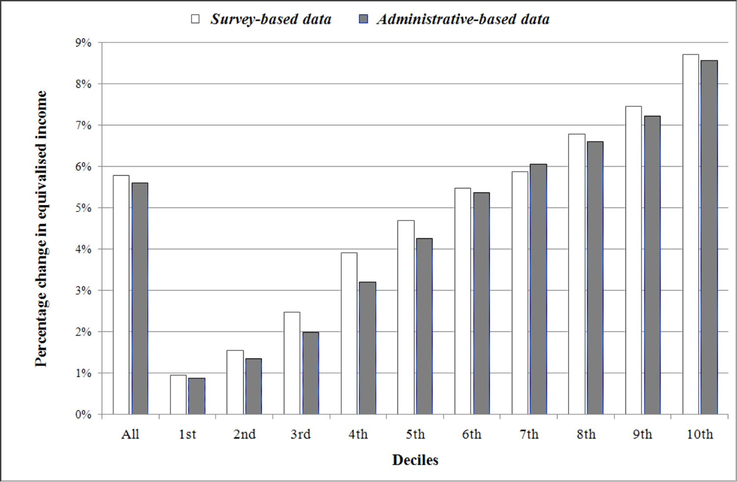
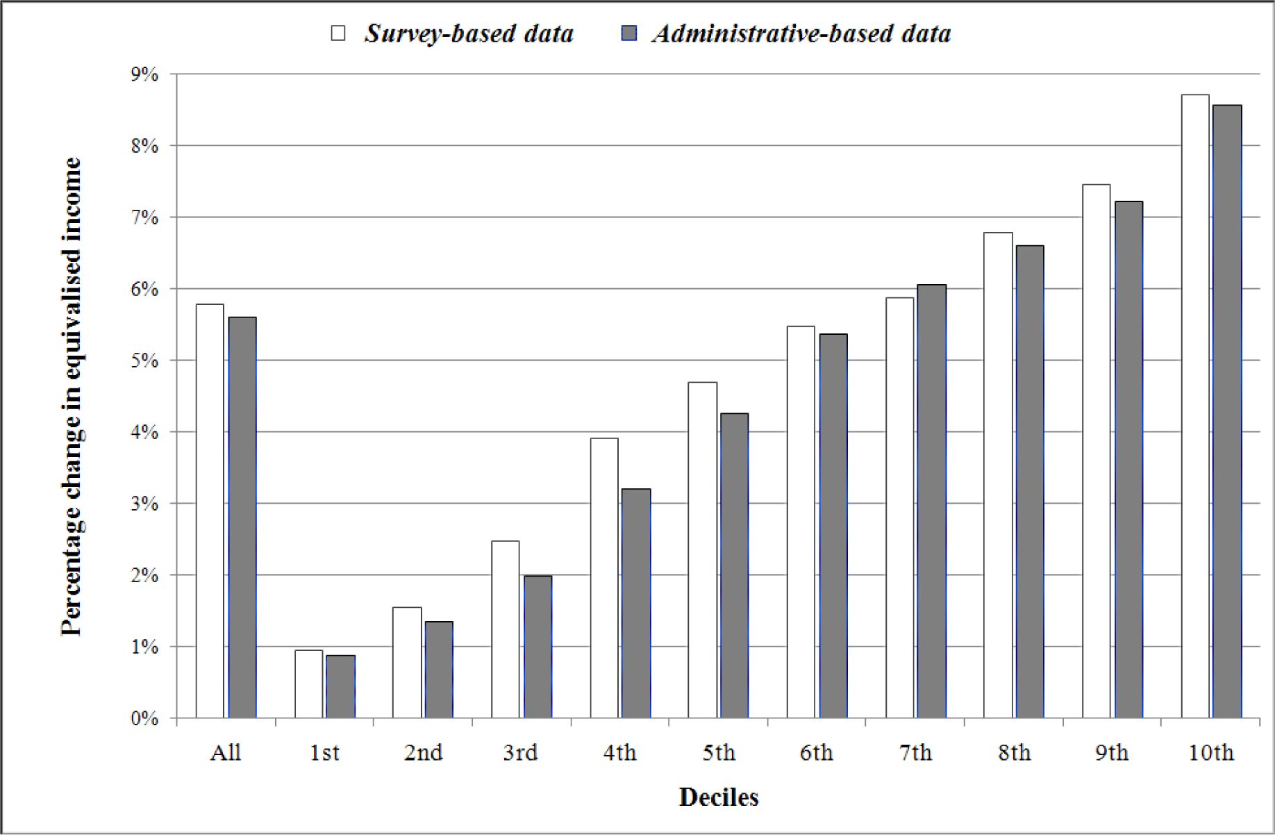
Relative change in mean equivalised income due to the tax reform, by decile (*)
Source: PSELL3/EU-SILC, 2004, Luxembourg Social Security Data Warehouse, 2003, and EUROMOD computations
(*) Deciles of equivalised income distributions are determined with and without tax reform, separately, and then compared.
First we explore the impact of taxation. Estimates of the before-tax Gini index based on survey and administrative data are very similar (0.297 and 0299 respectively). Estimates of the post-tax Gini index are also highly similar, regardless of the tax system in force. In all cases it decreases, varying significantly more between fiscal systems (0.23 without tax reform; 0.25 with tax reform) than between datasets (where the measurable difference is of the order of only 0.002-0.003). This drop in the inequality coefficient is mainly due to vertical redistribution19 of the tax system (Reynolds-Smolensky index). The horizontal redistribution20 appears to be negligible. Here again, results stemming from the two datasets are similar.
Next we examine post-tax differences in outcome for the fiscal system alternatives under consideration. Table 6 clearly shows that the values of the inequality coefficients are increased due to the 2001–2 tax reform, meaning that the inequalities in the distribution of equivalised income are amplified. This is illustrated by Figure 1, which shows the change in mean equivalised income by decile. On the whole, the 2001–2 tax reform increases equivalised income, with the size of the increase dwarfing the difference between datasets (5.6% according to our survey-based data; 5.8% according to our administrative-based data). Moreover, the higher the decile, the higher the relative change. A 9%-increase of mean equivalised income is observed when considering the highest decile compared with less than 1% for the lowest decile, whatever the dataset. Again, regardless of decile, the difference in estimated increase between datasets is far smaller than the size of the estimated size of that increase.
The reinforced income inequality is largely explained through a reduction of the Reynolds-Smolensky index of vertical redistribution. This can be further decomposed into ‘progressivity’ (Kakwani index) and ‘magnitude’ (a coefficient depending on the average rate of taxation), both factors playing a positive role in the vertical redistribution. Yet again differences in these indicators attributable to changes in fiscal systems are far larger than those due to data source (survey or administrative data).
Regardless of data source, the decomposition helps in understanding what is at stake in the tax reform. Clearly, the reduction in vertical equity due to the reform results from a drop in the rate of taxation of 5.0-5.1% and not from the progressivity, which increases from 0.342/0.357 to 0.411/0.430 as measured by the Kakwani index21.
In summary, what is most striking in Figure 1 and Table 6 is the consistency between effects whether changes are measured using administrative-based or survey-based data. In fact only one element, found in Table 6, shows a greater difference between datasets than between fiscal systems. This difference, already discussed in Section 3.4, is the Atkinson index calculated with an inequality version of 2.
4. Conclusions
In this paper we have initiated, through the EUROMOD microsimulation framework, the cross-validation of administrative data derived from the recently implemented Luxembourg Social Security Data Warehouse, on the one hand, and of the PSELL3/EU-SILC survey data, on the other hand. This case study is, we believe, of wider interest because of the lessons it has to offer regarding the relative strengths and weaknesses of survey and administrative datasets as inputs for microsimulation models. In particular, the nature of any discrepancies and the importance of these discrepancies relative to the kinds of differences likely to be observed downstream when modelling changes in fiscal systems are examined in the paper. Given the lack of previously peer-reviewed work in this area, we also hope that this paper might offer some valuable pointers to others considering embarking on a similar cross-validation exercise. We summarise our approach and main findings below, before moving on to consider possible future refinements.
Before comparing our survey and administrative datasets we endeavoured to eliminate as many dissimilarities as we could control for, including the target population, the lack of precision in some important (income-related) variables and the time-frame covered (we have restricted ourselves to 2003). As a result of this process of harmonisation we had to drop about 6% of the initial population in both datasets and adapt the calculation of variables such as those related to capital income-related due to missing information in the administrative dataset. For the same reason it also proved necessary to adopt the fiscal household as the unit of analysis rather than the more usual resident household. Because fiscal households nest within residential households, this led to an observed distribution of equivalised income that departed from the usually observed residential-based ones, with lower values for both means (5% less when fiscal households are used) and medians (-6%). The at-risk-of-poverty rate and the position of the different categories of population were also affected.
Following harmonisation the two datasets appear to be satisfactorily similar with regards to several non-monetary characteristics, such as age classes and types of household. For monetary characteristics, a discordance is observed, mainly stemming from a gap in primary income, which is, on average, 7% lower in administrative-based data. The difference in primary income implies downstream effects on equivalised income. Even so, while the average equivalised income differs, the shapes of the income distributions recorded in the two datasets broadly coincide. For example, the Gini coefficient and other overall inequality indices most often show a statistically compatible distribution of equivalised income in the two datasets. The same most at-risk-of-poverty categories also show up regardless of the dataset under consideration, including ’singles with dependent(s)’ and the members of (fiscal) households in which either nobody or only one person is working.
The exception is the occurrence of some notable discrepancies at the extremes of the income distribution. For example, at the lower end of the income distribution, the survey-based data provide higher estimates of the at-risk-of-poverty rates for most of the population sub-categories considered. Moreover, inequality indices focusing on the poorest households, like the Atkinson index with a high aversion to inequality, show some divergence between the two datasets. In this latter case it can be shown that differences in the first percentile of the distributions are sufficient to explain the divergence. At the other extreme of the distributions, a few striking differences were also noticeable between the datasets. These deviations are explicable in terms of known distortions in the collection of data regarding higher income levels.
Having compared the ‘level’ and ‘distribution’ of income captured via survey and administrative data, we concluded by considering the impact of the discrepancies observed on a microsimulation analysis of three alternative fiscal scenarios. By deliberately applying all three fiscal systems to the observed 2003 population, we have avoided the problem of observing changes that are not directly the result of changes in the tax system itself. Our results show that, with the exception of one measure (Atkinson index with inequality aversion = 2), the discrepancy between datasets in the estimated values of a wide range of inequality indicators was far smaller than the observed change in inequality indicators between fiscal systems.
On the whole, therefore, we can conclude from comparisons of both ‘levels’ and ‘policy impacts’ that our survey database performs reasonably well in capturing the relevant characteristics of population shared in common with our administrative dataset. Even if some variables may differ, on average, the shapes of the equivalised income distributions are similar, and the changes due to policy alternatives are most often remarkably comparable. Making the assumption that the survey data are equally representative of the elements of the resident population over-looked for the purposes of cross-validation, our survey dataset appears to offer the scope to undertake analyses with respect to characteristics not found in our administrative database (and vice versa).
Of course, our conclusion is based upon cross-validation of outcomes arising from the treatment we have chosen to impose to the initial datasets to make them target closer populations and to get rid of the effect of some income-related missing or unevenly biased variables. A next step is to explore alternative avenues for validating those elements of our datasets not covered directly by this cross-validation, with a view to reducing the number of data interventions required. An important extension concerning administrative data in Luxembourg would also be to properly deal with (postal) addresses, after improvement in their normalization. The objective would be, for example, to make resident and institutional households identifiable and spatial analysis feasible. We could also profit, in the future, from available complementarities between
administrative and survey data and create an operational link, for example, through statistical matching or actual matching (subject to the limitations imposed by the statutory protection of data privacy). This would also help in introducing into our administrative data a variable crucial for most socio-economic analyses: education.
Footnotes
1
Panel Socio-Economique Liewen zu Lёtzebuerg; (http://www.ceps.lu).
2
EU-SILC is an instrument aiming at collecting timely and comparable cross-sectional and longitudinal multidimensional microdata on income, poverty, social exclusion and living conditions (see http://epp.eurostat.ec.europa.eu/portal/page/portal/microdata/eu silc).
3
4
Minimum Social Wage = €1368.74 per month as of 1 January 2003.
5
Either married all through the year or married during the (civil) year, or divorced during the year.
6
If unmarried parents, the child goes to his mother’s household, unless there is an explicit demand from the mother to link the child with his father concerning the family benefits. If born during the year or when family benefits come to an end during the (civil) year, a child is still linked to the household of his parent(s).
7
Information for non-residents is partially available in the Data Warehouse.
8
Source: STATEC – National statistical institute of Luxembourg (http://www.statistiques.public.lu).
9
For a detailed presentation of social indicators, see Atkinson et al. (2002) and Marlier et al. (2007).
10
Total disposable income = (earnings – social contributions – taxes + social benefits) summed up for all members of the household.
11
The Gini coefficient takes a value between 0 (minimum inequality) and 1. If we define the social welfare as , then it can be shown that W(x) = μ * ( 1 – G), where n is the number of individuals, xi/j is the income level, μ is the average income, and G is the Gini inequality index. See Essama-Nssah (2000) and Lambert (1993).
12
The Atkinson inequality index can be expressed as , where n is the number of individuals, xi is the income level, μ is the average income, and is the inequality aversion coefficient. It takes a value between 0 (minimum inequality) and 1 and can be interpreted in terms of social welfare; it shows that part of total income which might be saved, while keeping the social welfare (associated to the Atkinson index) unchanged and distributing the remaining disposable income equally. The higher the value of ε, the stronger the impact of the left side of the distribution on the index. See Essama-Nssah (2000) and Lambert (1993).
13
This would be statistically compatible if a 99% confidence interval.
14
A decomposition of inequality indices by population sub-group could also enlighten the question.
15
As this difference falls outside the 95% confidence interval for the survey-based poverty rate (10.5% – 12.5%), it also appears to be statistically significant.
16
However, the difference is not statistically significant at the 1% level for the former category.
17
The Foster-Greer-Thorbecke poverty index with parameter 1, which is the product of the poverty rate and the income gap ratio, is shown to be 0.015 through survey-based data (respectively 0.016 through administrative- based data), leading to an income gap ratio of 0.015/0.115 = 13% (resp. 17%). The income gap ratio = 1 – (Mean income of the “poor”/Poverty line); it refers to the extent to which the incomes of the poor lie below the poverty line.
18
If the first percentile of the equivalised income distribution is left out, the Atkinson index with an inequality aversion of 2 drops from 0.226 to 0.159 for administrative-based data. It is much more slightly modified for survey-based data, from 0.168 down to 0.156 with a 95% confidence interval, which becomes [0.1490.162]. For a more general analysis of such tendencies, see Van Kerm (2007).
19
Vertical redistribution consists of reducing inequalities of equivalised income between households who have the same structure but a different income level.
20
Horizontal redistribution consists of reducing inequalities of equivalised income between households who have the same income level but a different structure.
21
The increase in progressivity can be explained by an enlargement of the first tax bracket (tax rate = 0%), which overcomes, regarding the measurement of progressivity through the Kakwani index, the effect of reducing the marginal tax rates for higher income levels.
The tax system in luxembourg and the 2001–2002 tax reform
In Luxembourg, the tax unit is the ‘family’, which might not include all members of a ‘resident/nuclear household’. To belong to the same family, one must either be (official) spouse or a dependent child. Two cohabiting persons who are not married are then members of separate tax units. A ‘child’ belongs to his/her parents’ tax unit if unmarried and less than 21 years old. As soon as he or she is married, a son/daughter enters his/her own tax unit. The same prevails if a person is older than 21 years and is neither a student nor a disabled person. Of course, the set of rules includes many other aspects related to the questions of ‘earnings’ of dependent children, children living part-time only with their parents, status changing during the civil year, spouses separating/being divorced, etc. These questions, although essential to the system as a whole, are not discussed here.
The main outlines of the 2001–2002 reform in Luxembourg are described below:
The first tax bracket is enlarged, which means that the minimum income before tax is increased, from 6,693 EUR in 2000 to 9,750 EUR in 2002.
The number of tax brackets is reduced from 18 to 17 in 2002 and bandwidths are made uniform to 1,650 EUR in 2002.
The maximum tax rate significantly decreases, from 46% to 38% in 2002
The year 2003 is chosen as a basis for analysis. In the benchmark, the tax system is designed as in 2003, which is just after the implementation of the 2001–2002 tax reform, conforming to the brief description made earlier. The alternative is then simply to set up the tax system as of 2000, which means in its pre-reform state. On the benefit side, no change is made between the benchmark and the alternative.
References
- 1
-
2
Micro-simulation in action: policy analysis in Europe using EUROMODAmsterdam: Elsevier.
-
3
Les effets redistributifs de la politique familiale, Etude réalisée pour le compte du Ministère de la Famille du Grand-Duchéde Luxembourg: CEPS/INSTEAD.
-
4
Assessing the Impact of Tax/Transfer Policy Changes on poverty : Methodological Issues and Some European EvidenceUnited Kingdom: University of Essex.
- 5
-
6
Using the EU-SILC for policy simulation: Prospects, some limitations and suggestions. EUROMOD Working paper, EM1/07United Kingdom: University of Essex.
-
7
Effect of changes in tax/benefit policies in Austria 1998–2005. EUROMOD Working paper, EM3/07United Kingdom: University of Essex.
-
8
The Impact of Inflation on Income Tax and Social Insurance Contributions in Europe. EUROMOD Working paper, EM2/00United Kingdom: University of Essex.
-
9
The distribution and redistribution of income (2nd Ed)Manchester: Manchester University Press.
-
10
Cross-validating administrative and survey datasets through microsimulation and the assessment of a tax reform in LuxembourgUnited Kingdom: University of Essex.
- 11
-
12
An analysis of the effects of using interview versus register data in income distribution analysis based on the Finnish ECHP-surveys in 1996 and 2000. CHINTEX Working Paper #15Finland: Abo Akademi university.
-
13
Interview and register data in income distribution analysis. Experiences from the Finnish European Community Household Panel in 1996Helsinki: Statistics Finland.
-
14
Modelling Our Future: population ageing, health and aged care. International Symposium in Economic Theory and Econometrics483–488, EUROMOD: the tax-benefit microsimulation model for the European Union, (eds), Modelling Our Future: population ageing, health and aged care. International Symposium in Economic Theory and Econometrics, Elsevier, 16.
-
15
Extreme incomes and the estimation of poverty and inequality indicators from EU-SILC. IRISS Working paper, 2007–01Luxembourg: CEPS/INSTEAD.
Article and author information
Author details
Acknowledgements
The research presented in this paper is part of the REDIS project (Coherence of Social Transfer Policies in Luxembourg through the use of microsimulation models) funded by the Luxembourg National Research Fund under Grant FNR/06/28/19. We are grateful to Isabelle Debourges (IGSS) for her helpful assistance with the data and two anonymous referees, together with the editor of the International Journal of Microsimulation, for many stimulating suggestions. The paper was first presented at the Conference on Tax-benefit Microsimulation in the Enlarged Europe: Results from the I-CUE Project and Perspectives for the Future, Vienna, 3–4 April 2008. We are grateful to participants for helpful comments. Of course, we are solely responsible for any remaining errors.
Publication history
- Version of Record published: April 30, 2011 (version 1)
Copyright
© 2011, Liégeois et al.
This article is distributed under the terms of the Creative Commons Attribution License, which permits unrestricted use and redistribution provided that the original author and source are credited.