Micro simulations on the effects of ageing-related policy measures: The social affairs department of the Netherlands Ageing and Pensions Model
- VU University Amsterdam, Amsterdam
- Ministry of Social Affairs and Employment, Den Haag
- Article
- Figures and data
-
Jump to
- Abstract
- 1. Introduction
- 2. Background
- 3. Modelling redistribution within the state pension system
- 4. Modelling the retirement decision of employees
- 5. Model results
- 6. Conclusions and topics for future research
- Footnotes
- The SADNAP Model
- Data sources
- Baseline results
- References
- Article and author information
Abstract
This paper describes a newly extended version of the dynamic micro simulation model SADNAP (Social Affairs Department of the Netherlands Ageing and Pensions model). SADNAP is being developed for calculating the financial and economic implications of the ageing of the population and of the ageing-related policy measures that are being proposed to cope with ageing. The model uses administrative datasets of Dutch public pension payments and entitlements for both public and private pensions. SADNAP has already been in use since 2007 for forecasting the state pension expenditures and for analysing the budgetary effects of policy changes.
The model has been extended in order to give a broader assessment of policy alternatives by providing insight into other important evaluation indicators like income redistribution and the retirement decision of workers. For the modelling of income redistribution a new micro data source with individual data on private pensions is combined with differentiation of mortality rates in order to gain a better insight in the income at the individual level within the population of pensioners. For the modelling of the retirement decision an option value model is developed in which key parameters vary at the individual level in order to benefit from the micro simulation approach. These extensions greatly enhance the performance of SADNAP. Besides the financial implications, additional insight can now be provided into the effects of policy measures on a set of key indicators.
In this paper both extensions are described in detail and a complete baseline projection of all key indicators is discussed.
1. Introduction
The Netherlands, like most OECD-countries, is facing an ageing population. Especially, this is a complication for the state pension, known as AOW (Algemene Ouderdoms Wet), which is financed through a pay-as-you-go system. The state pension is the first pillar in the Dutch pension scheme, which is based on three pillars. The second pillar consists of supplementary company or occupational pension facilities. Employees are obliged to take part in those second-pillar pension programmes. The third pillar contains individual pension saving programmes in which participation is voluntarily. Both second and third-pillar pensions are fully funded.
The dynamic micro simulation model SADNAP (Social Affairs Department of the Netherlands Ageing and Pensions model) is being developed for calculating the financial and economic implications of the ageing problem and of the policy measures considered. A micro simulation model, as compared to macro-oriented models, can give more detailed information on the ageing problem and on the redistributive effects of policy options, which can be used in the evaluation of those options. The model uses administrative datasets of all Dutch public pensions and entitlements for all public pensions and a large share of private pensions.
The structure of this paper is as follows. Section 2 gives a brief overview of the Dutch pension system, the forecasting models currently in use at the Ministry of Social Affairs and Employment and a short general introduction to micro simulation models and the SADNAP model. Sections 3 and 4 present in more detail two recent extensions of the SADNAP model. Section 3 focuses on the modelling of incomes and redistribution within the state pension system and in Section 4 the modelling of the retirement decision using the option value approach is described. In Section 5 the main results of the model are presented. These results are limited to the baseline scenario of unchanged policies. A separate paper is dedicated to an evaluation of different policy options with the model. Section 6, finally, contains conclusions and some topics for future research.
2. Background
2.1 The dutch pension system
The Dutch government supplies a state pension called AOW to all persons aged 65 or over when they become entitled. Inhabitants of the Netherlands build up a right to this pension by living in the Netherlands while aged between 15 and 65. The state pension accrues at the rate of 2% for every year this condition is fulfilled. Part of the population is only partially entitled because they have not lived in the Netherlands continuously between the ages of 15 and 65. This share of incomplete state pensions is rising because of the growing number of immigrants during the last few decades.
The state pension scheme provides a basic minimum income guarantee in case of a full entitlement. Therefore the system makes a distinction between partners of a couple and single persons. A single person is entitled to 70% of the net minimum wage1 and a member of a couple is entitled to 50% of the net minimum wage. Until 2015, persons with a (non-working) partner younger than 65 can supplement their state pension of 50% with an allowance of another 50% to a combined maximum of 100% of the minimum wage. Partially entitled persons can claim social assistance. Social assistance, however, is income and means tested.
The AOW is a pay-as-you-go arrangement, the current population of workers pay for the current population of pensioners. Hence the AOW is financed through a premium paid by these workers. The premium is fixed at a rate of 17.9% of the first two tax brackets (the limiting income is approximately € 32,000 in 2009). Revenue from this premium is not sufficient to cover all AOW costs, however. The government contributes the part of the AOW costs (currently about one third) that is not covered by the premiums. The government contribution is financed by taxes, which are paid by pensioners as well.
The importance of second and third-pillar pensions for the income position of the elderly is growing as more people are saving for such pensions and their average savings are increasing. Per person average second-pillar pension savings are almost equal now to the average first pillar state pension savings. In the future, it is to be expected that second and third-pillar pensions together will provide more than half of the average pension income. Although there are many second-pillar pension funds in the Netherlands, each with its own rules on contributions and pensions, broadly speaking one can say that pension funds try to supplement the state pension to a total gross income level of 70% of the pensioner’s final wage. Most pension funds have recently switched from a final wage system to a career average system, but on average they still aim for a gross pension level of 70% of the final wage. Because pensioners no longer have to pay state pension contributions, the net height of their first and second-pillar pensions together usually, in the case of a full pension, comes close to 90% of the final wage. Other income sources, like third-pillar pensions can add to this income level.
2.2 Models currently in use
The Ministry of Social Affairs and Employment is responsible for preparing state pension forecasts for the yearly budget. The budget horizon is six years (the current budget for 2010 contains forecasts from 2009 until 2014). Although beyond the budget horizon, the long-term forecast of pension expenses is of great importance as well because government budgets are also affected by the long-term sustainability of public finance. Besides the financial effects for the government budget, the Minister of Social Affairs and Employment is also responsible for income policies and labour participation policies. When new policy options are discussed, a broad analysis of both short-term and long-term financial effects, income effects and labour participation effects will be required. Moreover, in the case of ageing-related policy measures, income effects will not be limited to direct effects on purchasing power but will include intra-generational and inter-generational redistribution issues as well. In order to assess all these effects, a number of different models are used.
For state pension expenses, a simple macro model is used, using forecasts of the number of pensioners for the most relevant subgroups of the state pension population (men and women, singles and couples with and without a partner allowance, complete and reduced pensions). These volume forecasts are supplied by the state pension administration office (SVB). The macro model calculates the costs by multiplying the expected group sizes with the average pensions for each group. As the SVB forecasts project ahead as far as 2024 and rely heavily on extrapolating existing trends, for the long-term development of the state pension expenses, the Ministry relies on a macro AGE model of CPB. This model, called GAMMA (see Van Ewijk et al., 2006), is used once every four years (in the run-up to the general elections) for a long-term forecast of the whole Dutch economy. For income effects, the long running static micro simulation model Micros (Hendrix, 1993) has been used since the early 1990s. This model focuses on the short-term income effects of complex sets of policy measures. Labour participation effects are quantified on an ad-hoc basis using recent research papers by CPB and others. Redistribution effects are mostly abstracted from or quantified on an ad-hoc basis as well.
This approach has several shortcomings. Because different models from different internal and external sources are used, it is very difficult to obtain a consistent picture of the effects of policy measures. Besides, the Ministry is highly dependent on other institutions for supplying information and forecasts. Therefore, it can be difficult to anticipate and respond quickly to policy developments. Also, the quality and richness in detail of the forecasts can be improved by using one consistent micro simulation model.
In the first place, information does get lost because the macro model uses only a small number of groups sharing the same basic characteristics. Age groups are not included, for example, although among the population of persons aged 65 and over, different ages may have very different characteristics. Second, there are certain features of the AOW that cannot simply be taken into account with macro models, such as changes in migration patterns and changes in household situation. Migration affects the entitlements to the AOW because the AOW- entitlement depends on citizenship. Changes in the number and age of immigrants and emigrants will affect the pension expenses later on. The AOW-entitlement also depends on household situation. Two single persons receive a higher pension than two persons in a couple, so when the number of singles among the population of pensioners rises, the cost of the AOW will rise as well. Third, the macro models are limited to the state pensions, that provide the basic income level, whereas the main differences in the income positions of pensioners are caused by private pensions. The Micros model, which is used for the income effects, is a static model that is not capable of adequate long-term forecasts. Fourth, the effects on labour participation and income redistribution are not captured at all by the current models in use at the Ministry.
Therefore the Ministry has been developing the dynamic micro simulation model SADNAP to handle the problems just mentioned. SADNAP is an integral ageing and pensions model, including the income and redistributive effects of different policy measures. The purpose of SADNAP is to provide consistent and integral forecasts of both short-term and long-term effects of the baseline scenario of unchanged policies and various policy measures on the cost of state pensions for government budget, the income position of the elderly, redistribution and labour participation. SADNAP has already been used for budgetary forecasts since 2007.
2.2. Micro simulation models
Micro simulation basically is a modelling technique that uses large datasets containing data on the individual level. Records on individual persons contain characteristics like birth year, gender, ethnicity, income level, household status etc. Transition probabilities and institutional rules are applied to simulate whether events will happen in the future to a specific record, e.g. whether someone starts working or finishes a relationship. Calculation rules are used to apply the probabilities and institutional rules to the micro data file. The result is an estimate of the outcomes of applying these rules, including both the total aggregate change and the distributional nature of that change.
Micro simulation models can be subdivided in many different ways (O’Donoghue, 2001). The most important one is between dynamic and static models. With dynamic micro simulation the characteristics of a record can change over time. Static micro simulation does not allow characteristics to change. Although in static simulations reweighing techniques can be used to allow for changes in population composition, static micro simulation is usually seen as more suited for short-term forecasts, like the short-term impact of fiscal measures, whereas dynamic micro simulation is seen as more suited for long-term forecasts like the impact of ageing.
Micro simulation is subject to Monte Carlo variability, resulting in different outcomes for each individual simulation experiment. Of course, a larger sample can reduce the fluctuations between different runs with the model, but not eliminate them. Moreover, in large dynamic micro simulations sample size can still be limited due to disk capacity or computer speed. One can deal with the Monte Carlo variability in several ways. First, several simulations can be done and an average outcome can be calculated. The difference in average outcome between the base situation and the policy alternative can then be accounted to the policy change. A second approach is proposed by Klevmarken (2007), who describes a calibration technique in which the simulation results are aligned to an a priori defined target, such as a macro forecast, eliminating the variability. Third, Monte Carlo variance can be avoided completely by using a fixed set of random numbers used to generate the events. This last method is useful to allow for replication of model results and to compare policy alternatives to the base situation, because when the random numbers are fixed, differences between two simulations can only be caused by the policy change. For every individual a simulation of a policy alternative can then be performed under exactly the same conditions as the simulation of the baseline scenario. In SADNAP, both calibration and fixing of random numbers are used.
Micro simulation is very useful when information for specific individuals or groups of individuals is needed. Information on specific groups can also be obtained by creating more groups within cell-based macro forecasts. In practice, however, because of the large number of subgroups that arise when taking into account all the relevant characteristics, these cell-based approaches become problematic when the subgroup size becomes too small (Van Sonsbeek & Gradus, 2006).
However, construction of a dynamic micro simulation model can be very complex and time consuming. This holds true especially for a dynamic population model, which requires replacing the starting population with new cohorts over time. Cassels, Harding and Kelly (2006) identify some success and failure factors and recommend that models should have clear objectives, a modular design, be user friendly, produce timely output and be transparent. With SADNAP these recommendations have been followed by initially limiting the model to the budgetary impact of the state pensions only.
2.4. The sadnap model
The Ministry of Social Affairs and Employment has been developing the SADNAP model since 2006. As the model is modularly designed, attention was first focused on the demographic model and the state pension forecast. Therefore, since 2007 the SADNAP output has been used in preparing the state pension budget forecasts of the Ministry. An early project description is documented in Van der Werf, Van Sonsbeek and Gradus (2007). In later years, the original demographic modules have been extended. The immigration and emigration code has been improved in order to allow for the interdependency between the two (immigrants having a higher emigration rate). Also, the take-up of state pensions by former emigrants has been incorporated in the model. The household formation code has been improved in order to provide reliable relationship patterns at the micro level. In a new module, non-budgetary aspects (like income distribution and labour participation/retirement decision) have been introduced in order to gain a more complete picture of the pros and cons of different ageing-related policy measures.
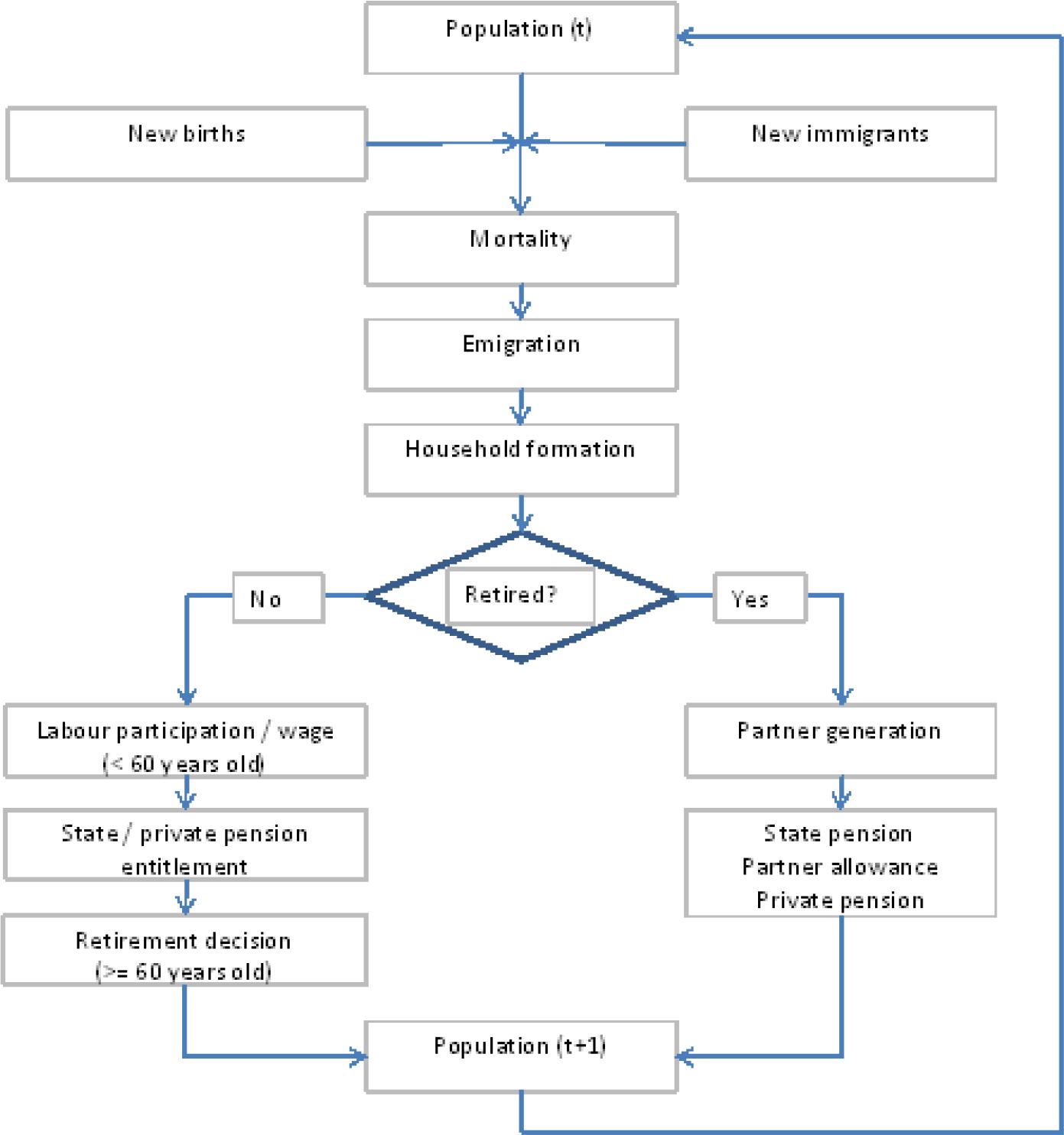
In the early versions, the income was limited to the state pension (building up of entitlements for the population aged 64 and below and pension payments for the population aged 65 and over). The income position has now been supplemented with private pension data, first with rough estimates based on aggregate data and subsequently with a full micro data set on private pension entitlements which has been supplied by Statistics Netherlands. A detailed description of the demographic and income modules of SADNAP is given in appendix A and a detailed description of the micro and macro data sources used in SADNAP is supplied in appendix B. The flow diagram of the SADNAP model is given in Figure 1.

SADNAP model flow diagram.
This paper focuses on two extensions of the SADNAP model which have been implemented recently. The first is the differentiation of mortality rates that is used to investigate the redistribution within the state pension scheme, and which is described in Section 3. The second is the modelling of labour participation and the retirement decision, which is described in Section 4. Both extensions fill the gaps that were left in the assessment of policy alternatives as described in Section 2.2.
2.5. Comparison with other dynamic population micro simulation models
Within the Netherlands, SADNAP is the second attempt to develop a dynamic population micro simulation model capturing ageing issues. The only comparable model in the Netherlands is the NEDYMAS model (Nelissen, 1993), which was prominent during the 1990s. Although SADNAP, as compared to some well-known international simulation models, is a comparatively simple and small-scale project, it shares some key characteristics with these larger models. Cassels, Harding and Kelly (2006) present an overview of six large dynamic population micro simulation models (Dynasim3 from the USA, Dynacan from Canada, Mosart from Norway, Sesim from Sweden, Sage from the UK and Dynamod from Australia). Like all the models but Dynamod, SADNAP is a discrete model with one year time steps. The development platform is SAS, as in Dynasim3. The sample size (1-2%) is comparable to most models (e.g. Dynacan, Mosart, Dynamod). The time horizon (2080) is also comparable to for example, Dynacan and Mosart (2100). In SADNAP results are aligned to targets taken from macro data sources. As in, Dynacan, for example, alignment targets include rates for mortality, fertility, migration, marriage and divorce propensities. As in most of the models mentioned, SADNAP contains modules on population, household formation, labour force participation, benefits and taxation.
However, there are some simplifications as compared to the larger models. For example, household formation in SADNAP is a binary choice between single and cohabiting, which excludes, for example, children leaving home, people moving in and out institutions and adults living in other households without family relations (cf. Mosart). Taxation is included in SADNAP as in most other models (except Dynacan) but is simplified to the main tariff structure. Education and health are abstracted from SADNAP. Financial wealth and savings are also abstracted, but they are planned for an extension in the future. SADNAP is comparatively narrow in scope, like for example Dynacan, so most effort is put into subjects directly related to pensions and ageing. In the current SADNAP version, most effort has been put into the retirement decision model, which consequently is comparatively elaborate.
3. Modelling redistribution within the state pension system
The Dutch state pension scheme can be classified as a “Beveridge”-style public pension programme (Disney, 2004), characterized by significant departures from actuarial fairness and significant provision of private retirement benefits, as opposed to “Bismarck”-style public pension programmes, characterized by high actuarial fairness and limited private provision of private retirement benefits. The Dutch scheme, with its flat-rate pensions for single persons and cohabitants, therefore has a highly intragenerational redistributive character.
There is also redistribution from higher to lower incomes because higher income earners contribute more to the scheme during their lifetime. However, this only holds true for income differences up to the limiting income of approximately € 32,000 (in 2009). For the moment, this kind of intergenerational redistribution is not included. Additional research has to be done in order to identify which groups have a better balance of withdrawals as compared to their contributions.
Typically, subgroups with lower life expectancies on average contribute more than they withdraw from the scheme. Well known factors affecting life expectancy are gender, income, marital status and ethnic background. Gender- and age-specific mortality rates are derived from the CBS population forecast and were used in SADNAP from the beginning. However, there are also notable differences in mortality rates between different income levels, between single persons and couples and between different ethnicities. From a redistribution perspective those differences are important although they are not easy to implement in a simulation model because of alignment problems. Moreover, these possible causes correlate, complicating the analysis of the ground cause of the differences in mortality.
On the relationship between income and life expectancy, in a large Finnish study Martikainen et al. (2001) show the mortality rates of the lowest income decile on average to be 2.37 times as high for men over 30 years of age and 1.73 times as high for women over 30 years of age as those in the highest income decile. On the relationship between marital status and life expectancy, de Jong (2002) shows the mortality rates of married people to be significantly lower than those of single, divorced or widowed persons. The difference is larger for men than for women, and increases in time for both men and women. However, the differences in mortality rates are smaller in the higher age categories. On the relationship between ethnic background and life expectancy, Bos et al. (2004) show mortality to be higher among three of the four largest groups of immigrant males in the Netherlands. However, among Moroccan males, mortality appeared to be lower and among females in general, inequalities in mortality were small. Moreover, mortality rates were influenced by marital status and socioeconomic status, leaving a smaller influence of ethnic background in itself, except for younger age categories. This contrasts with data from SVB (2008) showing the mortality age of people not born in the Netherlands, to be significantly lower than that of people born in the Netherlands, with differences in average mortality age of more than 10 years between natives and Turks and Moroccans. On average, people with reduced state pensions, including most first generation immigrants, live four years less than people with full state pensions, according to this study.
In SADNAP, the differences in mortality rates by income are derived from the study of Martikainen et al. (2001). The expected total private pension is used as a proxy for income. This means that people do not move between income deciles, only one “lifetime” decile is assigned per person. The estimation of the pension entitlements has been improved recently because a detailed micro dataset of company pensions has become available. This dataset is described in appendix B. The wage level of the participants is known for the base year. Their pension entitlements are based on continuation of their current wage level throughout their working life. That means that, the younger one is in the base year, the less accurate the pension entitlement forecast is as wages are expected to rise during the working life. Wages in the Netherlands are strongly correlated with age. Figure 2 presents the average wages and expected pensions by age based on the 2005 micro dataset. The picture strongly resembles earlier findings on age-earnings profiles like those from a longitudinal Dutch survey (Alessie, Lusardi & Aldershof (1997) and more recently Kalmijn & Alessie (2008)). They found that the age-earnings profile shows a steep profile for the young, subsequently a moderate increase over the life cycle and finally a sharp decline well before the mandatory retirement age of 65.
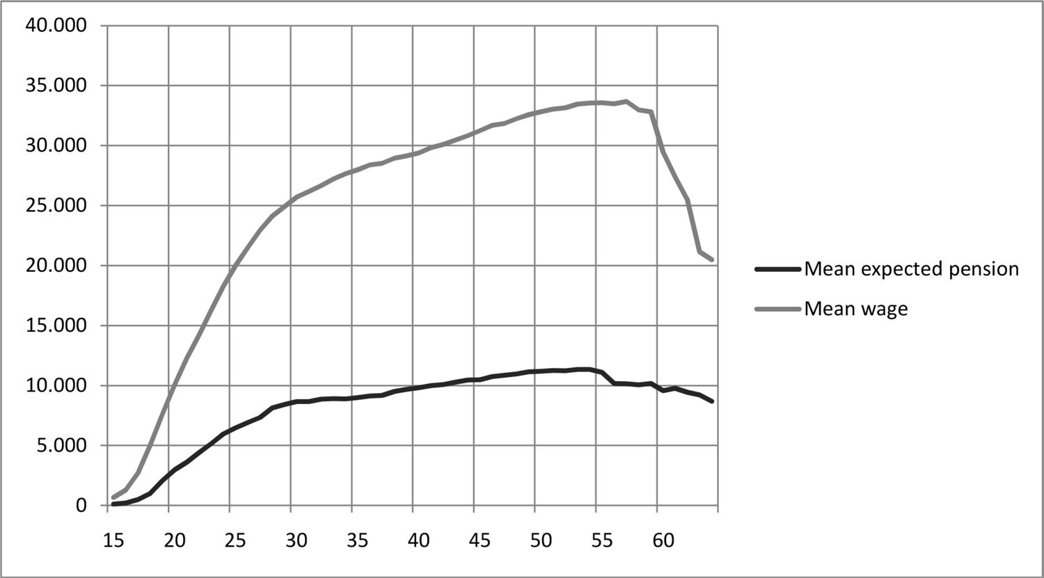
Average wage and expected second-pillar pension by age.
Currently SADNAP lacks the more elaborate modelling of wages over the life cycle of, for example, Borella and Coda Moscarola (2005). However, when wages and pension savings are assumed to follow each other’s development over the life cycle, the replacement rates will remain the same. Only, as earlier noted, the replacement rates for the youngest age cohorts provide no good guidance for the replacement rates at older ages. Figure 2 suggests that from age 30–35 onwards reasonably accurate projections of future income development can be made.
By introducing this difference in mortality rates by income, differences in mortality rates by household status and ethnic group are introduced at the same time, as single persons on average have lower incomes than cohabitants and immigrants on average have lower incomes than natives. This also results in higher mortality among people with reduced state pensions, mainly immigrants, an observation that also is made in SVB (2008). A further difference in mortality rates between single persons and cohabitants and between natives and immigrants is introduced in order to increase the differences in life expectancy to the levels reported in the studies of de Jong and Bos et al. respectively.
Table 1 shows the life expectancies (at age 65) for different subgroups of the population of pensioners for the 2006–2045 cohorts of pensioners (the 1941–1980 birth cohorts). As the simulation runs until 2080, the 2045 pensioner cohort is one of the last cohorts that will have almost completely died out by 2080. Besides the familiar difference in life expectancy between men and women, there are also sizeable differences between different income groups, between cohabitants and single persons and between natives and non-natives. The differences between income groups are in line with recent Dutch research byKalwij, Alessie and Knoef (2009). The average expected age of the cohorts turning 65 is 86. This is consistent with CBS (2009) in which life expectancy at 65 years old rises from 19.4 years (17.8 for men and 21.0 for women) in 2009 to 21.8 years (20.8 for men and 22.9 for women) in 2045. The difference in life expectancy between men and women is decreasing over time until a difference of about two years is left. The differences in life expectancy between income quintiles, single persons and cohabitants and natives and first generation immigrants are assumed to remain constant over time.
Average life expectancies at 65 of the 2006–2045 pensioner cohorts.
| Subgroup | Average mortality age | Δ Average |
|---|---|---|
| By income | ||
| - 1st quintile | 83.5 | -2.5 |
| - 2nd quintile | 84.5 | -1.5 |
| - 3rd quintile | 85.6 | −0.4 |
| - 4th quintile | 86.8 | +0.8 |
| - 5th quintile | 88.5 | +2.5 |
| By gender | ||
| - Women | 86.9 | +0.9 |
| - Men | 85.1 | −0.9 |
| By household status | ||
| - Singles | 84.4 | −1.6 |
| - Cohabitants | 86.7 | +0.7 |
| By origin | ||
| - Natives | 86.6 | +0.6 |
| - Immigrants | 84.0 | −2.0 |
| Total | 86.0 |
The population decomposition used allows for an analysis of redistribution within the state pension scheme by aggregating pension payments for each subgroup. Such an analysis is presented in Section 5.2.
4. Modelling the retirement decision of employees
In most current literature the retirement decision is modelled by using the option value model by Stock and Wise (1990). More and more often, this approach is implemented in micro simulation models (e.g. Dekkers, 2007). In the option value model, the individual chooses the optimal retirement age R* by maximizing the expected lifetime utility from both consumption (labour income) and leisure (retirement income). In this decision the expected value of all current and future incomes Vt(R) at all possible retirement ages t is considered.
Here β (= 1/1+ρ) represents the discount factor (with ρ the time preference parameter), p(s|t) the survival probability, Uy the utility of consumption, Ys the labour income, y the risk-aversion parameter, Ub the utility of leisure, k the leisure preference parameter and Bs(R) the income after retirement. Often, the option value model is simplified (Euwals, Van Vuuren & Wolthoff, 2006) by fixing the parameters y, k and ρ at some given values, but in a micro simulation model, heterogeneity in the parameters can be implemented straightforwardly. Also the peak value model as proposed by Coile and Gruber (1998) and discussed by Samwick (2001) can be considered a simplification of the option value model. In the peak value model future earnings no longer play a role in the retirement decision. This approach chooses the retirement age that maximizes the expected lifetime retirement income. Abstracting from future earnings allows us to set the leisure preference parameter k to 1, which as Samwick (2001) notes, seems counterintuitive but as peak value compares income flows only during retirement, this assumption is not restrictive. The values of the option value parameters vary widely in the literature and differ from the original estimates of Stock and Wise (y = 0.63, k = 1.25 and ρ = 0.28). Euwals, van Vuuren and Wolthoff propose parameter values for the Netherlands of y = 0.75, k = 1.7 and ρ = 0.04.
In SADNAP, assuming 60 to be the first and 70 to be the last possible retirement age, for each individual the option value is computed for retirement ages 60 to 69. The utility functions Uy and Ub equal labour and retirement income respectively. The model then depends on generic gender-specific survival rates and the discount rate, leisure preference value, risk-aversion value, labour income and retirement income that are all specific to the individual. The expected retirement age is set to the year (t) that maximizes the option value. In this retirement decision the expected value of all current and future incomes Vt(R) is taken into account.
In the option value model, the role of the discount rate is important. In the original estimates of Stock and Wise, based on utility rather than income, a very high discount rate of 0.28 (corresponding to a discount factor of 0.78) was estimated. In most later research (e.g. Borsch-Supan, 2000, and Berkel and Borsch-Supan, 2003) much lower discount rates of 0.03 to 0.05 were used. In general, in the literature the estimates of the time preference parameter vary within a wide range, as is shown in an overview by Frederick, Loewenstein and O’Donoghue (2002). This suggests heterogeneity. Samwick (1998) notes that a distribution of preference parameters like the discount rate should be assumed instead of a fixed value. Samwick finds a median value of the discount rate of 0.08 for all ages (slightly lower for the 60–65 years age group). He finds a distribution with 50% of discount rates between 0.03 and 0.15 but also a large number of outliers with about 5% having negative discount rates of −0.15 and below and 20% having discount rates of 0.2 and above. Also Gustman and Steinmeier (2005) estimate a distribution of time preference with 40% between 0 and 0.05, 20% between 0.05 and 0.1 and a large group of over 25% having a very high time preference rate of over 0.5. In SADNAP the findings from both studies are combined, taking advantage of the micro simulation approach by applying a distribution of discount rates, with 20% having a discount rate of 0, 20% uniformly distributed between 0 and 0.05, 20% uniformly distributed between 0.05 and 0.1, 20% uniformly distributed between 0.1 and 0.2 and 20% uniformly distributed between 0.2 and 1.
The estimates of the leisure valuation parameter or rate of substitution between consumption and leisure also vary widely. Stock and Wise estimate the parameter k at 1.25 whereas Borsch-Supan et al. (2004) estimate k at 2.8. This may of course represent a difference in the leisure valuation between the USA and continental Europe. However, most other studies, like Bovenberg and Knaap (2005) who find an elasticity of substitution of 0.56 corresponding to a k-value of 1.78, report values in between. On the difference between men and women, Lise and Seitz (2007) report only a minor difference: they estimate k for men at 1.58 and for women at 1.64. In the simulation model, the average is assumed to be 2.0 and a uniform distribution of leisure valuation rates between 1.0 and 3.0 is applied for both men and women. Correlation between time preference and leisure preference was hypothesized and rejected by Gustman and Steinmeier (2005).
The estimates of the risk-aversion parameter vary less. In general, people are risk-averse in their pension and retirement decisions. In the option value model, the lower the risk-aversion parameter y is, the earlier the retirement age will be. Stock and Wise estimate the parameter y at 0.63. Euwals, van Vuuren and Wolthoff propose 0.75. In a recent study, based on Austrian data, Manoli, Mullen and Wagner (2009) estimate y at 0.71 with a 95% confidence interval between 0.49 and 0.81. In the simulation model, we assume y to have an average of 0.7 and an uniform distribution between 0.5 and 0.9.
The future retirement incomes (both state pension and second-pillar pension) are easy to predict at age 60, as most entitlements have been built up and mainly depend on institutional parameters. However, the future labour income is more difficult to predict. A simple approach would be to set the labour income for ages 61–70 equal to the labour income at age 60. For the higher ages this may not be a good approach because of the decrease in productivity that can be expected in combination with rising probabilities of becoming disabled or unemployed, which the individual will take into account in his decision. Therefore we specify the formula for labour income in year (t+1) as a function of labour income in year (t), the expected yearly wage decrease t due to productivity loss and the probability of becoming disabled p(d|t) or unemployed p(u|t) during year t. We assume that both unemployment and disability lead to an income loss of 30% as both disability and unemployment benefits roughly equal 70% of the former wage2.
For an indication of a plausible value for t we can have a closer look at the age-earnings profile of elderly workers. Figure 2 represents all wages including those of the self-employed and of retirees working part-time and Table 8 represents the wages of the employees only. From Figure 2, it appears that the average wage at age 64 is 38% lower than at age 59, which corresponds to a value of t of 0.09. From Table 8, it appears that the 60–64 years olds earn almost the same as the 55–59 years olds, which corresponds to a value of t of zero. The latter intuitively corresponds to a society in which demotion is almost non-existent. The wage decrease from Figure 8 reflects both overrepresentation of self-employed, who work longer but earn less, and employees working less hours, either by preference or due to their health. It can be concluded that people who work on until 65 will have no loss of income, but that when also the employees who by preference or due to their health work less than 20 hours a week (who are considered retired) are taken into account, an income loss exists. We tested average values of t of 0 and 0.045 and concluded that in the t=0 scenario the share of the population working until the last possible retirement age (of 70) was unrealistically high, as compared to Euwals and Folmer (2009). In the t=0.045 scenario, a close match with Euwals and Folmer (2009) was made for males (10% of the 65–70 years old participating on average). Therefore we assume t to have an average of 0.045 and a uniform distribution between 0 and 0.09.
In the present version of SADNAP the option value approach is used for the retirement decision of the birth cohorts from 1946 until 1970. The 1946 cohort is aged 60 in 2006, the starting year of the simulation. The 1970 cohort is aged 35 in 2006 and above it was noted that wages and pensions were known with enough accuracy from about the age of 35 onwards. The option value approach computes an expected retirement age based on a forward-looking calculation. In reality, events like unemployment and disability will influence the retirement decision. Therefore, after determining the optimal retirement age at 60, all individuals work through until the optimal retirement age unless they become unemployed or disabled. As both unemployment and disability can be considered absorbing states from age 60 onwards3, in that case the year that one becomes unemployed or disabled is considered to be the year of retirement. Unemployment and disability probabilities are observed in 2008 for the ages 60 through to 64. Unemployment and disability probabilities for age 65 onwards are considered to be equal to those observed at 64. Whereas disability probabilities, even at higher ages, are currently quite low because of the 2006 disability reform (see Van Sonsbeek and Gradus, 2006), unemployment probabilities rise up to 5% per year for 64 years olds in 2008, and that year was still barely affected by the economic crisis. Table 2 summarizes the option value parameters used in SADNAP.
Option value parameters.
| Parameter | Mean value | Distribution |
|---|---|---|
| − κ (leisure preference) | 2.0 | U (1, 3) |
| − ρ (time preference) | 0.17 | 0 U(0, 0.05) U(0.05, 0.1) U(0.1, 0.2) U(0.2, 1.0) |
| − γ (risk aversion) | 0.7 | U(0.5, 0.9) |
| − τ (expected wage decrease after age 60) | 0.045 | U(0, 0.09) |
Furthermore, mortality before age 70 is considered to be related to ill health at age 65, so individuals who die before the age of 70 will not retire past the age of 65. This assumption was also made in the 2008 government proposal to introduce a retirement window between the ages of 65 and 70, which still has to be discussed in parliament. This proposal, that is designed in an actuarially neutral way, will still incur costs because of adverse selection. People with a higher life expectancy are more likely to opt for delaying the state pension. By excluding the people who died before the age of 70 from delaying their pension, average life expectancy of those who did opt for delaying is about one year above the average, which is in line with findings on adverse selection in the German retirement system by Kühntopf and Tivig (2008).
5. Model results
This section gives the results of the baseline scenario of unchanged pension policies. Section 5.1 focuses on the demographic and budgetary results. These results are up-to-date projections, using the demographic and budgetary modules of SADNAP that were already in use. Sections 5.2 and 5.3 focus on the redistribution within the state pension system and the retirement decisions of older workers. These results come from the new SADNAP modules described in this paper. Section 5.4 compares the SADNAP results to results from other comparable models.
5.1. Budgetary results
The population of the Netherlands is not predicted to grow much in the future, but its composition will change significantly. The number of people aged 65 and over increases from 2.5 million in 2009 to 4.5 million in 2040. The number of people aged 20–64 decreases from 10.1 million in 2009 to 9.2 million in 2040. Therefore the so-called grey pressure (the number of persons aged 65 years and older as a percentage of the number of people aged 20–64 years) doubles from 25% in 2009 to 49% in 2040.
When pensions stabilize at the current level in real terms, the state pension costs will rise from € 27.7 billion in 2009 to € 50.3 billion in 2040. In terms of GDP, assuming that GDP also stabilizes at the current (2009) level, the state pension costs will rise from 4.8% in 2009 to 8.8% in 2040. The rise is huge, but still somewhat less than expected if constant pension costs per pensioner were assumed. In that case state pension costs would rise to € 51.9 billion in 2040 or 9.1% of current GDP. Apparently, the cost per person will decrease. This mitigates the increasing pressure on the system from the newest population projection (CBS, 2009) which predicts increasing longevity. If the former projection (CBS, 2007) had been used instead, state pension costs would have risen to € 47.7 billion or 8.3% of GDP in 2040, 0.5% less than the forecast based on the newest projection. Figure 3 gives the current SADNAP projection in percentage of GDP decomposed in state pensions and partner allowances. It shows how the state pension costs after the ageing peak around 2040 stabilize on about 8% of GDP in the long run.
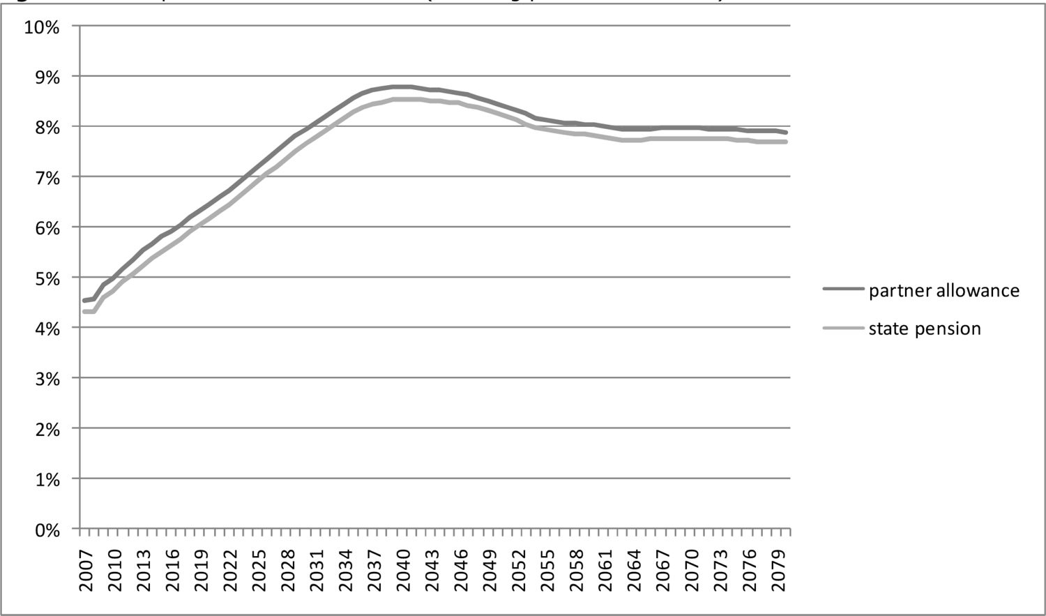
State pension cost as % of GDP (including partner allowances) 2009–2080.
In reality, of course pensions will increase in real terms, as GDP does. Van Ewijk et al. (2006) assume for the oncoming decades state pensions to increase by 1.7% a year in real terms and GDP to grow by 1.4% a year in real terms. If that assumption holds true, in terms of percentage of GDP, the state pension costs will rise from 4.8% in 2009 to 9.6% in 2040 as GDP grows more slowly than the state pensions in real terms.
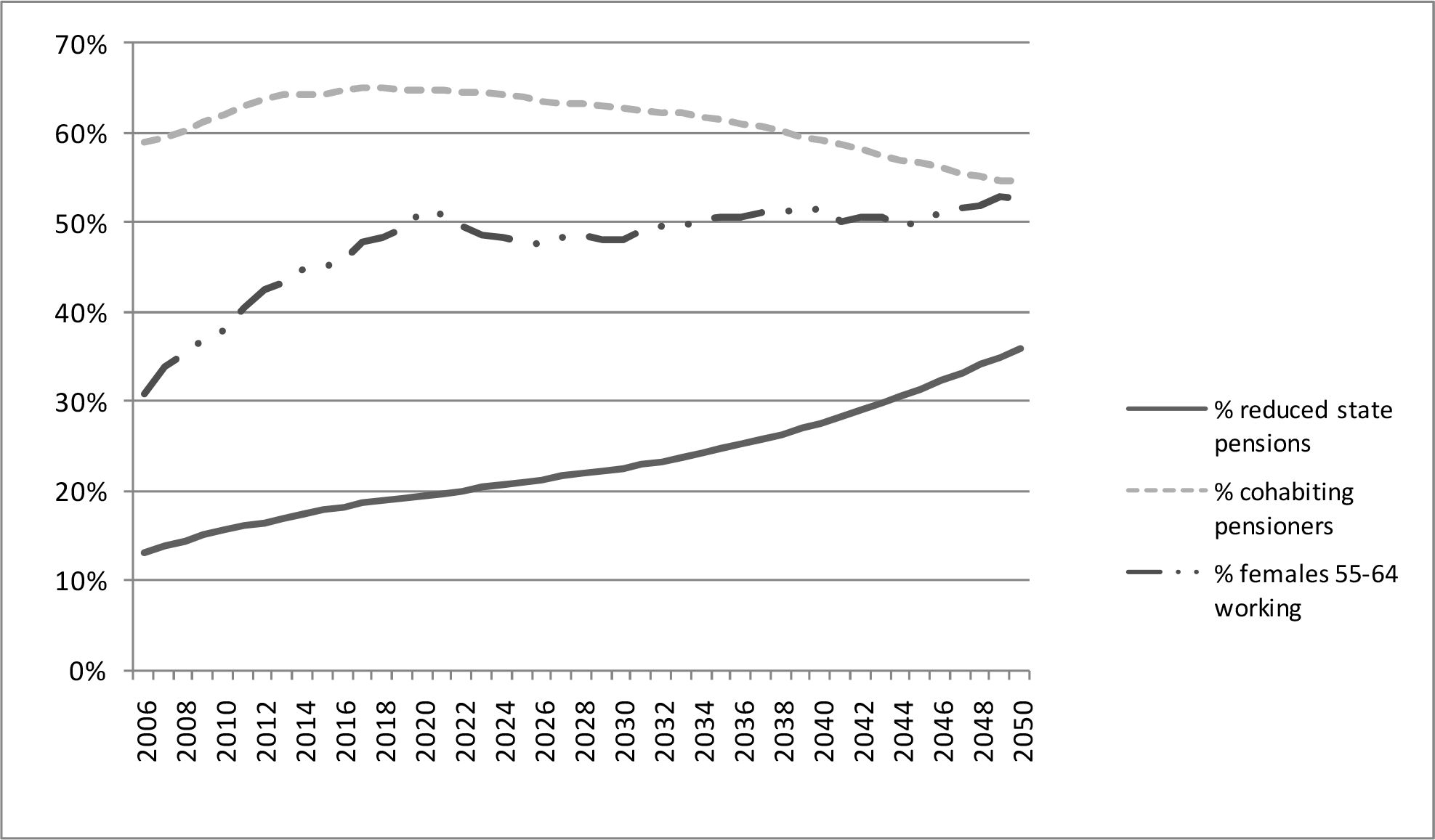
There are several reasons for the lower than expected rise of the state pension costs. From the simulation results, it appears that not only does the size of the population of pensioners change but that its composition changes as well. In particular, three trends are important. First, when studying the composition of the pensioner population by origin, it appears that the share of immigrants is rising. This holds true especially for the first generation immigrants. Their share in the population aged 65 and over almost doubles from 8.7% in 2009 to 15.6% in 2040. Most first generation immigrants have an incomplete state pension (unless they immigrated to the Netherlands before age 15). Emigrants will also have a reduced state pension and their number is growing as well. The number of reduced pensions is therefore rising, from 15.0% in 2009 to 27.5% in 2040.
The second is the development of the share of cohabitants in the pensioner population. This result is less clear-cut. In the short term the share of cohabitants among pensioners is increasing. This reflects the trend seen in recent state pension realizations and is caused by the increasing life expectancy. Partners live together for a longer time after reaching the age of 65. For the same reason, in a recent study by Poos et al. (2008), a decrease in health care costs is predicted for the forthcoming decade. However, after 2020 the percentage of singles starts increasing again. This can be explained by the socio-economic trend that fewer people become cohabitant or married. This trend finally overshadows the current trend of increasing numbers of cohabitants because of the rising life expectancy. Already in 2040, the share of single persons among pensioners is above the current level. After 2040 the share of singles will stabilize at a level above the current and put additional pressure on state pension costs.
A third important trend is the rising labour participation over time, especially among women. This influences the number of people qualifying for the partner allowance. These allowances currently account for € 1.4 billion. A person qualifies for the partner allowance when he or she turns 65 and has a partner who is younger than 65 and does not earn enough income of their own4. Most of those who qualify for the partner allowance are men. Men tend to have a wife who is on average three years younger, and labour participation among older women is still particularly low. In fact, the majority of men turning 65 currently qualifies for the partner allowance. However, as the labour participation among women is rising, this number will be decreasing in the future. Therefore, the costs of the partner allowances will grow slowly until 2013, then stabilize more or less on the same level and decrease slowly after 2035. In the meantime the share of women in the age category 60–64 who participate in the labour market will have doubled. In 2040 the costs of the partner allowance will be almost equal to 2009.
Figure 4 shows all three trends. In sum, the cost per person accounts for a reduction of state pension cost equivalent to 0.3% of GDP. The rising share of reduced state pensions, mainly because of the rising share of first generation immigrants and the rising labour participation of women each account for 0.2%. The development in the share of single persons in the population of pensioners has a small upward effect of 0.1% of GDP in 2040.

Changes in composition of pensioners population (2006-2050).
5.2. Redistribution
Redistribution within the scheme is investigated in detail by computing the share of lifetime state pension income taken by different subgroups. The lifetime state pension income is computed by accumulating incomes from the year a person turns 65 until the year a person dies. For this analysis, the 2006–2045 pensioner cohorts (the 1941–1980 birth cohorts) are aggregated. The average lifetime state pension income per person is around € 190,000, with lifetime income per person decreasing for the later cohorts because of the rising number of people with incomplete state pension entitlements. Table 3 shows a subdivision of the accumulated cohorts by subgroup, with the share of each subgroup in the cohorts of pensioners, its share of lifetime state pension income and the ratio between the two.
Share of lifetime state pension income compared to share of state pension cohorts.
| Subgroup | Share of cohorts turning 65 | Share of lifetime pension costs | Ratio |
|---|---|---|---|
| By income | |||
| - 1st quintile | 19.4% | 15.4% | 0.79 |
| - 2nd quintile | 19.8% | 18.5% | 0.93 |
| - 3rd quintile | 20.0% | 19.4% | 0.97 |
| - 4th quintile | 20.3% | 21.8% | 1.08 |
| - 5th quintile | 20.5% | 24.9% | 1.21 |
| By gender | |||
| - Women | 49.4% | 52.6% | 1.06 |
| - Men | 50.6% | 47.4% | 0.94 |
| By household status | |||
| - Singles | 30.6% | 34.0% | 1.11 |
| - Cohabitants | 69.4% | 66.0% | 0.95 |
| By origin | |||
| - Natives | 73.5% | 82.4% | 1.12 |
| - Immigrants | 26.5% | 17.6% | 0.66 |
The higher income quintiles receive an aboveaverage share of total state pension because of differences in life expectancy. This redistribution through life expectancy is substantial. The first income quintile receives more than a third less than the fifth income quintile (a ratio of 0.79 vs. a ratio of 1.21). This is mainly due to the difference in life expectancy, but also to the larger share of incomplete state pensions in the lower income quintiles. Women receive 6% more state pension from the scheme than their share in the cohort would justify. Singles receive 11% more state pension from the scheme than their share in the cohort would justify. This is because the lower life expectancy of singles is overcompensated by their higher state pension. Immigrants receive 34% less state pension from the scheme than their share in the cohort would justify. However, this large difference is primarily due to immigrants building up less entitlement during their life and only for a smaller part due to differences in life expectancy.
5.3. Retirement decision
The participation transitions after age 60 in SADNAP are modelled through the behavioural option value model described in Section 4. The participation rates at age 60 are given by the participation status model from appendix A.3 and are similar to the participation rates for people aged 60 as projected by CPB. The retirement decision is determined by the option value model only for those still working at age 60. This excludes about 40% of the cohorts as even in the long run some 30% of the men aged 60 and 50% of the women aged 60 will be in receipt of benefits or not participating in the labour market at all.
When the distribution of individual retirement ages is studied, we find spikes at certain pivotal ages. This is a well known phenomenon (e.g. Lumsdaine, Stock and Wise, 1995 and Gustman and Steinmeier, 2005) which can be partly explained by retirement taking place according to social-cultural norms, but also partly by economic reasons. As the models, like the option value approach we use, only take the latter into account, they usually underestimate the spikes. For the Netherlands, Nelissen (2002) finds a strong preference for individuals to retire either at the first or the last possible retirement age. In the Netherlands, the first possible retirement age used to be 60 years in many sectors. Since the late 1980s for most employees a generous early retirement scheme existed that guaranteed an income level of 70–80% of the final wage without loss of pension accruals from 60 years of age onwards. As a result, most people did indeed retire at age 60 (Euwals, de Mooij & van Vuuren, 2009). Gradually, the generous early retirement schemes are being replaced by actuarially neutral schemes until, from 2015 onwards, all schemes are fully actuarially neutral (Bovenberg & Gradus, 2008). The last possible retirement age in the Netherlands for most employees is still 65. At that age, the state pension starts being paid and most employees automatically have their employment terminated. However, the Dutch government has sent a proposal to parliament to abolish the automatic process of employees being fired at 65 and to allow delaying the state pension to 70 years of age instead of the current 65.
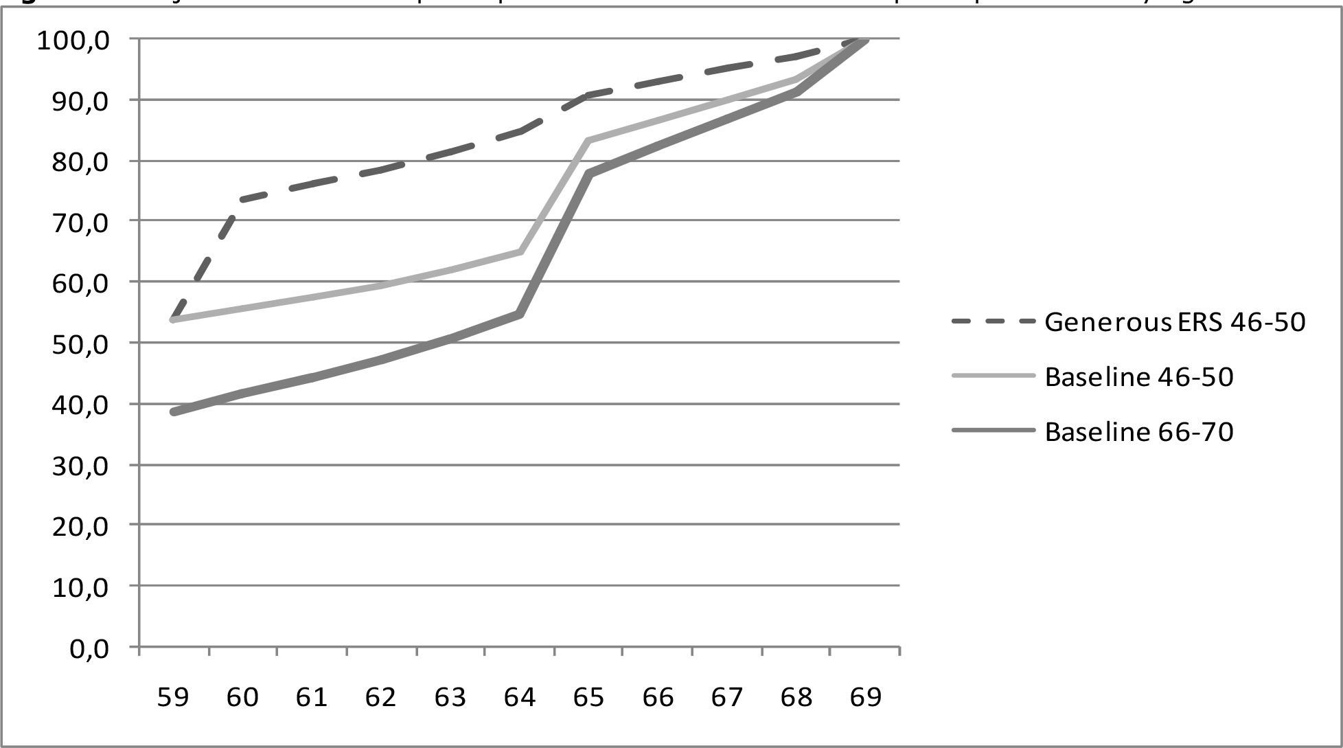
When the retirement decisions in SADNAP are evaluated, indeed, when the generous early retirement scheme is in place, the majority of retirement decisions takes place at 60, the earliest possible age. In a fully actuarially neutral scheme (assuming a last possible retirement age of 70), the model predicts two spikes in retirement, a large one at 65 and a smaller one at the last possible retirement age. The lines in Figure 5 show these retirement patterns. The dashed line gives the retirement pattern of the birth cohorts 19461950 (those that turn 60 between 2006 and 2010) when the generous early retirement scheme would still have been in place (assuming 80% of the working population to be covered by this generous ERS providing an income level of 75% of the wage at age 60). The solid line gives the retirement pattern of the same cohort in an actuarially neutral early retirement scheme. The average retirement age rises by 2.5 years for those who are working at least until 60 in the actuarially neutral scenario. The bold line gives the retirement pattern of the birth cohorts 1966–1970 (those who turn 60 between 2026 and 2030). The share of non/participants at age 59 decreases from 54% to 39% between those cohorts. The average retirement age for the entire population rises by one year (from 61,9 to 62,8) because of the higher number of people working at least until 60.

Projected rate of non-participation in the labour force non-participation rate by age.
The average retirement age increases with 2.5 years for the population still participating at age 60. Results in the same order of magnitude were found by de Vos and Kapteyn (2004), who simulated the effect of a change from the generous ERS that existed in the Netherlands at the time to a more or less actuarially neutral scheme. They forecasted an increase in average retirement age of four years for males and insignificant changes for women with the option value model, which in the same study they found to perform better than the peak value model in the baseline estimation. In 2007, retirement age had indeed increased by two years to 61.7 years from below 60 during the 1990s when the generous early retirement schemes were common (Advies Commissie Arbeidsparticipatie, 2008). However, even when the generous early retirement schemes were common, a fair share of workers continued working until 65 or later. This concerns mainly the self-employed and also employees not covered by collective agreements on early retirement. On the other hand, 40% of the population is no longer participating in the workforce at age 60, which still leaves important participation gains to be made.
The model predicts 26% of the people working at 60 to retire before 65, 38% to retire at 65 and the other 36% to retire past 65. Those retiring early are the ones with high time preference, high leisure preference or high expected wage decrease, or they are risk-averse, or a combination of the above. The influence of time preference and leisure preference seems to be dominant. Also, disability is an important factor causing early retirement for about one in six retirees who retire early. As the disability scheme in the Netherlands currently is so strict that abuse of the scheme as a means of early retirement is virtually impossible, the unemployment scheme is nowadays often used as an early retirement pathway at all ages. Table 4 gives a characterization of the retirees per retirement age:
Characteristics of retirees by retirement age (birth cohorts 1946–1970).
| Retirement age | Share of population retiring | Time preference | Leisure preference | Risk aversion | Wage decrease | Share of disability |
|---|---|---|---|---|---|---|
| ≤ 59 | 0.427 | |||||
| 60 | 0.029 | 0.26 | 2.15 | 0.70 | 0.046 | 0.14 |
| 61 | 0.025 | 0.21 | 2.07 | 0.70 | 0.046 | 0.16 |
| 62 | 0.027 | 0.20 | 2.04 | 0.70 | 0.046 | 0.17 |
| 63 | 0.035 | 0.21 | 2.04 | 0.70 | 0.047 | 0.14 |
| 64 | 0.036 | 0.21 | 2.07 | 0.70 | 0.048 | 0.18 |
| 65 | 0.217 | 0.20 | 2.05 | 0.69 | 0.046 | 0.03 |
| 66 | 0.043 | 0.14 | 1.97 | 0.70 | 0.046 | 0.14 |
| 67 | 0.042 | 0.13 | 1.97 | 0.71 | 0.046 | 0.15 |
| 68 | 0.040 | 0.12 | 1.94 | 0.71 | 0.045 | 0.14 |
| 69 | 0.080 | 0.08 | 1.81 | 0.73 | 0.039 | 0.06 |
The SADNAP model rightly predicts a strong preference for retiring at 65, the year the state pension (and partner allowance) start being paid. However, the number of people working on past 65 is slightly higher than the levels currently seen, especially for women. The abolition of the automatic termination of employees at 65, which is expected soon, will probably influence current retirement patterns. Moreover, it is known (Coile, 2004) that husbands’ and wives’ retirement behaviour is influenced not only by their own financial incentives but also by spill-over effects from their spouses’ incentives, which may explain why women’s retirement age is overestimated by the option value algorithm. The SADNAP estimates may give a good estimate of the retirement patterns that will be realized when the automatic firing of employees at 65 has been abolished and when all early retirement schemes that are rewarding early retirement are abolished. However, it remains to be seen whether such a substantial part of the whole population of males and females will retire at the last possible retirement age when that last possible retirement age is increased to 70.
5.4. Validation and comparison to other models
The demographic model results are benchmarked with the official population forecast of the CBS. The SADNAP estimates in all years stay within a margin of 1% of the comparable CBS estimates for main age groups. There is no exact match with macro population numbers as only the yearly number of births and immigrants and mortality and emigration rates are aligned to CBS forecasts. The grey pressure, a key indicator, equals 49% in 2040 in both SADNAP and the CBS-projection.
The financial forecast compares well to the earlier macro calculations of Van Ewijk et al. (2006), who forecasted a rise in state pension cost from 4.7% of GDP in 2006 to 8.8% of GDP in 2040, based on the 2004 population forecast of CBS. As in the 2008 population forecast the number of people aged 65 and over in 2040 is 12% higher than in the 2004 forecast, an update of the calculations of van Ewijk et al. based on the newest population projection would lead to an estimate of 9.9% of GDP in 2040. The difference with the 9.6% is caused by the decreasing cost per person that was not taken into account in the macro approach.
The short-term forecast of number of state pensioners and state pension costs gives comparable results for 2009. The number of pensioners is 0.6% lower than the 2009 estimate of SVB, the pension administration office. In later years the SADNAP estimates point to slightly higher state pension costs and a slightly higher number of state pensioners. In 2024, the last year of the SVB forecast, the number of pensioners is 0.2% higher than the SVB estimate.
Recent studies report mixed findings on whether people actually reach their target of a 70% replacement rate (total pension as a percentage of the final wage). Statistics Netherlands (CBS, 2008) finds that a gross income level of on average 73% of the final wage is to be expected for the cohorts currently saving for their pension. The SADNAP results show the same average replacement rate. Moreover, in a micro simulation study on the wealth of Dutch pensioners (SZW, 2006) the income position of pensioners is found to improve substantially as a consequence of more second and third-pillar pension savings by younger generations. The researchers show the average net income of the 65–69 years olds to rise to 102% of the income of the 60–64 years olds in 2030 as compared to 92% in 2010. Knoef, Alessie and Kalwij (2009) also report that between 2008 and 2020 mean equivalised household income increases by 11–14% for the retirees. However, Euwals, de Mooij and van Vuuren (2009) find that when the consequences of the career average system to which most pension funds have recently switched are taken into account, the younger generations have lower replacement rates, up to less than 50% for the birth cohorts 1972–1976 (weighted average of all cohorts 64%). The SADNAP results show rising replacement rates and are in line with the estimates of SZW and Knoef, Alessie and Kalwij.
Few comparable studies are available on redistribution. Knoef, Alessie and Kalwij (2009) report a Gini-coefficient of 0.23 for the population of retirees, based on equivalised household income. This is well below the Gini-coefficient of 0.29 as reported by SADNAP, which is based on individual income. However, a lower Gini-coefficient when comparing household income is plausible because higher income earners (mainly males) usually have younger partners, so their income will generally be shared with a partner, decreasing the level of inequality measured.
The average retirement age increases by 2.5 years as compared to the benchmark scenario of a generous early retirement system. Results in the same order of magnitude were reported by de Vos and Kapteyn (2004), as described in section 5.3, and Euwals de Mooij and van Vuuren (2009). Table 5 gives an overview of some key SADNAP results and some comparable estimates.
Overview of key SADNAP results compared to other models.
| Indicator | Year | SADNAP estimate | Comparable estimate | By |
|---|---|---|---|---|
| Grey pressure | 2040 | 49% | 49% | CBS |
| State pension expenses | 2040 | 9.6% | 8.8% | CPB based on 2004 population projection, would be 9.9% based on 2008 population projection |
| Number of state pensions | 2024 | 4.132 mln | 4.125 mln | SVB 2009–2024 projection |
| Expected replacement rate when retiring | All | 0.73 | 0.73 0.64 | CBS Euwals, de Mooij, van Vuuren (2009) |
| Gini coefficient | 2040 | 0.29 | 0.23 | Knoef et al. on household income (SADNAP estimate on individual income) |
| Retirement age | 2007 | 61.9 | 61.7 | Adviescommissie Arbeidparticipatie (2008) |
| Retirement age increase (compared to generous ERS) | 2015 | 2.5 | 4 / 0 2 – 2.5 | De Vos and Kapteyn for men / women Euwals, de Mooij, van Vuuren (2009) |
6. Conclusions and topics for future research
Like most other OECD countries, the Netherlands is facing an ageing population, causing a burden on the public finances. A significant part of the rise in public expenses will be caused by the rise in costs for the state pensions. The old-age dependency ratio almost doubles from now until 2040 (the peak of the ageing process in the Netherlands).
The dynamic population micro simulation model SADNAP is developed for calculating the financial and economic implications of the ageing problem and of the relevant policy measures considered. The model uses administrative datasets on state pension payments, state pension entitlements and private pension entitlements. Life paths are constructed for a sample of the Dutch population, including immigration and emigration, household formation and labour participation. In this paper, two extensions of the model are elaborated. First, because of improvement of the income data sources and differentiation of mortality rates, redistribution within the pensions system can be analysed. Second, the retirement decision is modelled based on the Stock and Wise option value approach, allowing for individual variation in the main option value parameters based on literature review in order to make use of the added value of micro simulation.
It is shown that in the baseline scenario the state pension costs rise less sharply than the number of pensioners. The composition of the pensioner population is changing. The number of immigrants with reduced state pensions is rising. During the forthcoming decades, the proportion of single persons among the pensioner population is decreasing, however, this trend will be reversed in the future. Also the rising labour participation of women decreases the cost of partner allowances. The downward influences together amount to 0.3% of GDP in 2040. This partly compensates for the increasing longevity from the latest population forecast.
The intra-generational redistribution within the Dutch pension scheme is shown to be substantial. The bottom income quintile receives less out of the system, a discount of more than one-third, than the top income quintile, mainly because of lower life expectancy. Singles, however, get more out of the system than partners in a couple. Their higher pension compensates for their shorter life expectancy.
The modelling of the retirement decision through the option value model confirms the retirement patterns experienced in the Netherlands when a very generous early retirement scheme was still in place. Average retirement age for those who are still working at 60 can rise by 2.5 years when the early retirement schemes have become fully actuarially neutral. In the actuarially neutral scheme, a strong preference for either retiring at 65 or at the last retirement age is suggested. The time preference and leisure preference parameters appear to be the most important drivers for the retirement decision. An assumption of wage decrease is added to the model in order to obtain more plausible results and less people working on until the last possible retirement age. Another important factor is the role of disability and unemployment. The unemployment scheme especially is still used as an early retirement pathway.
Future research will focus on evaluating policy options with the model. New datasets on state pensions and private pensions will become available for more recent years and more information on third-pillar pensions and financial wealth will become available on the micro level. Also, the availability of linkable datasets of different years will allow for an estimation of the option value parameters and their distribution.
Footnotes
1.
The gross minimum wage in 2009 amounts to approximately € 18,000 per year. The gross AOW-benefit for a single person is approximately € 12,700, the gross AOWbenefit for a couple is approximately € 8,700 for each partner. In net terms this amounts to 70% and 50% of the net minimum wage respectively.
2.
With some exceptions: benefits for the permanently, fully disabled equal 75% of the former wage during the first two months of unemployment and 70% for the three years thereafter. After those three years and two months, all people who become unemployed from age 60 onwards can claim a minimum benefit to bridge the gap until retirement at 65.
3.
In the Netherlands, the unemployment benefit currently lasts for a maximum of five years for people aged 60 and over. The unemployment benefit itself lasts for a maximum of three years and two months and the subsequent benefit for people aged 60 years and over complements the time until retirement.
4.
When the partner earns an income below 15% of the minimum wage, a full partner allowance of up to 50% of the minimum wage is given. When the partner earns an income between 15% and 97.5% of the minimum wage (SVB, 2008), a reduced partner allowance is given. When the partner earns more than 97.5% of the minimum wage, no allowance is granted anymore.
5.
In the Netherlands, the state pension system treats (formal) cohabitation in the same way as being married
6.
Including non-natives of the second generation (born in the Netherlands).
7.
In 2005, the maximum state pension for a single person was € 11,211 and for a partner in a couple € 8,008.
8.
The average replacement rates are higher than the median replacement rates, but they are not a good indicator as some people with high pension savings and very low wages (for example, because they worked for only part of the year) can have very high replacement rates.
The SADNAP Model
This appendix gives a more detailed description of the SADNAP model. The model is programmed in SAS and consists of different modules on demographics, household formation, labour participation and the retirement decision, which are described subsequently in Sections A.1 to A.3.
A.1 The demographic model
Before the simulation starts, a base data file is created out of the source files described in Section 3. Three different data sources are combined into a single file containing a representative sample of the Dutch population in the base year (2006). Aggregate CBS data on the population aged 0–15 years are used in the base year. For the population aged 15–64 years, the micro datasets from CBS on state pension entitlements and private pension entitlements as described in Section 3.2 are used. Finally the micro dataset from SVB on state pension payments as described in Section 3.1 is used for the population aged 65 and over. These three datasets complete the population for the base year. The records for people younger than 15 years are constructed by using general demographic CBS statistics on the age, gender and ethnic composition of the Dutch population. As state pension entitlements are zero until persons turn 15, and children do not have wages or private pension entitlements, no additional information on this group is needed.
The CBS file with entitlement data for people aged 15–64 has another year of origin (namely 2005) than the SVB file with payment data for people aged over 65 (namely 2006). Therefore, the 2005 population aged 15–64 is simulated towards a population aged 16–65 in 2006. A population can change by four demographic events; births, deaths, immigration, and emigration. Births do not affect the population aged 15–64 in one year of simulation. Therefore, the 2005 population is made subject to mortality, immigration, and emigration. After this first simulation the 2005 population is aged 16–65. Because richer data are available for people aged over 65 in 2006, persons aged 65 are deleted from the simulation. All age groups are added together to complete the base dataset.
For each simulation year, records for the new births and the new immigrants are added, based on the macro data sources as described in Section 3.3. When applying the mortality rates and emigration rates as derived from the CBS population projection, an accurate population forecast results. Stocks, flows and rates from the CBS are available until 2050. After 2050, the 2050 numbers are kept constant.
Although there is now an accurate population forecast, there is still a problem left relating to the complexity of the modelling of immigration and emigration. Also “remigration” needs to be modelled. This is important because on average during the last few years about 50% of the emigrants are former immigrants and about 20% of the immigrants are former emigrants. By not allowing for remigration, the share of immigrants in the population will clearly be overestimated. The former (immigrants having a greater emigration rate) can easily be implemented by using different sets of emigration rates depending on whether the emigrant was born in the Netherlands or not. The latter is more difficult. Few of the larger simulation models, notably Lifepaths and Sesim (Pennec & Keegan, 2007) allow for emigrants re-entering the population. SADNAP ignores repatriation of emigrants, resulting at the micro level in a slight overrepresentation of small entitlements as returning emigrants continue building up their already existing rights, whereas SADNAP assumes these rights to consist of separate parts belonging to two separate persons.
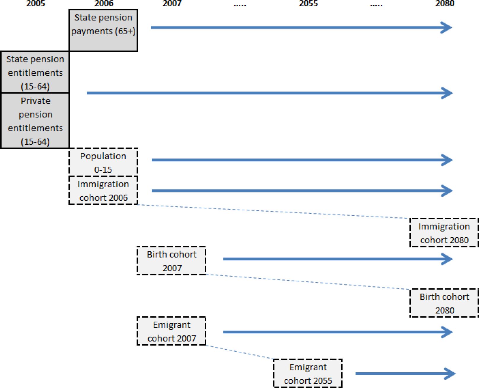
Moreover, still missing is a part of the population that will be entitled to a state pension in the future, but is not living in the Netherlands anymore. As can be seen from Table 1, 9% of the current population of pensioners is living abroad. Since emigration is modelled, the model captures all future pensioners who live in the Netherlands in the base year, but will emigrate in the future. However, we still miss the people aged between 15 and 64 in the base year who built up state pension entitlements in the Netherlands in the past but emigrated before the base year. To correct for this, records are added for former emigrants. As a starting point, the youngest cohort of pensioners in the base year is used. Of this cohort also 9% of the pensioners are living abroad. From the state pension entitlement, their year of emigration can be estimated. Everybody missing one year of entitlement is assumed to have emigrated at age 64, everybody missing two years at age 63 and so on. As in the simulation, people aged 64 in the base year can emigrate in the first year of the simulation, after that first year of the simulation only the claimants living abroad who emigrated at age 63 or younger have to be added. According to SVB (2008), non-take-up among people living abroad is common, hence a correction is made, based on the assumption that the younger one emigrated, the less likely one is to claim a Dutch state pension.
The whole process described above is represented in Figure 6. The filled boxes represent the micro databases from the base years that are used in the simulation and the blank boxes represent the micro data that are constructed from macro data sources in order to add new cohorts to the base year data.

The simulation process of the population forecast.
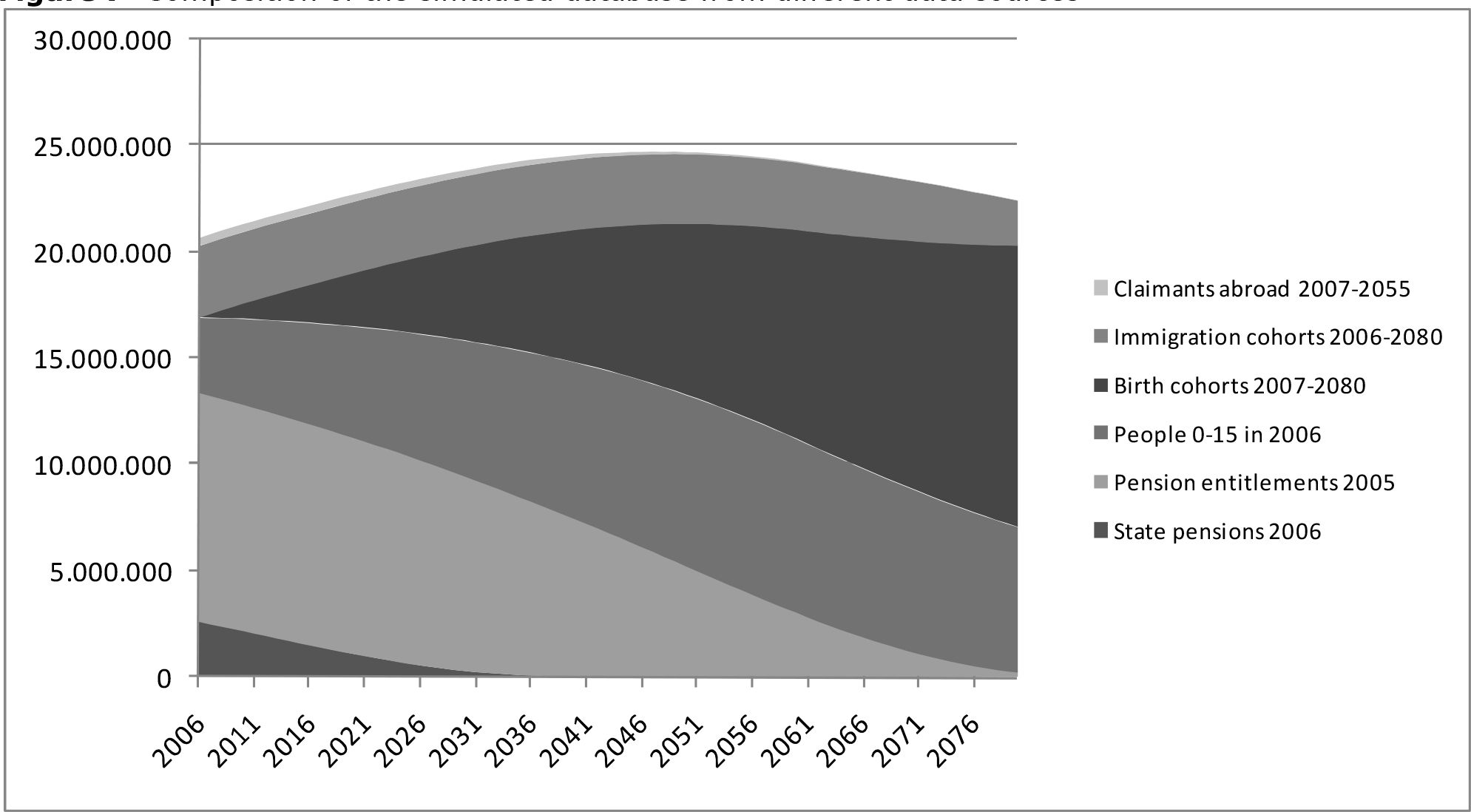
Figure 7 shows the composition of the simulation database, based on a 1% sample and extrapolated to the whole population. The numbers add up to more than the population of the Netherlands as the life paths of immigrants are taken into account before they immigrate to the Netherlands and the life paths of emigrants are taken into account after they leave the Netherlands. In 2080, the final year of the simulation, the base year micro data sets will almost completely have phased out and will have been replaced by persons from the constructed datasets from 2006 onwards.

Composition of the simulated database from different data sources.
A.2 The household formation model
In the next steps variables are added to the demographic model, such as household type. From the databases of pension entitlements and pension payments, the household status of all individuals aged 15 and over is known. SADNAP distinguishes between single persons and cohabitants only5. The aggregated state pension for two singles is higher than the aggregated state pension of two partners in a couple.
Age- and gender-dependent transition probabilities are used to determine whether single persons remain single or start cohabiting and whether cohabitants separate and become single or stay together. The transition probabilities can be derived from the age- and gender-specific household forecast from CBS as described in Section 3.3.
When PS denotes the probability of being single and PC the probability of cohabiting, the transition probabilities PSC (probability of a single person cohabiting the next year) and PCS (probability of a cohabitant being single again the next year) can be defined as follows:
If the correction terms £(age, gender) are set to zero, most individuals will have only one lasting relationship during their lifetime. The higher the correction terms are set, the more relationships will be started and finished each year. The correction terms can be used to align the simulation to the information on household formation and dissolution from the CBS household forecast. In the baseline scenario, the terms are set to zero.
However, by introducing differences in mortality rates (see Section 3), a deviation is introduced from the original population projection in the numbers of singles and cohabitants by age. As the household formation model from appendix A.2 is based on the original population projection, the numbers need to be realigned in order to match the original population projection again. Concretely, the equations (3) and (5) need to be adapted as the probabilities of singles cohabiting need to decrease and the probabilities of cohabitants becoming single again need to increase.
In some larger micro simulation models, the cohabiting process is very elaborate. Those models contain a formalized mate matching module in which partners are found within the model based on certain matching criteria (for an overview of methods see Perese (2002) and for an overview of models see Bacon and Pennec (2007)). SADNAP follows a simple approach, in which the important characteristics of the partner are determined as soon as those characteristics become relevant for the model calculations. In the ageing calculations the gender, age and participation status of the partner are the most important characteristics. The gender of the partner is assumed always to be the opposite of the gender of the other partner. From the dataset of state pension payments, detailed information on the age difference between partners of a couple is available. The age differences from the youngest cohort of this dataset (the 1941 birth cohort) are used, assuming that the distribution of age differences in relationships will remain the same in the future. Given the gender and age of a partner, the corresponding participation rate can be derived from the age and gender specific participation estimates as described in Section 3.3. At this point enough information is available to calculate the costs of the state pension. Information is available on the future population size and its division by ages. Starting with current state pension entitlements, the building up of entitlements in the future can be simulated. As information on the household type is also available, by adding benefit levels to the model, the future state pension benefits of all individuals can be simulated. The total costs for the state pension can be calculated by aggregating the individual benefits. All calculations within the model are done at the current price level.
A.3 The participation status model
From the database of pension entitlements, the labour market status of all individuals aged 15 to 64 is also known. Participants can be either employees or self-employed. The self-employed, for whom we have no data on private pension savings, are treated by assuming their pension savings on average to be equal to those of the employees. Non-participants can be either studying, receiving a benefit, early retired or not participating at all. Figure 8 shows the distribution of the 2005 Dutch population by age and by participation category.

Composition of the 2005 population by age and participation category.
One of the most striking conclusions from the above graph is that in the last couple of years before the statutory retirement age of 65, only a small minority of the population is still working. This is mainly due to the popularity of early retirement schemes and the use of benefits, especially disability and unemployment, as an early exit route (see e.g. Kapteyn and de Vos, 2004). For example, of the 64 year olds, only 11% are working, whereas 27% are on benefit and 39% are early retired. However, the participation rate among the 60–64 years old is currently rising due to policy changes, especially regarding early retirement schemes and disability insurance (Euwals, de Mooij & van Vuuren, 2009).
In SADNAP, age and gender dependent transition probabilities are used to determine whether participants continue participating or become nonparticipants, and vice versa. The transition probabilities can be derived from the age- and gender-specific forecast of participation rates from CPB as described in Section 3.3. Participation in SADNAP is a binary state. Participants include employees, the self-employed and the involuntarily unemployed who are actively seeking work. Non-participants are not available to the labour market and include students, disability benefit recipients, the early retired and the voluntarily unemployed.
When PN denotes the probability of being nonparticipating and PP the probability of participating, the transition probabilities PNP (probability of a non-participant participating the next year) and PPN (probability of a participant not participating the next year) can be defined as follows:
Again, if the correction terms £(age, gender) are set to zero, most individuals will have only one uninterrupted period of participation during their lifetime. The higher the correction terms are set, the more short periods of participation and nonparticipation will occur during a life-course. In the baseline scenario, the terms are set to zero. The transition probabilities are used only until people turn 60. From that age on, the retirement decision (for those who are still participating at age 60) is modelled through the behavioural option value model as described in Section 4.
Data sources
B.1 State pension data
From the state pension perspective the Dutch population can be separated into three groups; people aged younger than 15, people aged between 15 and 64, and people older than 65. People younger than 15 are not yet building up state pension rights. People between 15 and 64 are building up those rights when living in the Netherlands, and people aged 65 plus are receiving a state pension if they have built up entitlements in the past. For the latter two groups micro data files are available.
Two institutions provide the micro data sources. Statistics Netherlands (CBS) supplies a micro data file concerning state pension entitlements. This file contains all of the over 11 million persons aged 15–64 who live in the Netherlands. Variables in this dataset include birth date, nation of origin, gender, household status, and the number of entitled years for the AOW. Micro datasets are available for 2004 and 2005.
The Social Insurance Bank (SVB) is the authority that accomplishes the payment of, among others, state pensions. The Ministry of Social Affairs and Employment receives detailed data from the SVB on the current state pensions, including a full administrative data file with information on all 2.6 million persons that were receiving AOW in 2006. The SVB data file contains information on gender, birth date, country of residence, marital status, birth date of the partner, number of entitled years for the AOW and entitlement to a partner allowance. Moreover, this file contains information on people receiving AOW abroad whereas the CBS only delivers AOW information on inhabitants of the Netherlands. Some characteristics of the two main data sources can be found in Table 6.
Some characteristics of the two main data sources on state pensions.
| SVB file 2006 (65+) | CBS entitlement file 2005 (15-64) | |||
|---|---|---|---|---|
| Number | % | Number | % | |
| Gender | ||||
| - Male | 1,130,506 | 43.5 | 5,563,649 | 50.5 |
| - Female | 1,469,568 | 56.5 | 5,458,248 | 49.5 |
| Origin | ||||
| - Native6 | 9,656,948 | 87.6 | ||
| - Immigrant (1st gen) | 1,364,949 | 12.4 | ||
| Household status | ||||
| - Single | 2,667,713 | 24.2 | ||
| - Cohabiting | 8,337,017 | 75.8 | ||
| State pension entitlement | ||||
| - Complete | 2,200,342 | 84.6 | 9,443,153 | 85.7 |
| - Reduced | 399,802 | 15.4 | 1,572,768 | 14.3 |
| Country of residence | ||||
| - Netherlands | 2,364,891 | 91.0 | ||
| - Abroad | 235,183 | 9.0 | ||
| Total | 2,600,074 | 100.0 | 11,021,897 | 100.0 |
Because of their higher life expectancy, women outnumber men by 56,5% to 43,5% among the population aged 65 and over. Among the population of 15–64 year olds, however, men outnumber women by 50.5% to 49.5%. Over 12% of the population aged 15–64 are first-generation immigrants (not born in the Netherlands). Among this group, reduced AOW rights are common because the majority of the group migrated to the Netherlands after the age of 15. Almost 15% of the population aged 15–64 already has a reduced right. This is about the same as the share of reduced rights among the current population of pensioners, but this percentage will rise in the future because before reaching the age of 65, part of the population aged 15–64 who at the moment have a complete entitlement can lose some years of accrued rights when they go abroad.
B.2 Company pension data
Recently, Statistics Netherlands has also started providing micro data on (second-pillar) company pensions. In 2009, a micro dataset became available based on data of a representative sample of pension funds including the large pension funds for civil servants and health workers. This file includes individual data on company pension entitlements of 53% of the population aged 15–64 and 67% of the Dutch employees. Some characteristics of the data source on private pension entitlements can be found in Table 7.
Some characteristics of the main data source on company pensions.
| State pension entitlements | Private pension entitlements | |||
|---|---|---|---|---|
| Number | % | Number | % | |
| Gender | ||||
| - Male | 5,563,649 | 50.5 | 3,151,280 | 54.2 |
| - Female | 5,458,248 | 49.5 | 2,664,918 | 45.8 |
| Origin | ||||
| - Native | 9,656,948 | 87.6 | 5,288,526 | 90.9 |
| - Immigrant (1st gen) | 1,364,949 | 12.4 | 527,672 | 9.1 |
| Household status | ||||
| - Single | 2,667,713 | 24.2 | 1,325,328 | 22.8 |
| - Cohabiting | 8,337,017 | 75.8 | 4,484,873 | 77.2 |
| State pension entitlement | ||||
| - Complete | 9,443,153 | 85.7 | 5,074,905 | 87.3 |
| - Reduced | 1,572,768 | 14.3 | 739,206 | 12.7 |
| Participation status | ||||
| - Study | 1,207,782 | 11.0 | 128,824 | 2.2 |
| - Work | 6,916,620 | 62.9 | 4,474,776 | 76.9 |
| - Benefit | 1,320,852 | 12.0 | 644,887 | 11.1 |
| - None | 1,217,069 | 11.1 | 318,848 | 5.5 |
| - (Early) retired | 342,141 | 3.1 | 246,483 | 4.2 |
| Total | 11,021,897 | 100.0 | 5,816,198 | 100.0 |
As can be seen from comparing the figures for state pensions and private pensions, the distribution of the main characteristics differs somewhat between the full set of people aged 15 to 64 and the subset of those whose private pension entitlements are also surveyed. This is caused by some people having no second-pillar pension entitlements at all, like students, selfemployed, people on social assistance and people who have never worked or who work in low-wage jobs without building up entitlements.
Besides the common characteristics like gender, birth date, ethnicity and household status, the data set contains a projection of the expected private pension if a person’s career is continued with the same wage as in 2005. This means that the older a person is, the more accurate the forecast will be, especially since most pension funds in the Netherlands changed to a career-average pension instead of a final-salary pension around 2004. The average wages, expected pensions and median replacement rates (expected state pension + expected private pension/wage) by subgroup are presented in Table 8. They concern the almost 4,2 million employees and exclude the self-employed, who usually build up their own pension savings in the third pillar.
Expected private pension by main subgroups.
| Wage (mean) | Expected private pension (mean) | Expected replacement rate (median) | |
|---|---|---|---|
| Age-category | |||
| - 15-19 | € 12,546 | € 3,740 | 1.283 |
| - 20-24 | € 20,605 | € 7,005 | 0.857 |
| - 25-29 | € 25,580 | € 9,128 | 0.779 |
| - 30-34 | € 28,623 | € 10,445 | 0.754 |
| - 35-39 | € 30,294 | € 11,323 | 0.747 |
| - 40-44 | € 31,855 | € 12,194 | 0.729 |
| - 45-49 | € 33,582 | € 13,020 | 0.702 |
| - 50-54 | € 34,911 | € 13,668 | 0.675 |
| - 55-59 | € 36,016 | € 12,460 | 0.638 |
| - 60-64 | € 36,594 | € 10,335 | 0.575 |
| Gender | |||
| - Male | € 37,892 | € 13,965 | 0.644 |
| - Female | € 21,984 | € 8,275 | 0.839 |
| Origin | |||
| - Native | € 31,008 | € 11,714 | 0.743 |
| - Immigrant | € 27,282 | € 7,791 | 0.607 |
| Household status | |||
| - Single | € 28,989 | € 9,952 | 0.761 |
| - Cohabiting | € 31,147 | € 11,767 | 0.725 |
| State pension entitlement | |||
| - Complete | € 30,536 | € 11,628 | 0.751 |
| - Reduced | € 32,062 | € 9,484 | 0.576 |
| All | € 30,703 | € 11,394 | 0.732 |
When interpreting the data, we see familiar patterns like wages and pension entitlements rising with age and men, natives and cohabitants having considerably higher wages and pensions than women, immigrants and single persons respectively. On average, employees have expected second-pillar pension savings of € 11, 394 which is more than the expected state pension savings7. The data confirm the growing importance of company pensions as an income component of the elderly.
The expected private pension peaks in the age category 50–54. Past that age, decreases are most probably due to people with high pension savings tending to retire earlier, although it is also known that the younger cohorts tend to have higher second-pillar pension savings (SZW, 2006). Also, there is a correlation between first and second pillar pensions. People with high company pensions more often have a complete state pension, whereas people with incomplete state pension entitlements more often have smaller or no company pensions. Rather surprising though, is that people with reduced state pension entitlements tend to have higher wages than people with complete entitlements. However, this only holds true for the population of employees, 7 In 2005, the maximum state pension for a single person was € 11,211 and for a partner in a couple € 8,008. which indicates that people who have lived abroad for a while tend to have higher than average wages. For the general population, immigrants with reduced state pension entitlements tend to be on benefits more often.
The median replacement rate8 is 0.73, but there are sizeable differences between subgroups with women, natives and singles having higher replacement rates than men, immigrants and cohabitants respectively. The high replacement rates of women are due to the large share of women in the Netherlands who during their life-course change to part-time jobs whereas pension savings up till then may have been based on fulltime jobs. The higher replacement rates of singles are due to the higher first pillar state pension for which they qualify. The replacement rates tend to decrease by age. This is partly due to younger cohorts having higher second-pillar pension savings, although it should be kept in mind that in a career average system, replacement rates will go down with age as wages tend to grow with age and replacement rates are related to the final wage. Also the very high replacement rates among the youngest age groups need explanation. In the Netherlands a full minimum wage can only be earned at 23 years of age. Wages paid to workers below that age tend to be lower, whereas expected private pensions take account of the wage increase due to legal requirements. But because major career jumps have yet to take place at that age, the expected private pensions for the younger cohorts are not reliable indicators anyway.
Statistics Netherlands is currently preparing a micro dataset on (third-pillar) individual arrangements, based mainly on data files from insurance companies. This dataset is expected to be available to researchers in 2009. These data are especially important for groups that cannot participate in the company pension schemes, like the self-employed. Finally, Statistics Netherlands is preparing a micro dataset on personal wealth, the so-called fourth pillar from tax office databases. This fourth pillar is known to play a role in the retirement decision (Bloemen, 2008) and can also be particularly important when intergenerational wealth transfers are researched.
B.3 Macro data sources
In SADNAP, some macro data sources are also used. On demographic events, the most recent population projection by age, gender and ethnicity by Statistics Netherlands (CBS, 2009) is used. From this projection, which runs from 2008 to 2050, we take the number of births and the number of immigrants by age and gender per year. Also mortality rates and emigration rates by age and gender are deducted from this projection. Although this official projection is used in the baseline scenario, by including the underlying processes of emigration, immigration, births and deaths, the model allows for analyses of alternative scenarios in which (policy-driven) changes, for example, in immigration or emigration levels can be represented. In SADNAP, a narrow definition of ethnicity is used, distinguishing only between natives and immigrants (people not born in the Netherlands) as distinguishing between second generation nonnatives and natives is not important for the state pension entitlements.
Information on household types is available for the most recent population projection. From this projection, which runs from 2009 to 2050, the cohabiting rates by age and gender are derived. The CBS data distinguish between single persons, couples, lone parents, children living with their parents, people living in institutions and a remainder group of people cohabiting without having a relationship to each other (e.g. students). In SADNAP only single persons and cohabitants are distinguished, based on the social benefits for which they qualify. The remainder group – people living together without having a relationship – are considered to be single persons. Of the people living in institutions, half are considered to be single and half to be cohabiting.
On labour participation, the most recent labour participation rates as provided by The Netherlands Bureau of Economic Policy Analysis (Euwals & Folmer, 2009) are used. These are average participation rates for five-year age classes by gender. From these five-year averages, participation rates for individual ages can be deducted. These participation rates include all persons who are available to the labour market, including the involuntarily unemployed who are actively seeking work. The non-participants are mainly students, disability benefit recipients, the early retired and the voluntarily unemployed (e.g. housewives). SADNAP currently lacks a model of benefit use during the life course. However, benefit use plays an important role in determining the net effects of ageing-related policy measures, like raising the retirement age. Therefore, in SADNAP the final state of benefit use at the age of 64 is modelled. It is assumed that benefit use at that high ages is an absorbing state (outflow rates are near zero). In 2005, based on the CBS dataset, 27% of the 64 year olds were in receipt of benefits: 17% from the disability insurance scheme, 2% from the unemployment insurance scheme, 4% from social assistance and 4% from other benefits. Because of the major reform of the DI scheme, the use of disability benefits will decline in the future. Long-term disability rates are based on current long-term forecasts based on the model described in Van Sonsbeek and Gradus (2006). In the meantime, the unemployment scheme has also undergone major reforms, limiting the duration of the benefit from a maximum of 7.5 years in 2003 to a maximum of just over 3 years in 2006. However, as Euwals, de Mooij and van Vuuren (2009) conclude that, as a result of the reforms of DI and early retirement schemes, pressure on UI may increase in the near future, it seems plausible to keep long-term rates for the other benefits constant at the 2005 level.
presents an overview of the macro data sources used.
| Age | Gender | Ethnicity | Household status | Participatio n status | Income | |
|---|---|---|---|---|---|---|
| Birth cohorts | n/a | E | E | n/a | n/a | n/a |
| Immigrant cohorts | E | E | E | - | - | - |
| Mortality rates | E | E | I | I | - | I |
| Emigration rates | E | E | E | - | - | - |
| Cohabiting rates | E | E | - | n/a | - | - |
| Participation rates | E | E | - | - | n/a | - |
| Benefit rates | E | E | - | - | E | - |
In Table 9, ‘E’ means that a characteristic is explicitly known from the data source itself, ‘I’ means that a characteristic is implicitly taken account of in the model and ‘-’ means that a characteristic is not known or used. Finally, some combinations, like the age and household status of newborns, are not applicable (n/a).
Baseline results
Forecasting accuracy for year 2000.
| Pension cost (× € 1 mln.) | Pensioners population (× 1,000) | Working population (× 1,000) | ||||||||
|---|---|---|---|---|---|---|---|---|---|---|
| State pension | Partner allowance | Total pension cost | Total cost as %GDP | Number of pensioners | % reduced pensions | % cohabitants | Working population | %particip. | % particip. Fem. 55–64 | |
| 2009 | 26,363 | 1403 | 27,765 | 4,85% | 2,748 | 15,0% | 61,3% | 7468 | 74,7% | 36,9% |
| 2010 | 27,087 | 1,444 | 28,532 | 4,98% | 2,843 | 15,5% | 61,9% | 7461 | 74,9% | 37,9% |
| 2011 | 28,024 | 1,535 | 29,559 | 5,16% | 2,965 | 15,9% | 62,9% | 7,436 | 75,2% | 40,5% |
| 2012 | 29,011 | 1,640 | 30,651 | 5,35% | 3,074 | 16,4% | 63,6% | 7,419 | 75,4% | 42,5% |
| 2013 | 29,905 | 1,686 | 31,591 | 5,51% | 3,171 | 16,9% | 64,1% | 7,403 | 75,6% | 43,4% |
| 2014 | 30,750 | 1,669 | 32,419 | 5,66% | 3,263 | 17,3% | 64,3% | 7,400 | 75,8% | 44,8% |
| 2015 | 31,528 | 1,671 | 33,199 | 5,79% | 3,340 | 17,7% | 64,3% | 7,377 | 75,7% | 45,2% |
| 2016 | 32,237 | 1,624 | 33,860 | 5,91% | 3,422 | 18,2% | 64,8% | 7,363 | 75,8% | 46,0% |
| 2017 | 32,968 | 1,610 | 34,578 | 6,04% | 3,503 | 18,5% | 64,9% | 7,365 | 76,0% | 47,9% |
| 2018 | 33,753 | 1,637 | 35,390 | 6,18% | 3,588 | 18,8% | 65,0% | 7,364 | 76,1% | 48,5% |
| 2019 | 34,552 | 1,591 | 36,144 | 6,31% | 3,669 | 19,1% | 64,8% | 7,355 | 76,1% | 49,5% |
| 2020 | 35,352 | 1,567 | 36,919 | 6,44% | 3,749 | 19,3% | 64,7% | 7,353 | 76,2% | 51,4% |
| 2021 | 36,146 | 1,584 | 37,730 | 6,59% | 3,831 | 19,7% | 64,7% | 7,298 | 75,8% | 50,9% |
| 2022 | 36,943 | 1,583 | 38,526 | 6,72% | 3,912 | 20,0% | 64,5% | 7,235 | 75,4% | 49,6% |
| 2023 | 37,815 | 1,586 | 39,401 | 6,88% | 4,009 | 20,3% | 64,5% | 7,199 | 75,3% | 48,6% |
| 2024 | 38,687 | 1,627 | 40,314 | 7,04% | 4,090 | 20,6% | 64,3% | 7,166 | 75,2% | 48,5% |
| 2,025 | 39,514 | 1,663 | 41,177 | 7,19% | 4,173 | 20,9% | 64,0% | 7,121 | 75,1% | 47,8% |
| 2,026 | 40,380 | 1,643 | 42,023 | 7,34% | 4,257 | 21,2% | 63,6% | 7,087 | 75,1% | 47,8% |
| 2,027 | 41,254 | 1,642 | 42,896 | 7,49% | 4,342 | 21,5% | 63,3% | 7,050 | 75,1% | 48,4% |
| 2,028 | 42,130 | 1,665 | 43,795 | 7,64% | 4,430 | 21,8% | 63,1% | 7,028 | 75,3% | 48,7% |
| 2,029 | 43,013 | 1,690 | 44,703 | 7,80% | 4,515 | 22,2% | 62,9% | 6,988 | 75,3% | 48,2% |
| 2,030 | 43,837 | 1,676 | 45,513 | 7,94% | 4,597 | 22,5% | 62,8% | 6,948 | 75,3% | 48,3% |
| 2,031 | 44,549 | 1,629 | 46,178 | 8,06% | 4,662 | 22,9% | 62,6% | 6,940 | 75,6% | 49,2% |
| 2,032 | 45,240 | 1,655 | 46,895 | 8,19% | 4,736 | 23,2% | 62,3% | 6,908 | 75,7% | 49,7% |
| 2,033 | 45,963 | 1,684 | 47,647 | 8,32% | 4,808 | 23,6% | 62,1% | 6,895 | 75,9% | 49,6% |
| 2,034 | 46,694 | 1,659 | 48,354 | 8,44% | 4,884 | 24,1% | 61,8% | 6,865 | 76,0% | 50,4% |
| 2,035 | 47,363 | 1,630 | 48,993 | 8,55% | 4,945 | 24,7% | 61,6% | 6,862 | 76,3% | 50,6% |
| 2,036 | 47,931 | 1,617 | 49,548 | 8,65% | 4,995 | 25,2% | 61,1% | 6,850 | 76,4% | 50,8% |
| 2,037 | 48,342 | 1,591 | 49,933 | 8,72% | 5,023 | 25,7% | 60,6% | 6,864 | 76,7% | 51,3% |
| 2,038 | 48,599 | 1,542 | 50,141 | 8,75% | 5,048 | 26,2% | 60,3% | 6,873 | 76,8% | 51,6% |
| 2,039 | 48,794 | 1,478 | 50,272 | 8,77% | 5,060 | 26,9% | 59,6% | 6,866 | 76,6% | 51,2% |
| 2,040 | 48,869 | 1,409 | 50,277 | 8,78% | 5,063 | 27,5% | 59,2% | 6,887 | 76,7% | 51,6% |
| 2,041 | 48,858 | 1,353 | 50,210 | 8,76% | 5,066 | 28,2% | 58,8% | 6,899 | 76,7% | 50,3% |
| 2,042 | 48,834 | 1,276 | 50,110 | 8,75% | 5,065 | 29,0% | 58,2% | 6,937 | 76,8% | 50,6% |
| 2,043 | 48,768 | 1,210 | 49,977 | 8,72% | 5,065 | 29,8% | 57,6% | 6,967 | 77,0% | 50,8% |
| 2,044 | 48,666 | 1,176 | 49,842 | 8,70% | 5,063 | 30,7% | 57,1% | 6,980 | 76,9% | 49,6% |
| 2,045 | 48,596 | 1,160 | 49,756 | 8,68% | 5,068 | 31,4% | 56,7% | 7,010 | 77,1% | 50,3% |
| 2,046 | 48,460 | 1,148 | 49,608 | 8,66% | 5,060 | 32,2% | 56,2% | 7,035 | 77,1% | 51,1% |
| 2,047 | 48,216 | 1,095 | 49,311 | 8,61% | 5,049 | 33,1% | 55,6% | 7,073 | 77,2% | 51,7% |
| 2,048 | 47,911 | 1,054 | 48,966 | 8,55% | 5,035 | 34,0% | 55,4% | 7,111 | 77,4% | 52,1% |
| 2,049 | 47,604 | 1,045 | 48,649 | 8,49% | 5,031 | 34,9% | 54,9% | 7,128 | 77,3% | 53,0% |
| 2,050 | 47,272 | 1,064 | 48,337 | 8,44% | 5,022 | 35,9% | 54,8% | 7,129 | 77,1% | 52,8% |
References
-
1
Naar een toekomst die werktAdvies Commissie Arbeidsparticipatie, Naar een toekomst die werkt, CPB Notitie 2008/20 Effecten van participatiebeleid, 16, juni.
-
2
Income and Wealth over the Life Cycle, Evidence from Panel DataReview of Income and Wealth 43:1–32.
-
3
APPSIM – Modelling Family Formation and DissolutionNATSEM Working Paper No. 4, November.
-
4
Pension Reform in Germany: the Impact on Retirement DecisionsFinanzArchiv 60:393–421.
-
5
Private Wealth and Job Exit at Older Age: A Random Effects Model. Tinbergen Institute Discussion Paper TI 2008025/3Private Wealth and Job Exit at Older Age: A Random Effects Model. Tinbergen Institute Discussion Paper TI 2008025/3.
-
6
Distributive Properties of Pension Systems: A Simulation of the Italian Transition from Defined benefit to Defined Contribution. CERP Working Paper 42/05Distributive Properties of Pension Systems: A Simulation of the Italian Transition from Defined benefit to Defined Contribution. CERP Working Paper 42/05.
-
7
Incentives of Social Security on Labour Force Participation: Evidence in Germany and across EuropeJournal of Public Economics 78:25–49.
-
8
Social Security Programs and Retirement around the World285–343, Micro Modelling of Retirement Choices in Germany, Social Security Programs and Retirement around the World, Chicago.
-
9
Ethnic inequalities in age- and cause-specific mortality in the NetherlandsInternational Journal of Epidemiology 33:1112–1119.
-
10
Ageing, Funded Pensions and the Dutch Economy. CESIFO Working Paper No. 1403Ageing, Funded Pensions and the Dutch Economy. CESIFO Working Paper No. 1403, Category I: Public Finance.
- 11
-
12
Problems and Prospects for Dynamic Microsimulation: A Review and Lessons for APPSIM. NATSEM Discussion Paper no. 63Problems and Prospects for Dynamic Microsimulation: A Review and Lessons for APPSIM. NATSEM Discussion Paper no. 63.
-
13
Bevolkingstrends, 1e kwartaal 2007
-
14
Bevolkingstrends, 1e kwartaal 2009
-
15
Social security incentives for retirement.In: D. Wise, editors. Themes in the Economics of Aging. Chicago: University of Chicago Press. pp. 311–341.
-
16
Retirement Incentives and Couples’ Retirement DecisionsTopics in Economic Analysis & Policy, 4, 1, Article 17.
-
17
The Financial Implications of Working Longer: An Application of a Micro-Economic Model of Retirement in BelgiumInternational Journal Of Microsimulation 1:10–25.
-
18
Are contributions to public pension programmes a tax on employmentEconomic Policy 19:267–311.
-
19
Early Retirement Behaviour in the Netherlands: Evidence from a Policy ReformIZA discussion paper No. 1992.
-
20
Arbeidsaanbod en gewerkte uren tot 2050: een beleidsneutraal scenarioCPB memorandum 225.
- 21
- 22
-
23
Time Discounting and Time Preference: A Critical ReviewJournal of Economic Literature 40:351–401.
-
24
The Social Security Early Entitlement Age in a Structural Model of Retirement and WealthJournal of Public Economics 89:441–463.
-
25
Statische en dynamische microsimulatie, Toepassingen in de praktijkMinisterie van Sociale Zaken en Werkgelegenheid, Onderzoeksmemorandum AEI nr. 93/04.
- 26
-
27
Life course changes in income: An exploration of age- and stage effects in a 15-year panel in the Netherlands. Netspar Panel Paper 10Life course changes in income: An exploration of age- and stage effects in a 15-year panel in the Netherlands. Netspar Panel Paper 10.
-
28
Individual Income and Remaining Life Expectancy at the Statutory Retirement Age of 65 in the Netherlands. Netspar paperIndividual Income and Remaining Life Expectancy at the Statutory Retirement Age of 65 in the Netherlands. Netspar paper, September, 9.
-
29
Simulating the future of the Swedish baby-boom generations. Uppsala Universitet Department of Economics. Working Paper 2007:26Simulating the future of the Swedish baby-boom generations. Uppsala Universitet Department of Economics. Working Paper 2007:26.
-
30
Changes in the income distribution of the Dutch elderly between 1989 and 2020: a microsimulation. Netspar paperChanges in the income distribution of the Dutch elderly between 1989 and 2020: a microsimulation. Netspar paper, September, 9.
-
31
Early Retirement in Germany: Loss of income and lifetime?. Thünen-Series of Applied Economic Theory. Working Paper No. 85Early Retirement in Germany: Loss of income and lifetime?. Thünen-Series of Applied Economic Theory. Working Paper No. 85.
-
32
Consumption Inequality and Intra-Household Allocations. The Institute for Fiscal Studies, Working Paper 09/07Consumption Inequality and Intra-Household Allocations. The Institute for Fiscal Studies, Working Paper 09/07.
-
33
Why are Retirement Rates so high at Age 65?. NBER Working Paper No. 5190Why are Retirement Rates so high at Age 65?. NBER Working Paper No. 5190.
-
34
Pension Benefits & Retirement Decisions: Income vs. Price ElasticitiesSeptember, 28.
-
35
Income differences in mortality: a register-based follow-up study of three million men and womenInternational Journal of Epidemiology 30:1397–1405.
-
36
Labour market, income formation and social security in the microsimulation model NEDYMASEconomic Modelling 10:225–272.
-
37
Early retirement: The impact of changes in the benefit levelTinbergen Institute Discussion Paper TI 2002031/3.
-
38
Dynamic microsimulation: a methodological surveyBrazilian Electronic Journal of Economics, 4, 2.
-
39
APPSIM – Modelling Migration. NATSEM Working Paper No. 5APPSIM – Modelling Migration. NATSEM Working Paper No. 5, September.
-
40
Mate Matching for Microsimulation Models. Technical Paper Series Congressional Budget Office 2002–3Mate Matching for Microsimulation Models. Technical Paper Series Congressional Budget Office 2002–3.
-
41
Cost of Illness in the Netherlands 2005 (in Dutch). RIVM rapport 270751019Cost of Illness in the Netherlands 2005 (in Dutch). RIVM rapport 270751019.
-
42
Discount rate heterogeneity and Social Security reformJournal of Development Economics 57:7–46.
-
43
Themes in the Economics of Aging341–354, Themes in the Economics of Aging, ed., Chicago, University of Chicago Press.
-
44
A microsimulation analysis of the 2006 regime change in the Dutch disability schemeEconomic Modelling 23:427–456.
- 45
-
46
The Dutch State Pension, Facts and FiguresSociale Verzekeringsbank, International Affairs and Corporate Communications Departments.
- 47
-
48
Social Security Programs and Retirement around the World: Micro-Estimation, NBER461–498, Social Security Programs and Retirement around the World: Micro-Estimation, NBER.
Article and author information
Author details
Acknowledgements
The author would like to thank Frank den Butter (VU University Amsterdam) and Jan Nelissen (Tilburg University) for useful comments. Two anonymous referees provided many comments that greatly helped to improve upon this paper. An earlier technical concept of this paper has been published on the SSRN-website and has been presented at the first International Microsimulation Association’s congress in Vienna in 2007.
Publication history
- Version of Record published: April 30, 2011 (version 1)
Copyright
© 2011, van Sonsbeek
This article is distributed under the terms of the Creative Commons Attribution License, which permits unrestricted use and redistribution provided that the original author and source are credited.