Dual income tax reform in Germany: A microsimulation approach
- Universität Hohenheim, Germany
Abstract
This paper assesses the impact on household labor supply of a Dual Income Tax reform in Germany. It relies on GMOD, a population-based tax-benefit microsimulation model, and uses flexible mixed logit simulation estimators.
1. Introduction
In most countries the income tax system is based on a comprehensive tax: one tax rate is imposed on the total income of a taxpayer. In contrast, the Dual Income Tax (DIT) is a schedular tax that combines a progressive tax schedule for labor income with a flat tax rate on capital income.
The introduction of such a tax is a hot topic world-wide. Its possible advantages and drawbacks are discussed not only in the European Nordic countries which have introduced them some years ago, but also in the rest of Europe [see e.g. Genser & Reutter 2007), in Japan (Morinobu, 2004), and in Canada (Sørensen, 2007). Also in Germany, economists and policy makers consider a dual income tax as an option for a fundamental tax reform. Recently, the SVR2008 published an expertise commissioned by the German Ministry of Finance.1 This report strongly favors the introduction of a Dual Income Tax reform, which is contrary to a previous proposal of the German Council of Economic Experts, analyzed by Bach and Steiner (2007) – practically revenue neutral.
Previous economic research on the impact of this proposal has concentrated on long-run effects and is mainly based on general equilibrium simulation models. The results of these exercises are largely robust with respect to the choice of the behavioral elasticities, with one important exemption: the labor supply elasticity. Actually, the labor supply elasticity is the only behavioral parameter that is crucial for the long run effects of a DIT. (See e.g. Radulescu (2007) for Germany, or Keuschnigg and Dietz (2007), p. 204, for Switzerland.) General equilibrium simulation studies assume that the household sector can be modelled by a traditional Ramsey model with only one single “representative” agent characterized by only one labor supply elasticity. Population based microeconometric analyses show, however, that in the population labor supply elasticities vary widely depending on gender, number of children, regional and other factors. This suggests to supplement existing macroeconomic DIT studies by microeconometric simulation analyses.
The main contribution of the present paper is a microsimulation analysis of the incentive effects of the most recent DIT proposal for Germany based on a behavioral microeconometric model. It is the first evaluation of the behavioral effects of the income tax amendment EStG-E proposed by the Council of Economic Experts based on a mixed logit simulation approach. This improves previous studies based on a traditional conditional logit model and older data sets (Bach & Steiner, 2007; Wagenhals & Buck, 2009) because the conventional IIA assumption implicit in the traditional model is strongly rejected by our data.
The rest of the paper is organized as follows. The next section describes the data: the generation of the base data set, the definition of the tax base, with special reference to the calculation of capital income and labor income, and the tax schedule used. Then, two sections describe discrete choice models for single persons as well as for cohabiting and married couples. They provide mixed logit estimation and calibration techniques and present empirical results. The last section concludes.
2. Data
2.1 Base data set
My base data set is drawn from the 2005 wave of the German Socio-Economic Panel (GSOEP). I merge some retrospective data from the 2006 wave, such that the base data set refers to 2005, the same fiscal year the German Council of Economic Experts reform proposal refers to.
Choice alternatives are generated using GMOD, a tax-benefit microsimulation model for Germany developed by the author. GMOD calculates personal income taxes, social security contributions and benefits. It allows for the standard benefits and tax concessions such as housing benefits and child-benefits, allowances for child-raising, child-raising leave and maternity as well as assistance for education or vocational training. Furthermore, it accounts for tax abatements for dependent children and for the education of dependent children, for child-care, tax credits for single parents, maintenance payments and income-splitting for married couples.
2.2 Tax base
A dual income tax differentiates between capital and labor income and taxes these differently. So I have to derive two tax bases, one for capital income, and one for other sources of household income, called “labor income”.
Currently, GMOD calculates seven sources of income, because the current German Income Tax Law (Einkommensteuergesetz, EStG) levies one tax schedule on the sum of income from the following exhaustive list of seven sources of income: (1) income from agriculture and forestry (§ 13 EStG), (2) income from trade or business (§ 15 EStG), (3) income from independent personal services (§ 18 EStG), (4) income from dependent personal services, i.e. wages, salaries and retirement benefits of civil servants (§ 19 EStG), (5) income from investment of capital (§ 20 EStG), (6) income from rentals and royalties (§ 21 EStG), and (7) other income designated in § 22 EStG, e.g. notational return on investment of a pension from statutory pensions insurance. Gross earnings from all of these sources are calculated by GMOD based on information available in my base data set described above, on the German income tax law and on income tax directives. Net income from the first three sources is calculated on the accrual basis and called “profit-based income”. Net income from the other four sources is defined as the excess of total receipts over income-related expenses.
According to the German Income Tax Law (EStG-E) as proposed by the SVR2008, there will be four categories of income (see § 2 EStG-E): (1) income from business activities (§ 13, § 15 and § 18 EStG-E), (2) income from employment (§ 19 EStG-E), (3) capital income (§ 20, § 21, and § 22 EStG-E), and (4) derived income (§ 23 EStG-E).
To map the traditional seven sources of income to the new categories capital and labor income I proceed as follows: (1) Income from business activities corresponds to traditional “profit based income”. (2) Income from employment corresponds to the traditional income from dependent personal services. (3) Income from capital assets is derived from traditional income from capital investments (§ 20 EStG) and income from rentals and royalties (§ 21 EStG). (4) Derived income corresponds to traditional “other income” designated in § 22 EStG. In my base data set, I do not have information on income from private sale transactions mentioned in § 22 EStG-E, so I have to ignore it. I assume that the cash method of accounting is used with respect to income from business activities. Thus, taxpayers report their revenues when received and their expenses when paid.
The labor income tax base includes wages, salaries (including the employers’ calculatory salaries) and civil pensions. The capital income tax base includes business profits, dividends, capital gains, interest and rental income. Taxable labor income and taxable capital income are obtained by subtracting personal allowances and other deductions from the respective tax base. The savings allowance of 750 Euro for the income from capital investments (§ 20 Section 4 EStG) will be abolished.
The decomposition of profit-based income in a capital and a labor share is the crux of the DIT. The calculatory salary, i.e. the labor income of the self-employed, is hard for an individual to measure and even harder for tax authorities to verify. I use the following trick: First, I estimate a Mincer-type wage function based on observable characteristics on the sub-sample of wage earners. In my data I observe determinants of wages for all individuals. Therefore, I am able to predict the calculatory salary for all self-employed individuals. Finally, I derive their capital income as the residual. (See Wagenhals & Buck, 2009, for details about this decomposition approach.) In my view, this approach improves upon the procedure of using an arbitrary sharing rule (see e.g. Gottfried and Witczak, 2009). In any case, due to data constraints, I did not have the option to compute calculatory salaries for the self-employed as residual profits.
2.3 Tax schedule
The dual income tax combines a progressive tax schedule for labor income with a flat tax rate on capital income.
I assume that labor income is taxed according to the current income tax schedule (§ 32 a EStG), and that capital income is taxed with a rate of 25 percent (including the solidarity surcharge). To avoid legal concerns and a potential deterioration with respect to the current legal position I follow the German Council of Economic Experts (2008, pp. 108–110).

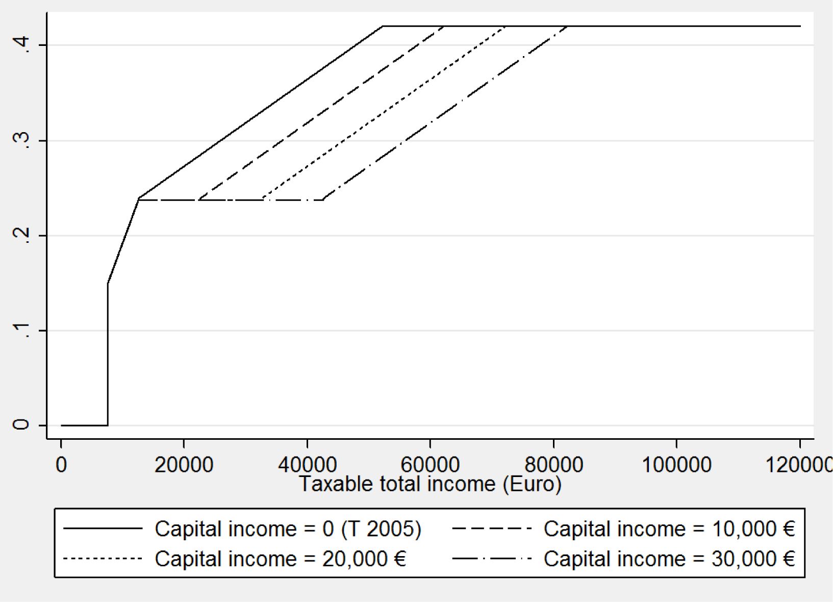
Marginal tax rates.
Source: Own calculations.
§ 32 a EStG-E defines the DIT income tax function: Let v denote taxable income in Euro (rounded down to the next Euro) according to § 2 Section 5 Clause 1 EStG-E, and let K denote capital income in the sense of § 2 Section 3 Clause 2 EStG-E (also rounded down to the next Euro). Then the personal income tax T amounts to
| T = 0 | if v ≤ 7664 |
| T = 883.74x2 + 1500x | if 7665 ≤ v ≤ 12584 |
| if 12585 ≤ v ≤ 12585 + K | |
| if 12586 + K ≤ v ≤ 12739 + K | |
| if 12740 + K ≤ v ≤ 52151 + K | |
| if v ≥ 52152 + K |
where
| x | = | ( v-7664)/10000 |
| y | = | ( v-7664-K )/10000 |
| z | = | ( v-12739-K )/10000 |
(x, y, z are also rounded down to the next Euro). The symbol t denotes the solidarity surcharge (i.e. currently t = 0.055).
Figure 1 shows marginal tax rates, i.e. the tax rates that apply to the last Euro of the tax base. It compares the current marginal tax schedule (based on § 32 a EStG) with the DIT schedule for taxpayers with fixed taxable capital incomes of different amounts. The solid line shows the current tax rates (T 2005). Under a dual tax regime this line refers to taxpayers without any capital income. For taxpayers with capital income a so-called stretched tax scale is applied. This means that the taxation of capital income is incorporated in the tax schedule in terms of a proportional zone. The length of this variable proportional band depends on the amount of taxable capital income. The return component of income is taxed proportionally while any profits beyond those are taxed progressively as labor income. As examples, I use marginal tax rates for capital incomes of 10,000, 20,000 and 30,000 Euro.
3. Labour supply of single persons
To quantify the labor supply incentives of a DIT introduction, I use a discrete choice structural labor supply model. The basic idea is to replace the budget set of a household with a finite number of points, and optimize over this set of points. I first set out the theory, estimation and simulation results for single persons. In the following section, I turn to persons living in couples.
3.1 Theory
I represent any individual’s choice set by a six-state labor supply regime and approximate actual hours per week ha by hours levels h ∈ H := {0,10,20,30,40,50} applying the following rounding rule
For all elements h in the choice set H I use GMOD to calculate household net incomes as
where w denotes the gross wage rate, μ is income from sources other than employment and T(·) is the tax-benefit function conditional on a vector of observed characteristics x. I assume that preferences can be represented by a utility function U and that individuals act as if to maximize utility
subject to the budget constraint
where denotes total time endowment.
To obtain random utilities (needed for estimation and simulation), I add state-specific random errors e(h) to utilities for all states h ∈ H. This gives random utilities
If the state-specific random errors are i.i.d. Type I extreme value distributed, then the probability P of working hj hours is
For the specification of the utility function, I follow the tradition started by Keane and Moffit (1998) and choose a flexible form quadratic direct utility function. Written in terms of individual consumption c = c(h) and leisure I obtain
where αcc, αll, αcl, βc and βl denote unknown parameters. I assume that preferences vary through taste-shifters on income and leisure coefficients:
where γc0, gc, γl0 and gl denote unknown coefficients and x is a (row) vector of individual characteristics2 and following van Soest (1995) dummy variables for part-time categories in order to capture the disutility of inflexible arrangements in the utility functions.
I deal with unobserved wage rates by estimating the expected market wage rates conditional on observed characteristics using Heckman’s two-step approach: I first estimate a reduced form participation equation, get the Mill’s rate and use it in a Mincer-type wage equation to correct for sample selection bias. I account for wage rate prediction errors by integrating out the disturbance term of the wage equation in the likelihood as suggested by van Soest (1995).
Estimation of the unknown preference parameters is based on a mixed logit model proposed by McFadden and Train (2000). Under mild regularity conditions, it can approximate the choice probabilities of any discrete choice model derived from random utility maximization as closely as desired. Under the assumption that the income coefficients are normally distributed and all other coefficients are fixed I proceed by maximum simulated likelihood.
3.1.1 Simulation
I use the parameters of the estimated utility functions to simulate the effects of the introduction of a Dual Income Tax on labor supply following the individual calibration procedure described by Kreedy and Kalb (2005, page 720 et seq.) Based on the selected sample I use hours worked to obtain a starting point for simulation.
For each individual, unobserved utility components (error terms) are drawn from the type I extreme value distribution and added to the measured utility in each of the hours points. A draw is accepted, if it results in the observed labor supply being the optimal choice for the individual. Otherwise, the draw is rejected, and another error term is drawn and checked. This is repeated until all sets of error terms are drawn and accepted. For each individual in the sample, this exercise is repeated 100 times.
The resulting sets of error terms drawn are possible values leading to the observed hours worked. Given individual characteristics and the draws, I can determine post-reform utility at each hours point. This generates a distribution of post-reform hours worked, conditional on the observed pre-reform hours, for each individual. The results of the draws can be summarized in transition tables.
3.2 Empirical results
3.2.1 Sample selection
The starting point for my sample is the base data file described above. First, I concentrate on single adult respondents. I exclude persons younger than 25 or older than 55 years of age, persons in education, pensioners, persons doing compulsory community or military services, persons receiving profit incomes only and civil servants. After dropping persons with missing observations of crucial variables, I receive a sample with 1,116 single men and another sample with 1,312 single women.
3.2.2 Estimation
The main preference parameter estimates for single men and single women are given in Table 4 in the Appendix. The estimated parameter values are consistent with economic theory. The marginal utility of net income and of leisure are statistically significant at least at the five percent level, they are positive and declining with income. The interaction effect between leisure and income is practically zero. Not surprisingly, there is less desire to work if an individual is handicapped, or if there is a nursing case in the family. For single mothers, there is less desire to work, the effect being smaller for older children. The main difference between male and female preferences is the role of children: While the number of children in different age groups has the expected sign and magnitude for women, these variables were not significant for men and so were dropped.
In Table 4 I do not report the estimates of the part-time dummies for part-time choice opportunities. For men and women, they all are negative and highly significant. This reflects the fact that low demand for part-time workers requires more effort (and hence less utility) to find part-time employment. Furthermore, all estimated standard errors of the random coefficients were highly significant. This suggests considerable unobserved heterogeneity of preferences. The traditional conditional logit approach is strongly rejected!
3.2.3 Simulation
Tables 1 and 2 present the simulation results for the labor supply of single persons. The last column gives the distribution of labor supply before the reform, the last row refers to the distribution after the reform. The numbers inside the matrix are row percentages indicating the probability of individuals from one hours point to another one.3
Labor supply transition matrix for single men.
| Post-reform hours | |||||||
|---|---|---|---|---|---|---|---|
| Pre-reform hours | 0 | 10 | 20 | 30 | 40 | 50 | % (row) |
| 0 | 16.55 | 0.00 | 0.01 | 0.26 | 0.56 | 0.20 | 17.59 |
| 10 | 0.00 | 2.12 | 0.00 | 0.04 | 0.05 | 0.08 | 2.29 |
| 20 | 0.00 | 0.00 | 1.79 | 0.01 | 0.02 | 0.04 | 1.85 |
| 30 | 0.00 | 0.00 | 0.00 | 17.43 | 0.20 | 0.13 | 17.77 |
| 40 | 0.01 | 0.00 | 0.00 | 0.01 | 42.05 | 0.24 | 42.30 |
| 50 | 0.00 | 0.00 | 0.00 | 0.00 | 0.03 | 18.18 | 18.21 |
| % (column) | 16.56 | 2.12 | 1.79 | 17.75 | 42.91 | 18.87 | 100.00 |
-
Source: Own calculations. Any summing errors are due to rounding.
Labor supply transition matrix for single women.
| Post-reform hours | |||||||
|---|---|---|---|---|---|---|---|
| Pre-reform hours | 0 | 10 | 20 | 30 | 40 | 50 | % (row) |
| 0 | 17.54 | 0.07 | 1.27 | 3.32 | 2.78 | 0.21 | 25.19 |
| 10 | 0.04 | 4.02 | 0.18 | 0.66 | 0.53 | 0.08 | 5.51 |
| 20 | 0.04 | 0.02 | 8.49 | 0.46 | 0.42 | 0.08 | 9.50 |
| 30 | 0.17 | 0.00 | 0.02 | 20.72 | 0.30 | 0.05 | 21.27 |
| 40 | 0.17 | 0.02 | 0.03 | 0.05 | 31.77 | 0.02 | 32.05 |
| 50 | 0.14 | 0.01 | 0.10 | 0.09 | 0.08 | 6.07 | 6.49 |
| % (column) | 18.11 | 4.13 | 10.09 | 25.29 | 35.88 | 6.50 | 100.00 |
-
Source: Own calculations. Any summing errors are due to rounding.
My results suggest that – in a short run partial equilibrium view – the DIT reform suggested by the German Council of Economic Experts (2008) will generate only small labor supply reactions. For single persons, on average, they will be slightly positive.
4. Labor supply of couples
4.1 Theory
For married or cohabiting couples I allow for joint decision making. Each partner may account for the decision of the other partner when deciding on hours worked. I assume that each household member selects one of six regimes: non-participation or one of five employment states ℏ ∊ H = {0,10,20,30,40,50} (the elements denoting hours per week). Thus, the choice set for couples is H × H. Actual individual working hours observed in the data are rounded (as above) to fit the elements in this set.
I assume that preferences of a couple may be represented by a flexible quadratic utility function
Here denotes leisure and h hours worked of male ( m ) or female ( f ) persons, while c denotes their joint net income. The α and β coefficients are unknown population parameters. The sign of αfm indicates whether male and female leisure are substitutes or complements. Similar to the case of single persons, some preference parameters depend on personal, household and other characteristics. Supplementing representative household utility I add stochastic terms accounting for state specific errors (needed for estimation and simulation) and finally derive the probability of choosing any consumption-leisure combination in the set of feasible household decisions. Estimation proceeds via mixed logit and simulation by calibration4 as described above. I derive household gross earnings assuming state invariant male and female gross wage rates, and calculate the corresponding state specific net household income for each hours combination in the choice set H × H using GMOD and my base data set described above.
4.2 Empirical results
4.2.1 Sample Selection
Starting point for my analysis is again the base data file described above, now concentrating on couples. I apply the sample selection criteria as described for singles to both partners and obtain a sample of 2,015 couples.
4.2.2 Estimation
The main preference parameter estimates for married and cohabiting couples are given in Table 5 in the Appendix. The estimated parameter values are consistent with economic theory. The marginal utility of both partners’ leisures and the marginal utility of net income are highly significant, positive and declining with income. The interaction effect between male and female leisure is statistically not different from zero and practically unimportant. Not surprisingly, there is less desire to work for mothers, the effect being smaller for older children.
Due to space restrictions, in Table 6 I do not report the estimates of the part-time dummies for part-time choice opportunities. (But they are used in the simulation exercises.) For both sexes, they all are negative and highly significant. As in the case of singles, this reflects the fact that low demand for part-time workers requires more effort to find part-time employment. Again, all estimated standard errors of the random coefficients were highly significant. As for singles, this suggests considerable unobserved heterogeneity of preferences of couples. Again, the traditional conditional logit approach is strongly rejected!
4.2.3 Simulation
Tables 3 and 4 show that the partial equilibrium impact of the reform proposal on the labor supply of couples is relatively small. As was to be expected, positive incentive effects are most likely for married females. This result, not shown in an extra table, is in line with the vast majority of previous studies on female labor supply.
Labor supply transition matrix for men in couples.
| Post-reform hours | |||||||
|---|---|---|---|---|---|---|---|
| Pre-reform hours | 0 | 10 | 20 | 30 | 40 | 50 | % (row) |
| 0 | 9.41 | 0.00 | 0.01 | 0.03 | 0.08 | 0.06 | 9.59 |
| 10 | 0.00 | 0.48 | 0.00 | 0.00 | 0.00 | 0.00 | 0.49 |
| 20 | 0.00 | 0.00 | 1.00 | 0.00 | 0.01 | 0.00 | 1.02 |
| 30 | 0.03 | 0.00 | 0.00 | 16.38 | 0.10 | 0.10 | 16.61 |
| 40 | 0.08 | 0.00 | 0.02 | 0.12 | 50.31 | 0.13 | 50.66 |
| 50 | 0.04 | 0.00 | 0.01 | 0.05 | 0.18 | 21.35 | 21.62 |
| % (column) | 9.55 | 0.49 | 1.05 | 16.58 | 50.68 | 21.65 | 100.00 |
-
Source: Own calculations. Any summing errors are due to rounding.
Labor supply transition matrix for women in couples.
| Post-reform hours | |||||||
|---|---|---|---|---|---|---|---|
| Pre-reform hours | 0 | 10 | 20 | 30 | 40 | 50 | % (row) |
| 0 | 33.78 | 0.14 | 0.26 | 0.19 | 0.24 | 0.02 | 34.63 |
| 10 | 0.02 | 10.88 | 0.05 | 0.07 | 0.02 | 0.00 | 11.05 |
| 20 | 0.01 | 0.00 | 15.71 | 0.02 | 0.06 | 0.00 | 15.82 |
| 30 | 0.01 | 0.02 | 0.03 | 16.63 | 0.07 | 0.04 | 16.81 |
| 40 | 0.00 | 0.00 | 0.01 | 0.02 | 17.96 | 0.04 | 18.04 |
| 50 | 0.00 | 0.00 | 0.01 | 0.01 | 0.01 | 3.62 | 3.66 |
| % (column) | 33.83 | 11.05 | 16.07 | 16.95 | 18.37 | 3.73 | 100.00 |
-
Source: Own calculations. Any summing errors are due to rounding.
5. Aggregate results
If I finally aggregate my results over persons living as singles and living in couples, I find a positive incentive effect of the introduction of a DIT. On average, labor supply increases. But does working time increase as well?
If you accept my results and the German Council of Economic Experts assumption of a 1.1 percent reform-induced increase in labor demand, then in the whole economy annual working time will increase on average and in the aggregate. This effect, combined with the smaller tax burden on capital income, yields an increase in aggregate net income. Thus, a DIT induced demand-side driven growth – as suggested by CGE studies – is indeed possible.
6. Conclusion
This paper evaluates the incentive effects of a Dual Income Tax reform in Germany based on GMOD, a tax-benefit microsimulation model, and on a sample of thousands of households representative for the German population. Instead of invoking the assumption of one given labor supply elasticity as current general equilibrium simulation models do, I allow for labor supply responses of the persons in a sample representative for the resident population in Germany. I do not present estimated elasticities, but my results are based on estimated responses of individuals in a representative sample. Estimates are obtained with a highly flexible mixed logit simulation approach. It includes the traditional conditional logit model used in a former study as a special case (which is rejected).
The main finding is that reform induced labor supply responses are small, but – on average – positive. Thus, my results empirically support the central, but untested, labor supply assumptions in traditional CGE models.
Further research is needed to assess the detailed impact of a DIT in Germany on the distribution of income and of individual economic welfare. This promises additional advantages in policy advising in comparison to computable equilibrium simulation models and may be a useful supplementation to these approaches.
Footnotes
1.
A more comprehensive version of this report, available only in German, includes an elaborate tax amending bill of the income tax law proposed (EStG-E). (See Sachverständigenrat zur Begutachtung der gesamtwirtschaftlichen Entwicklung, Max- Planck-Institut für Geistiges Eigentum, Wettbewerbs- Und Steuerrecht, Zentrum für Europäische Wirtschaftsforschung, 2006).
2.
Individual characteristics embedded are age and age squared, place of residence in East Germany (yes=1, no=0), nursing case in the family (yes=1, no=0), citizenship (not German = 1, German=0), high education, i.e. degree from universities or from universities of applied sciences (yes=1, no=0), low education, i.e. no vocational qualification attained (yes=1, no=0), handicapped person (yes=1, no=0), number of children under 6, and number of children between 6 and 16.
3.
See Kreedy and Kalb (2005) for a very detailed explanation of labor supply transition matrices.
4.
“Individual” calibration now refers to calibration based on the estimated preference functions of the couples.
Appendix 1
Estimated preference parameters, singles.
| Single Men | Single Women | |
| Income | 0.0680 | 0.183** |
| (0.0363) | (0.0630) | |
| Income2 | −0.000264 | −0.00291* |
| (0.000403) | (0.00121) | |
| Leisure | 0.371*** | 0.842*** |
| (0.0806) | (0.123) | |
| Leisure2 | −0.00287 *** | −0.00469 *** |
| (0.000399) | (0.000496) | |
| Leisure*income | −0.00128 | −0.00233** |
| (0.000653) | (0.000779) | |
| Leisure*age | −0.00425 | −0.0159** |
| (0.00361) | (0.00536) | |
| Leisure*age2 | 0.0000545 | 0.000205** |
| (0.0000464) | (0.0000682) | |
| Leisure*(East Germany?) | 0.0218* | −0.00203 |
| (0.00872) | (0.00982) | |
| Leisure*(Nursing case in family?) | 0.0126 | −0.00950 |
| (0.0240) | (0.0215) | |
| Leisure*foreign? | 0.0297** | −0.0209 |
| (0.0112) | (0.0190) | |
| Leisure*(high education?) | −0.0355** | −0.0289** |
| (0.0113) | (0.0104) | |
| Leisure*(low education?) | 0.0229** | 0.0300* |
| (0.00848) | (0.0147) | |
| Leisure*handicapped? | 0.0363** | 0.00161 |
| (0.0133) | (0.0226) | |
| Leisure*(no. of kids under 6) | 0.0700 *** | |
| (0.0122) | ||
| Leisure*(no. of kids age 6-16) | 0.0358 *** | |
| (0.00662) | ||
| Standard Deviation | ||
| Income | 0.0902 *** | 0.154*** |
| (0.0225) | (0.0307) | |
| Observations | 1116 | 1312 |
| Standard errors in parentheses | ||
-
*
p < 0.05.
-
**
p < 0.01.
-
*
p < 0.001.
A description of the sample for 1997, 1998, and 1999.
| Coefficient | Std. Err. | |
|---|---|---|
| Income | 0.0644** | (0.0197) |
| Income2 | 0.0004954 | (0.0000644) |
| Female’s leisure | 0.486*** | (0.108) |
| (Female’s leisure) | −0.00364 *** | (0.000661) |
| Male’s leisure | 0.268* | (0.107) |
| (Male’s leisure) | −0.00319 *** | (0.000315) |
| (Female’s leisure)*(male’s leisure) | −0.000448 | (0.000282) |
| (Female’s leisure)*(female’s*age) | −0.00333 | (0.00360) |
| (Female’s leisure)*(female’s*age)2 | 0.0000542 | (0.0000450) |
| (Female’s leisure)*(East Germany?) | −0.0434*** | (0.00763) |
| (Female’s leisure)*(no. of kids under 6) | 0.0701*** | (0.0101) |
| (Female’s leisure)*(no. of kids aged 616) | 0.0301 *** | (0.00492) |
| (Female’s leisure)*(nursing case in family?) | 0.0346 | (0.0181) |
| (Female’s leisure)*(married?) | 0.0320** | (0.0108) |
| (Male’s leisure)*(male’s*age) | 0.00514 | (0.00470) |
| (Male’s leisure)*(male’s*age)2 | −0.0000484 | (0.0000555) |
| (Male’s leisure)*(East Germany?) | 0.00857 | (0.00881) |
| (Male’s leisure)*(no. of kids under 6) | 0.00257 | (0.00715) |
| (Male’s leisure)*(no. of kids aged 6-16) | 0.000312 | (0.00439) |
| (Male’s leisure)*(nursing case in family?) | 0.0181 | (0.0126) |
| (Male’s leisure)*(married?) | −0.0158 | (0.0110) |
| Standard Deviation | ||
| Income | 0.0745** | |
| (0.0233) | ||
| Sample Size | 2015 | |
| Log-likelihood | −14161577 | |
-
*
p < 0.05.
-
**
p < 0.01.
-
***
p < 0.001.
-
Note: A question mark means that the variable is binary, coded 1 for a “Yes” and 0 for a “No”.
References
-
1
MITAX - Mikroanalysen und Steuerpolitik54–83, Steuerreformplane im empirischen Vergleich, MITAX - Mikroanalysen und Steuerpolitik, Statistik und Wissenschaft, Band 7, Wiesbaden, Statistisches Bundesamt. Beitrage zur wissenschaftlichen Konferenz am 6. und 7. Oktober 2005 in Lüneburg.
-
2
Discrete hours labour supply modelling: Specification, estimation and simulationJournal of Economic Surveys 19:697–734.
-
3
Moving towards Dual Income Taxation in EuropeFinanzArchiv: Public Finance Analysis 63:436–456.
-
4
Dual Income Tax. A Proposal for Reforming Corporate and Personal Income Tax in GermanyHeidelberg: Physica-Verlag.
-
5
Reformoption Duale Einkommensteuer - Aufkommens- und Verteilungseffekte. IAW-Diskussionspapier 58Tübingen: Institut für Angewandte Wirtschaftsforschung.
-
6
A structural model of multiple welfare program participation and labor supplyInternational Economic Review 39:553–589.
- 7
- 8
-
9
Capital income taxation and the Dual Income Tax. Technical report, Policy Research Institute, Ministry of Finance of Japan. PRI Discussion Paper Series (No.04A-17)Capital income taxation and the Dual Income Tax. Technical report, Policy Research Institute, Ministry of Finance of Japan. PRI Discussion Paper Series (No.04A-17).
-
10
CGE Models and Capital Income Tax Reforms: The Case of a Dual Income Tax for GermanyLecture Notes in Economics and Mathematical Systems, Vol. 601, Springer, Berlin-Heidelberg.
-
11
Reform der Einkommens- und Unternehmensbesteuerung durch die Duale EinkommensteuerReform der Einkommens- und Unternehmensbesteuerung durch die Duale Einkommensteuer, Expertise im Auftrag der Bundesminister der Finanzen und für Wirtschaft und Arbeit vom 23. Februar 2005.
-
12
The Nordic Dual Income Tax: Principles, practices, and relevance for CanadaCanadian Tax Journal 55:557–602.
-
13
Structural models of family labor supply: A discrete choice approachJournal of Human Resources 30:63–88.
-
14
Implementing a Dual Income Tax in Germany. Effects on labor supply and income distributionJournal of Economics and Statistics 229:84–102.
Article and author information
Author details
Acknowledgements
The data used in this publication were made available by the German Socio-Economic Panel Study (GSOEP) at the German Institute for Economic Research (DIW), Berlin.
The author is greatly indebted to Gijs Dekkers, Ulrich Scheurle and two anonymous referees for valuable comments.
Publication history
- Version of Record published: August 31, 2011 (version 1)
Copyright
© 2011, Wagenhals
This article is distributed under the terms of the Creative Commons Attribution License, which permits unrestricted use and redistribution provided that the original author and source are credited.