Dual income tax reform in Germany: A microsimulation approach
- Universität Hohenheim, Germany
Cite this article
as: G. Wagenhals; 2011; Dual income tax reform in Germany: A microsimulation approach; International Journal of Microsimulation; 4(2); 3-13.
doi: 10.34196/ijm.00049
- Article
- Figures and data
- Jump to
Figures
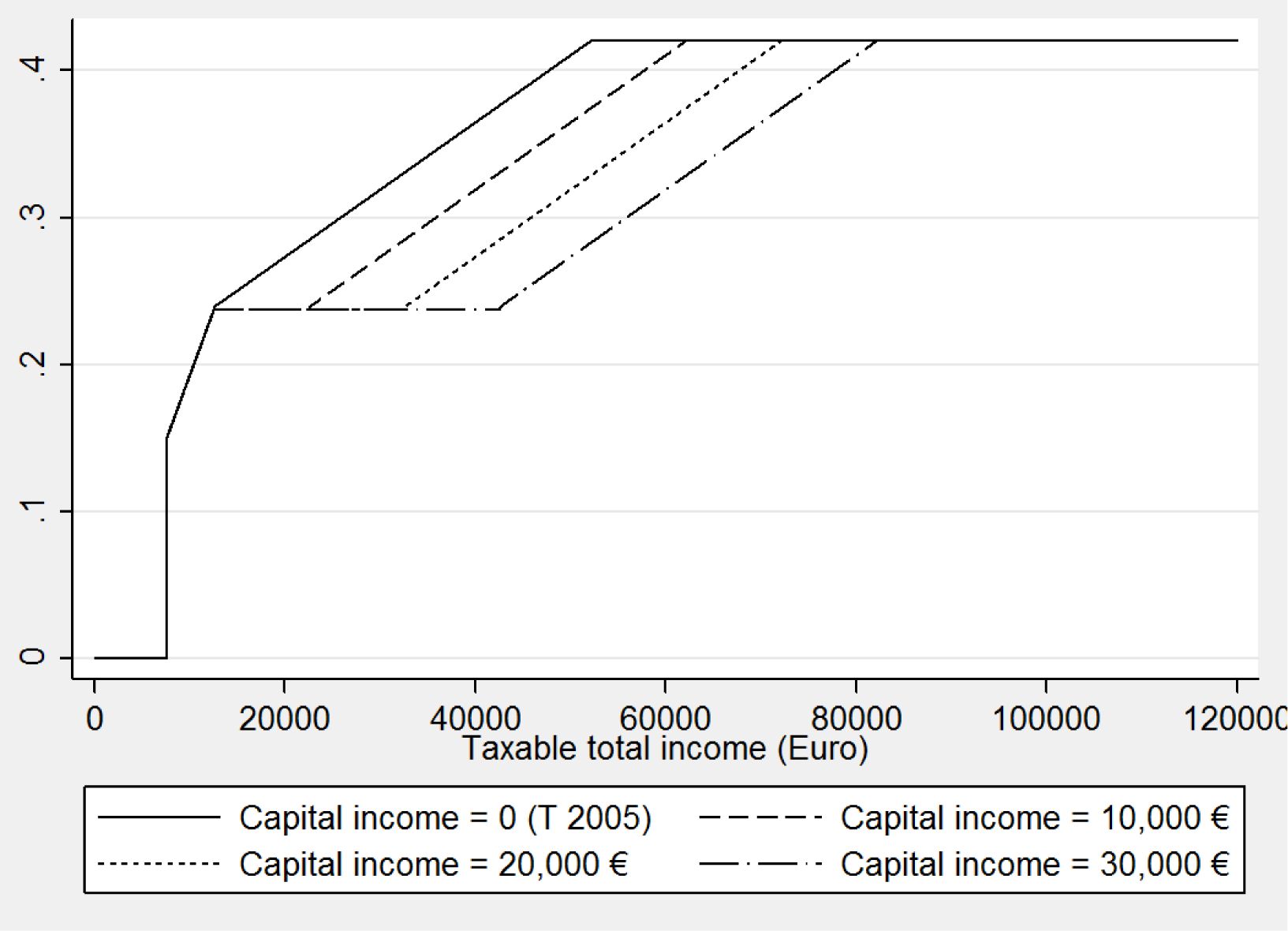
Figure 1

Marginal tax rates.
Source: Own calculations.
Tables
Table 1
Labor supply transition matrix for single men.
| Post-reform hours | |||||||
|---|---|---|---|---|---|---|---|
| Pre-reform hours | 0 | 10 | 20 | 30 | 40 | 50 | % (row) |
| 0 | 16.55 | 0.00 | 0.01 | 0.26 | 0.56 | 0.20 | 17.59 |
| 10 | 0.00 | 2.12 | 0.00 | 0.04 | 0.05 | 0.08 | 2.29 |
| 20 | 0.00 | 0.00 | 1.79 | 0.01 | 0.02 | 0.04 | 1.85 |
| 30 | 0.00 | 0.00 | 0.00 | 17.43 | 0.20 | 0.13 | 17.77 |
| 40 | 0.01 | 0.00 | 0.00 | 0.01 | 42.05 | 0.24 | 42.30 |
| 50 | 0.00 | 0.00 | 0.00 | 0.00 | 0.03 | 18.18 | 18.21 |
| % (column) | 16.56 | 2.12 | 1.79 | 17.75 | 42.91 | 18.87 | 100.00 |
-
Source: Own calculations. Any summing errors are due to rounding.
Table 2
Labor supply transition matrix for single women.
| Post-reform hours | |||||||
|---|---|---|---|---|---|---|---|
| Pre-reform hours | 0 | 10 | 20 | 30 | 40 | 50 | % (row) |
| 0 | 17.54 | 0.07 | 1.27 | 3.32 | 2.78 | 0.21 | 25.19 |
| 10 | 0.04 | 4.02 | 0.18 | 0.66 | 0.53 | 0.08 | 5.51 |
| 20 | 0.04 | 0.02 | 8.49 | 0.46 | 0.42 | 0.08 | 9.50 |
| 30 | 0.17 | 0.00 | 0.02 | 20.72 | 0.30 | 0.05 | 21.27 |
| 40 | 0.17 | 0.02 | 0.03 | 0.05 | 31.77 | 0.02 | 32.05 |
| 50 | 0.14 | 0.01 | 0.10 | 0.09 | 0.08 | 6.07 | 6.49 |
| % (column) | 18.11 | 4.13 | 10.09 | 25.29 | 35.88 | 6.50 | 100.00 |
-
Source: Own calculations. Any summing errors are due to rounding.
Table 3
Labor supply transition matrix for men in couples.
| Post-reform hours | |||||||
|---|---|---|---|---|---|---|---|
| Pre-reform hours | 0 | 10 | 20 | 30 | 40 | 50 | % (row) |
| 0 | 9.41 | 0.00 | 0.01 | 0.03 | 0.08 | 0.06 | 9.59 |
| 10 | 0.00 | 0.48 | 0.00 | 0.00 | 0.00 | 0.00 | 0.49 |
| 20 | 0.00 | 0.00 | 1.00 | 0.00 | 0.01 | 0.00 | 1.02 |
| 30 | 0.03 | 0.00 | 0.00 | 16.38 | 0.10 | 0.10 | 16.61 |
| 40 | 0.08 | 0.00 | 0.02 | 0.12 | 50.31 | 0.13 | 50.66 |
| 50 | 0.04 | 0.00 | 0.01 | 0.05 | 0.18 | 21.35 | 21.62 |
| % (column) | 9.55 | 0.49 | 1.05 | 16.58 | 50.68 | 21.65 | 100.00 |
-
Source: Own calculations. Any summing errors are due to rounding.
Table 4
Labor supply transition matrix for women in couples.
| Post-reform hours | |||||||
|---|---|---|---|---|---|---|---|
| Pre-reform hours | 0 | 10 | 20 | 30 | 40 | 50 | % (row) |
| 0 | 33.78 | 0.14 | 0.26 | 0.19 | 0.24 | 0.02 | 34.63 |
| 10 | 0.02 | 10.88 | 0.05 | 0.07 | 0.02 | 0.00 | 11.05 |
| 20 | 0.01 | 0.00 | 15.71 | 0.02 | 0.06 | 0.00 | 15.82 |
| 30 | 0.01 | 0.02 | 0.03 | 16.63 | 0.07 | 0.04 | 16.81 |
| 40 | 0.00 | 0.00 | 0.01 | 0.02 | 17.96 | 0.04 | 18.04 |
| 50 | 0.00 | 0.00 | 0.01 | 0.01 | 0.01 | 3.62 | 3.66 |
| % (column) | 33.83 | 11.05 | 16.07 | 16.95 | 18.37 | 3.73 | 100.00 |
-
Source: Own calculations. Any summing errors are due to rounding.
Table 5
Estimated preference parameters, singles.
| Single Men | Single Women | |
| Income | 0.0680 | 0.183** |
| (0.0363) | (0.0630) | |
| Income2 | −0.000264 | −0.00291* |
| (0.000403) | (0.00121) | |
| Leisure | 0.371*** | 0.842*** |
| (0.0806) | (0.123) | |
| Leisure2 | −0.00287 *** | −0.00469 *** |
| (0.000399) | (0.000496) | |
| Leisure*income | −0.00128 | −0.00233** |
| (0.000653) | (0.000779) | |
| Leisure*age | −0.00425 | −0.0159** |
| (0.00361) | (0.00536) | |
| Leisure*age2 | 0.0000545 | 0.000205** |
| (0.0000464) | (0.0000682) | |
| Leisure*(East Germany?) | 0.0218* | −0.00203 |
| (0.00872) | (0.00982) | |
| Leisure*(Nursing case in family?) | 0.0126 | −0.00950 |
| (0.0240) | (0.0215) | |
| Leisure*foreign? | 0.0297** | −0.0209 |
| (0.0112) | (0.0190) | |
| Leisure*(high education?) | −0.0355** | −0.0289** |
| (0.0113) | (0.0104) | |
| Leisure*(low education?) | 0.0229** | 0.0300* |
| (0.00848) | (0.0147) | |
| Leisure*handicapped? | 0.0363** | 0.00161 |
| (0.0133) | (0.0226) | |
| Leisure*(no. of kids under 6) | 0.0700 *** | |
| (0.0122) | ||
| Leisure*(no. of kids age 6-16) | 0.0358 *** | |
| (0.00662) | ||
| Standard Deviation | ||
| Income | 0.0902 *** | 0.154*** |
| (0.0225) | (0.0307) | |
| Observations | 1116 | 1312 |
| Standard errors in parentheses | ||
-
*
p < 0.05.
-
**
p < 0.01.
-
*
p < 0.001.
Table 6
A description of the sample for 1997, 1998, and 1999.
| Coefficient | Std. Err. | |
|---|---|---|
| Income | 0.0644** | (0.0197) |
| Income2 | 0.0004954 | (0.0000644) |
| Female’s leisure | 0.486*** | (0.108) |
| (Female’s leisure) | −0.00364 *** | (0.000661) |
| Male’s leisure | 0.268* | (0.107) |
| (Male’s leisure) | −0.00319 *** | (0.000315) |
| (Female’s leisure)*(male’s leisure) | −0.000448 | (0.000282) |
| (Female’s leisure)*(female’s*age) | −0.00333 | (0.00360) |
| (Female’s leisure)*(female’s*age)2 | 0.0000542 | (0.0000450) |
| (Female’s leisure)*(East Germany?) | −0.0434*** | (0.00763) |
| (Female’s leisure)*(no. of kids under 6) | 0.0701*** | (0.0101) |
| (Female’s leisure)*(no. of kids aged 616) | 0.0301 *** | (0.00492) |
| (Female’s leisure)*(nursing case in family?) | 0.0346 | (0.0181) |
| (Female’s leisure)*(married?) | 0.0320** | (0.0108) |
| (Male’s leisure)*(male’s*age) | 0.00514 | (0.00470) |
| (Male’s leisure)*(male’s*age)2 | −0.0000484 | (0.0000555) |
| (Male’s leisure)*(East Germany?) | 0.00857 | (0.00881) |
| (Male’s leisure)*(no. of kids under 6) | 0.00257 | (0.00715) |
| (Male’s leisure)*(no. of kids aged 6-16) | 0.000312 | (0.00439) |
| (Male’s leisure)*(nursing case in family?) | 0.0181 | (0.0126) |
| (Male’s leisure)*(married?) | −0.0158 | (0.0110) |
| Standard Deviation | ||
| Income | 0.0745** | |
| (0.0233) | ||
| Sample Size | 2015 | |
| Log-likelihood | −14161577 | |
-
*
p < 0.05.
-
**
p < 0.01.
-
***
p < 0.001.
-
Note: A question mark means that the variable is binary, coded 1 for a “Yes” and 0 for a “No”.
Download links
A two-part list of links to download the article, or parts of the article, in various formats.