Microsimulation of indirect taxes
Abstract
The goal of this paper is to simulate a tax shift from labour to consumption and perform a distributional analysis of the reform. Microsimulation programs are often uniquely focussed on the personal income tax system and on social security contributions and benefits. However, against a political background where income taxes are under increased pressure and alternative, less distortive forms of taxation come under consideration, microsimulation models enriched with expenditure data and consumption tax structures could play an important role in sharpening the (distributional) picture of such systemic changes. The current paper discusses an algorithm for this enrichment – mainly with VAT, excises and other consumption taxes – within the context of the EUROMOD-framework and applies the obtained program to the simulation of a decrease of social security contributions compensated by a rise in standard VAT rate to maintain government budget neutrality for four EU countries. The measure is found to have a (first order) regressive effect, pointing to the fact that keeping redistribution constant would require the remaining post-reform income taxation to become more progressive.
1. Introduction
The current economic crisis and rising unemployment has put the plea for a reduction of the tax wedge on employment and an “alternative financing of the welfare state" again in the spotlight (see e.g. OECD, 2008). A major difficulty in the debate is that, although the arguments rest upon theoretical economic foundations1, little is known about the concrete consequences of policy proposals on the government budget and the redistribution level in society. Indeed, the lack of reliable predictions may be one of the reasons why so few of the reform proposals are eventually put into practice.
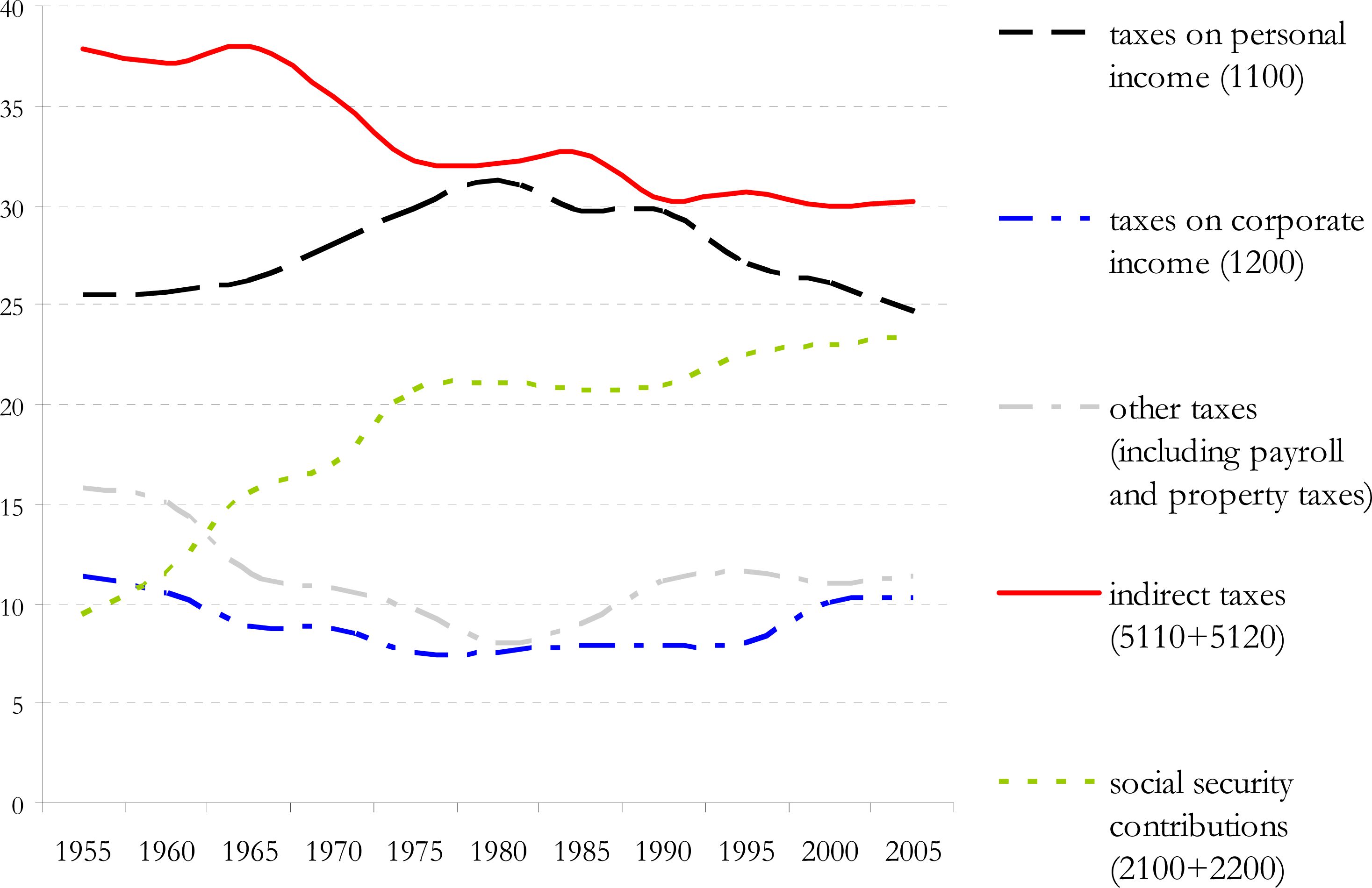
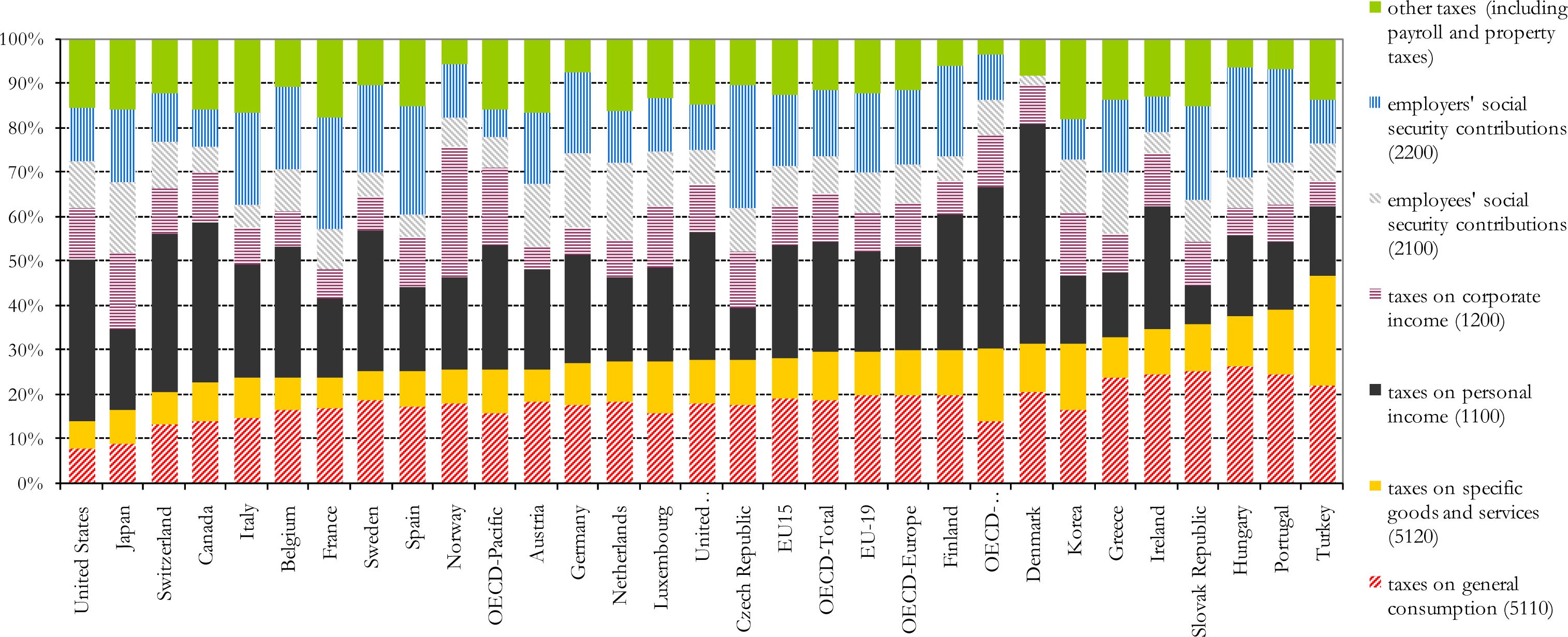
Since microsimulation models (MSM) are the tools par excellence for assessing the distributional impact of policy instruments, they form a good starting point in generating the desired predictions. Currently however, the prominent role of the consumption tax instrument both in practice (see Figure 1 and 2) and in the public debate, stands in sharp contrast with the poor attention it got within the microsimulation community. Indeed, most MSM'S have focussed on the arithmetic micromodelling of personal income taxes, social security contributions and benefits, not indirect taxes, despite the relative simplicity of most VAT and excise systems.
The basic reason for the omission of indirect taxes in standard MSM-modelling is of a practical nature: often the micro level income datasets used in tax benefit microsimulation do not contain information on expenditures which is detailed enough to calculate indirect tax liabilities with sufficient precision. To overcome this shortcoming (besides more comprehensive socio-economic surveys, in the long run), one could either design a separate indirect tax microsimulation model, running on e.g. a budget survey dataset, or impute expenditure information into the income dataset underlying an existing tax benefit model. In this paper, we adopted the second strategy for two reasons. Firstly, budget surveys in many countries do not contain enough detailed information to enable a microsimulation model like EUROMOD to run upon it. In most cases disposable income is available and sometimes a gross income measure. But, a disaggregation according to income source is seldom available in budget surveys. Secondly, the microsimulation model used here, EUROMOD2, makes standard use of European income datasets, the EU-SILC, because of the detail of income variables that it provides as well as the advantage of it offering standardized datasets across the countries of the European Union. EU-SILC, however, has no or only very limited expenditure information. Hence, the first objective of the paper is to suggest an algorithm for dealing with missing expenditure and consumption tax information in the context of a direct tax-and-benefit simulation context, like EUROMOD. In practice, we have been able to use budget surveys of four countries (Belgium, Hungary, Ireland and the UK) and implement our method for them.
The second objective of the paper is to simulate a concrete policy proposal involving a shift from labour to consumption tax, more specifically a 25% decrease of social security contributions combined with an offsetting increase in the standard VAT rate. While government budget neutrality is maintained, the analysis of the reform will focus on the distributional consequences. However, several caveats are in order in the interpretation of the results. First, the model is embedded in a partial equilibrium framework where producer prices are taken as exogenously given, which may be problematic since the price of labour changes3. Moreover, the routine contains only an (Engel-curve based) behavioural model for consumption, but not for labour supply. Since a shift of revenue collection from social security contributions towards indirect taxes is mostly intended to stimulate labour market participation and/or labour supply, which of course affects the income redistribution, the results presented here can only be taken as first-order effects. The incorporation of a labour supply model is an issue that will be addressed in future work.
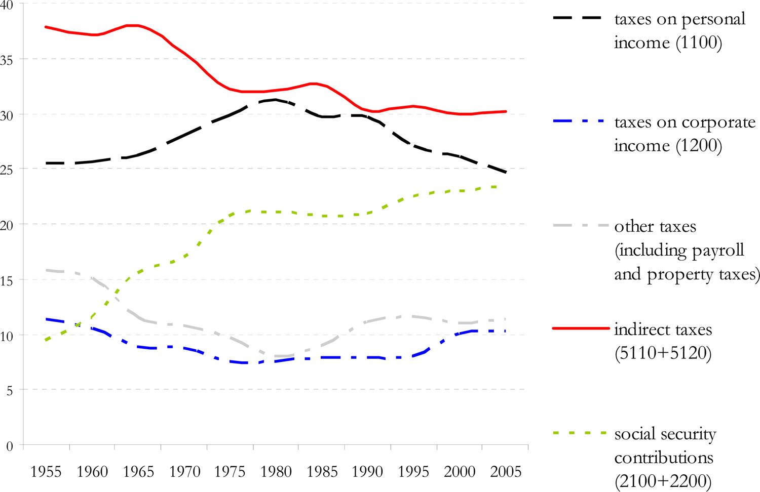
Share of different components of government revenue OECD 1955–2005.
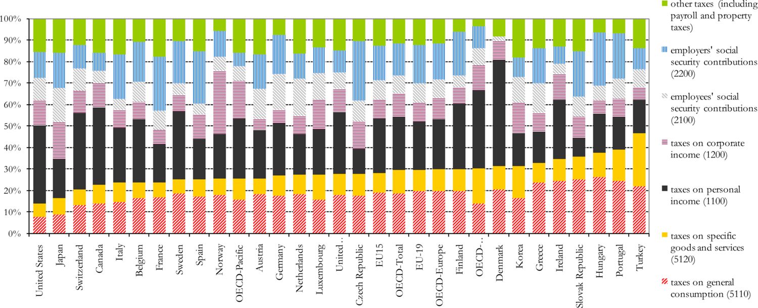
Share of different components of government revenue – oecd 2005.
The structure of the paper is as follows: in Section 2 we describe the data that are available and the implementation of the indirect tax system in the model. The imputation of expenditure data in the EUROMOD datasets is considered in Section 3. Finally, Section 4 contains the description and the results of the combined direct-indirect tax simulations.
2. Expenditure and tax data
The countries for which the imputation of expenditures into an income dataset took place are Belgium, Hungary, Ireland and the UK. These countries formed the subject of subproject 3 in the AIM-AP-project, the aim of which was to enrich EUROMOD with expenditure information and an indirect tax module. Table 1 summarizes the income and expenditure datasets used for each country.
Expenditure datasets and income datasets for the four countries.
| Country | budget survey | # of households | income survey | # of households | policy year indirect taxes |
|---|---|---|---|---|---|
| BE | Household Budget Survey 2003 | 3,550 | EU-SILC 2004 | 5,275 | 2003 |
| HU | Household Budget Survey 2005 | 8,710 | EU-SILC 2005 | 6,924 | 2005 |
| IE | Household Budget Survey 1999 | 7,644 | Living In Ireland 2000 | 3,644 | 2001 |
| UK | Family Expenditures Survey 2003/2004 | 7,048 | Family Resources Survey 2003/2004 | 28,768 | 2003 |
Typically, a euromod dataset contains sociodemographic background variables like age, sex, education level etc., as well as income and personal income tax variables. Euromod then subsequently performs a number of policy modules, which may be actual or reform policies, on the input variables to obtain the household disposable income.
Household budget surveys, on the other hand, consist of socio-demographic background variables, some of which overlap with those in the euromod datasets, and detailed expenditure information. To ensure comparability across these four countries, the same expenditure aggregation was used across the countries, close to the highest level of the coicop -scheme4. An indirect tax module was constructed, which calculated the average indirect tax rates for each coicop-aggregate, by aggregating the VAT, ad valorem taxes and excise paid at the most detailed level of the available budget surveys across all commodities belonging to a specific coicop-aggregate. This implicitly defined a VAT- and excise-rate for this specific coicop-aggregate, which was then applied to calculate indirect tax liabilities in the income surveys. More information on the calculation of these indirect tax liabilities for aggregate commodity groups can be found in Decoster et al. (2008). In the appendix we also present a flow chart with the different steps of imputation and simulation.
Table 2 summarizes the VAT-structure for the four countries. The indirect tax legislation of the year of the expenditure survey was used, except for Ireland. The main change in indirect tax legislation between the year of the survey and the current legislation (as of 2009) has occurred in Hungary, where the standard rate has been lowered from 25 to 20% and the reduced rate from 15 to 5%. This substantial change has to be kept in mind when interpreting the results. Also the temporary reduction of the VAT-rate from 17.5% to 15% in the UK as part of the macro-economic stimulus package, decided at the end of 2008, is not taken up.
The excise duties, which are levied as an amount per unit of quantity rather than as a percentage of the producer price, differ a lot across the four countries. The tax base for excise duties however, i.e. the commodities on which an excise tax is levied, are more or less the same across the different countries. In summary, the excise products are:mineraloilproducts(gasoline, (un)leaded petrol, …), alcoholic products (spirits, beer, wine, …) and tobacco products (cigarettes, cigars, …). The Ad Valorem excise tax mostly concerns tobacco products. In order to make the VAT and excise systems comparable, excise duties are here expressed as implied tax rates (meaning as a function of observed expenditures and quantities) rather than on a unit basis.
VAT-structure and expenditure shares per vat-category; excise rates and shares for the 3 most important excise good categories.
| Country and policy year | VAT | Excise | ||||||
|---|---|---|---|---|---|---|---|---|
| standar d rate 18–25% | not taxed or exempte d | reduced rate 1 4–6% | reduced rate 2 8–15% | Alcohol | Tobacco | Private transpor t | ||
| BE-2003 | Rates | 21 | 0 | 6 | 12 | 43.9 | 162.9 | 34.7 |
| Shares | 41.9 | 37.9 | 19.8 | 0.4 | 1.7 | 1.3 | 8.9 | |
| HU-2005 | Rates | 25 | 0 | 5 | 15 | 64.3 | 273.0 | 79.0 |
| Shares | 42.7 | 8.1 | 4.1 | 45.1 | 0.6 | 2.6 | 4.1 | |
| IE-2001 | Rates | 20 | 0 | - | 12.5 | 26.6 | 300.0 | 75.4 |
| Shares | 36.2 | 42.0 | - | 21.8 | 4.5 | 3.4 | 5.3 | |
| UK-2003 | Rates | 17.5 | 0 | 5 | - | 89.7 | 414.7 | 58.8 |
| shares | 57.7 | 36.3 | 6.1 | - | 1.9 | 2.2 | 8.0 | |
3. Imputation of expenditures
As stated earlier, we started from income datasets that are used in EUROMOD but contain no expenditure information. As far as the imputation of COICOP-expenditures in these income datasets is concerned, the relative performance of four different imputation methods was evaluated: using a distance function, grade correspondence, non parametric Engel curves and parametric Engel curves.5 A detailed account of this comparison is found in Decoster et al. (2007). The final choice, based both on theoretical, empirical and practical arguments of future implementation in MSM-models, was to use the parametric Engel curves (see e.g. Banks et al., 1997, for a thorough discussion). An Engel curve was estimated for each COICOP-aggregate on the expenditure dataset and used to predict values in the income dataset, using the specification:
where x is a measure of income or total expenditures (cf. infra) and O is a vector of household characteristics common to both datasets.
Three considerations are relevant in this context. Firstly, since the regressors used in the Engel curve have to be selected from variables that are common to both datasets, this puts a serious limitation on model specification. It also required a phase of thorough comparison and harmonization of these common variables. As an example, Figure 3 plots the quantiles of disposable income in the budget dataset as a function of the quantiles in the EUROMOD dataset for Belgium. Two conclusions can be drawn: first that there is a straight line component, pointing to equality of distributions, containing 98.7 % of the data; second, that there are divergences in the tails of the distributions. So for extremely low or high incomes, the matching procedure may not be very accurate.

QQ-plot for disposable income quantiles in budget dataset (dib) versus quantiles in income dataset (dii), Belgium (Euros per year).
Secondly, using disposable income in the estimation of expenditures per category was problematic for two reasons. Firstly, the income distributions in the expenditure dataset used for estimation and the income dataset on which we impute often differ, especially in the tails, as indicated above. If the latter distribution has fatter tails, the imputation has the character of an extrapolation and is hence much less stable. This leads to some undesirable imputation properties, such as a large proportion of negative expenditures in each category and a large proportion of very high expenditures for some consumption categories. In the latter case, the implied savings rate becomes extremely negative in the income dataset. Secondly, disposable income in the expenditure datasets can be negative or 0, though in practice only in about 0.1% of the cases. Reasons for this can be direct taxation, and in some countries loss or theft of stolen goods and loss of capital income. Note that this already makes the estimation of income shares very cumbersome. Moreover, it excludes the specification in terms of the logarithm of disposable income and its square, which is dominantly present in the literature.
To deal with these problems the imputation was split up in two steps. First, total expenditures and total durable expenditures were estimated upon disposable income and the common sociodemographic variables6. The (empiric) relation between disposable income and total expenditures is much smoother and hence more robust to problems of the kind described above. These two estimated equations were then used to predict total expenditures and total durable expenditures in the EUROMOD dataset (and to construct total nondurable expenditures by taking the difference between the two). In the second step, nondurable budget shares for each nondurable category were constructed as the share of the category in total nondurable expenditure. These shares were then estimated by the formula above (using total nondurable expenditures as x). The obtained equations (one for each category) were then used to impute shares in the income dataset. In this way, both total nondurable expenditures and nondurable expenditure shares per category were present in the income dataset. By multiplying these, the expenditures per category could be derived. A priori, it cannot be excluded that this method yields negative budget shares in the imputation. But since there are no observed negative values and because of the smoothening effect on extreme incomes in the first step, in practice it did not occur in this exercise. A program line was however included that would set the negative budget shares to zero and would standardize the shares to sum to one in case this would occur for other datasets.
A third remark concerns the replication of so called zero expenditures in the target dataset. Estimating a regression on a consumption aggregate like tobacco, which is not consumed by a majority of households, and then imputing tobacco expenditures, fails to reproduce a sufficient number of exact zeroes. For distributional analyses, this might produce a significant bias in the target dataset. The population was therefore divided into subgroups according to whether or not the households have expenditures on the different zero expenditure aggregates: smokers and non smokers, renters and home owners, users and non-users of public transport and users and non-users of education. Then it was assumed that all the 16 resulting subgroups have different preference structures. Hence, the Engel curves are estimated for each subgroup separately. To determine to which group a household in the income dataset belonged, a Tobit regression model was used for the group identification in the budget survey. For each zero expenditure variable, like smoking, an underlying propensity to smoke model was estimated in the budget survey. This model was then used to predict this probability for the observations in the income dataset. For each observation a random number was drawn from the inverse normal distribution function: if this number was smaller than the estimated probability, the observation was categorized as respectively a smoker, renter, etc. Finally the budget shares in the income dataset were predicted with the Engel curves for the right subgroup to complete the imputation procedure. When the subgroups were too small to estimate a model the technique of subgroup-referencing was used (see Decoster et al., 2009). This boils down to increasing the number of observations, and hence reducing the variation of the estimates, by adding observations of other subgroups. However, because of the different preference structures of thegroups, this introduces estimation bias. To reduce this bias a weighting scheme and dummy variables for the different subgroups are introduced.7
Table 3 gives a comparison between average observed expenditures per consumption aggregate in the budget survey and the average imputed value in the EUROMOD dataset, for the four countries. The results show that the imputation was fairly accurate, with some notable exceptions, e.g. the category food and non-alcoholic beverages in Ireland. This points to the fact that there is a large difference in the marginal distributions for some of the explanatory variables between the two datasets. For the particular case of Ireland, there was an overrepresentation of single-person, retired households in the budget survey (see Decoster et al., 2009), or an underrepresentation of these households in the EUROMOD dataset. Note that – in the absence of unaccounted interaction effects – this will not affect the conclusions presented here as long as the EUROMOD dataset is representative for the population. Home production is not included in the table.
Average expenditures per consumption category in budget and EUROMOD dataset.
| Commodity | expenditures in €, BE | expenditures in €, HU | expenditures in €, IE | expenditures in GBP, UK | ||||
|---|---|---|---|---|---|---|---|---|
| Budget Survey | EUROMOD | Budget Survey | EUROMOD | Budget Survey | EUROMOD | Budget Survey | EUROMOD | |
| food, non-alcoholic beverages | 4,183 | 4,050 | 1,813 | 1,675 | 4,620 | 8,215 | 2,617 | 2,121 |
| alcoholic beverages | 466 | 400 | 82 | 36 | 1,663 | 1,513 | 325 | 296 |
| tobacco | 275 | 279 | 191 | 170 | 644 | 1,098 | 280 | 321 |
| clothing and footwear | 1,395 | 1,284 | 442 | 380 | 1,848 | 1,493 | 1,183 | 916 |
| home fuels and electricity | 1,321 | 1,284 | 831 | 844 | 1,128 | 1,987 | 623 | 590 |
| rents | 1,418 | 1,560 | 59 | 62 | 681 | 913 | 691 | 543 |
| household services | 1,268 | 1,157 | 666 | 685 | 1,230 | 1,365 | 999 | 818 |
| health | 1,608 | 1,507 | 245 | 323 | 582 | 391 | 174 | 144 |
| private transport | 2,660 | 2,214 | 590 | 325 | 1,394 | 1,808 | 1,814 | 1,413 |
| public transport | 161 | 158 | 185 | 148 | 513 | 534 | 292 | 242 |
| communication | 803 | 758 | 460 | 437 | 739 | 1,223 | 551 | 457 |
| recreation and culture | 2,058 | 1,752 | 390 | 384 | 1,931 | 2,171 | 1,760 | 1,472 |
| education | 207 | 141 | 76 | 76 | 405 | 368 | 529 | 248 |
| restaurants and hotels | 2344 | 1,972 | 246 | 153 | 1,695 | 1,652 | 2,105 | 1,746 |
| other goods and services | 2,491 | 2,175 | 471 | 466 | 4,869 | 3,917 | 1,408 | 1,210 |
| Durables | 2,671 | 2,372 | 656 | 658 | 5,306 | 3,384 | 3,405 | 3,212 |
| All | 25,330 | 23,062 | 7,645 | 7,056 | 29,248 | 32,032 | 18,754 | 15,748 |
4. Simulations of direct and indirect taxation
Finally, matched income and expenditure data are used to simulate changes in indirect taxation and evaluate the distributional consequences of these changes for the four aforementioned countries. The social security contributions of the employees are decreased by 25%. Assuming government budget neutrality, the rise in the standard VAT rate necessary to compensate fully for this loss is calculated. Further assumptions are that the savings of the households are constant, as well as the amount of durable goods they purchase. Note that expenditure on durables can increase due to a rise in the VAT-rate. The households have the possibility to change their behaviour according to the Engel curves estimated in the imputation step. This means that only the direct effect of a rise in total nondurable expenditures on the budget shares of the aggregates is taken into account, not the cross price effects between the aggregates.
To evaluate the distributional implications of the tax reform, a measure of consumption based welfare gain was adopted, as explained in Capéau et al. (2008). A summary is given below.
Write the Marshallian demand functions as:
where x and q denote quantities and consumer prices8 respectively. In this case the expenditure function for the non durable commodities becomes:
U denoting the welfare level obtained from the preference representation function u (f(q, y)). This expenditure function is homogeneous of degree 0 in the level of non durable expenditures and consumer prices, allowing to transform each proportionate price change into a corresponding change of e. The function c(.) is the building block of the money metric welfare function (see King, 1983). E.g. for a household with non durable expenditures e0 and facing prices q0 welfare is measured as:
where qr is a set of reference prices to convert welfare U0 in the situation (q0, e0 ) into monetary units. Now use as reference prices the baseline prices q0. The welfare change due to the change in nominal non durable expenditures (from e0 to e1 ) and in consumer prices (from q0 to q1) is then calculated as follows:
where U1 ≡ u ( f (q1, e1 )) denotes the utility level in the post-reform situation and WG denotes the welfare gain.
The second term in the last equation equals e0. The first term in the right hand side of equation embodies the counterfactual situation of reaching the post-reform utility level at the pre-reform prices. This can be calculated by means of the Hicksian, or compensated demand functions, denoted here as:
leading to:
These compensated demands only take-up the real income effect, leaving relative prices unchanged. Hence they correspond to the quantities calculated as follows:
e* is therefore calculated as:
The welfare gain is then calculated as:
Note that this welfare gain can be decomposed into three different effects: one effect coming from the change in nominal non durable expenditures, an effect coming from the change in the aggregate price level of the nondurable consumer items, discarding the relative price change, and an effect coming from the change in the relative prices of the non durable consumer items. The decomposition is as follows:
The first term in the above expression is the change in nominal non durable expenditures. But this difference would be an overestimation of the welfare gain. The other two terms in squared brackets give the effect of the changing consumer prices. The first is the change in the general price level, discarding the relative price change. Concretely, it is an aggregate measure of price changes, namely the weighted average of the individual price changes, weighted by the quantities (to be interpreted as the Hicksian quantities, after adjusting the price level in a proportionate way). The inclusion of this term is intuitive:a rise in the general price level decreases the gain in welfare as measured by nominal expenditures alone, since one can purchase fewer quantities with the same money. The second term between square brackets, Δ2q, accounts then for the relative price effect, i.e. for the changing of the slope of the budget constraint. With our specific assumptions, , and hence the third price-change-term Δ2q vanishes. The term between square brackets then simplifies to:
and the welfare gain to
The last expression is very intuitive: to measure the welfare impact one looks at changes in quantities. These changes are evaluated at pre reform prices. The first expression allows for a decomposition of the welfare gain in an expenditure and a price effect. This decomposition will be used in the tables.
The results are summarized in the following three tables. Table 4 presents the changes in the government budget. The decrease of the social security contributions of the employees by 25% leads to a substantial necessary increase in the standard VAT-rate: 4 to 5 percentage points in Belgium, Ireland and the UK. But up to 9 percentage points for Hungary. It is clear that the rise in standard VAT rate is proportional to the relative importance of the social security contributions and the indirect tax system. Note that for Belgium, part of the government's loss is recuperated by an increase in taxable income and hence by a rise in personal income tax. The other countries do not exclude social security contributions from the taxable base and hence their PIT revenue stays the same.
Tables 5 and 6 show the welfare consequences for different subgroups of society. For each group and country, the average change in welfare WG is depicted, together with its two components: the change in nondurable expenditures and the price effect. The first component is everywhere positive, explained by the fact that disposable income can only increase by the tax reform and because savings are kept constant9.
The second component represents the price effect, which captures the rise in price levels. As no goods have their prices decreased, this effect is negative for every household. Taken together, one can see from Table 4 that the price effect dominates the change in expenditures in the lower equivalized expenditure deciles, so that the welfare effect of the reform is negative for those groups. For the higher deciles, the situation is reversed and these groups become better off after the reform.
This analysis of gainers and losers can be carried out for other subgroups of the population as well. The upper rows of Table 5 show the effects along the division poor – non poor, where poverty is defined as having equivalized expenditures lower than 60% of the median equivalized expenditures. As can be expected from the previous table, the reform is beneficiary to the group of non poor as a whole, but the group of poor is affected very badly. The same conclusion can be drawn for socio-economic divisions as in the lower part of the third table:people in more vulnerable positions, like the unemployed (except for Hungary, where they are almost unaffected), retired people and people receiving income support, lose by the reform, while employed workers gain by it.
Revenue effects of the simulation.
| BE | HU | IE | UK | |||||
|---|---|---|---|---|---|---|---|---|
| baseline | simulation | baseline | simulation | baseline | simulation | baseline | simulation | |
| SIC employee | 17,490 | -3,900 | 2,777 | -693 | 168,875 | -33,902 | 42,283 | -9,713 |
| PIT | 35,500 | + 1,763 | 4,608 | +0 | 1136,416 | +0 | 164,813 | +0 |
| Indirect tax | 14,400 | + 2,309 | 4,300 | + 731 | 443,139 | 34,791 | 71,717 | + 10,655 |
| VAT rate | 21% | 26% | 25% | 34% | 20% | 23.5% | 17.5% | 21.5% |
Decomposition of welfare change into total expenditure effect and price change – by decile.
| Decile equiv. non durable expend. | BE (EUR) | HU (EUR) | IR (EUR) | UK (EUR) | ||||||||
|---|---|---|---|---|---|---|---|---|---|---|---|---|
| Change nondur. exp. | Price effect | WG | Change nondur. exp. | Price effect | WG | Change nondur. Exp. | Price effect | WG | Change nondur. Exp. | Price effect | WG | |
| 1 | 43 | −193 | −150 | 22 | −70 | −47 | 0 | −59 | −58 | 9 | −50 | −42 |
| 2 | 79 | −262 | −183 | 34 | −90 | −56 | 38 | −152 | −114 | 39 | −99 | −60 |
| 3 | 159 | −308 | −149 | 57 | −105 | −48 | 108 | −202 | −94 | 90 | −134 | −44 |
| 4 | 237 | −366 | −129 | 82 | −124 | −41 | 213 | −277 | −64 | 134 | −168 | −34 |
| 5 | 389 | −417 | −28 | 112 | −139 | −27 | 321 | −313 | 8 | 196 | −200 | −4 |
| 6 | 482 | −455 | 26 | 141 | −157 | −16 | 364 | −328 | 36 | 278 | −233 | 45 |
| 7 | 614 | −509 | 105 | 192 | −183 | 9 | 390 | −338 | 52 | 360 | −269 | 91 |
| 8 | 735 | −557 | 178 | 231 | −205 | 26 | 483 | −403 | 80 | 473 | −316 | 158 |
| 9 | 837 | −607 | 230 | 310 | −237 | 73 | 523 | −399 | 124 | 620 | −376 | 245 |
| 10 | 1162 | −858 | 305 | 527 | −339 | 188 | 722 | −531 | 191 | 764 | −570 | 194 |
| Mean | 473 | −453 | 20 | 171 | −165 | 6 | 316 | −300 | 16 | 296 | −241 | 55 |
Decomposition of welfare change into total expenditure effect and price change – by group.
| group | BE (EUR) | HU (EUR) | IE (EUR) | UK(GBP) | ||||||||
|---|---|---|---|---|---|---|---|---|---|---|---|---|
| Change nondur. exp. | Price effect | WG | Change nondur. exp. | Price effect | WG | Change nondur. exp. | Price effect | WG | Change nondur. Exp. | Price effect | WG | |
| poor | 55 | −367 | −312 | 30 | −90 | −60 | 4 | −22 | −18 | 17 | −177 | −160 |
| non poor | 554 | −470 | 84 | 197 | −178 | 18 | 329 | 305 | 24 | 362 | −257 | 106 |
| on income support | 0 | −277 | −277 | 0 | −106 | −106 | 0 | −24 | −24 | 0 | −232 | −232 |
| retired | 112 | −289 | −177 | 117 | −120 | −3 | 22 | −46 | 24 | 35 | −164 | −130 |
| un−employed | 54 | −323 | −269 | 35 | −107 | −72 | 2 | −7 | −5 | 16 | −148 | −133 |
| mean | 473 | −453 | 20 | 171 | −165 | 6 | 316 | −300 | 16 | 296 | −241 | 55 |
The regressive nature of the tax reform reflects essentially the regressive nature of indirect taxation with respect to income. This, in itself, follows from the progressivity of savings, as shown in Table 7, meaning that the more income a household has, the more it saves. Indeed, if indirect tax rates are expressed in terms of total expenditures rather than income, the resulting image shows proportionality or even a slight progressivity for all four countries, caused by a differentiated tax structure whereby necessities often are subject to a reduced rate (cf. Table 2). However, the progressivity or regressivity of taxes is not the only factor that plays a role. For instance, in Table 5, the magnitude of the welfare changes is larger in Belgium than in the other countries. The reason of this is not that social security contributions are more progressive or the VAT system is more regressive in Belgium than in other countries. The larger distributional effect of the reform in Belgium is explained by the fact that social security contributions are more important in the sense that the average tax rate is higher.
The principle underlying this argument is that the redistributive effect of a tax, the extent to which it decreases inequality, is a function both of its progressivity and its average rate. Table 8 shows the Suits index (progressivity) of the personal income and consumption tax system in the four countries studied in the left panel, and the redistributive effect (roughly the Gini index before minus after tax10) of the systems in the right panel. So in Belgium, the progressivity of the entire tax system is lower than in Hungary, but the redistribution is higher due to a higher average tax rate.
The regressive effect of the reform in Table 5 could thus be observed even if indirect taxes had been progressive, as long as they had been less progressive than the social security contributions. Essential for the reduction in redistribution is that the weight (average tax rate) of a more progressive tax is lowered and the weight of a less progressive tax is increased. However, with respect to the possible shift from income to consumption tax this also means that the redistributive effect could be kept constant, namely by increasing the progressivity of the remaining income tax (under the assumption that the progressivity of the indirect taxes does not change)
Savings rate per decile.
| Deciles | BE | HU | IE | UK |
|---|---|---|---|---|
| 1 | −63.4 | −50.4 | −109.9 | −37.1 |
| 2 | −17.5 | −14.3 | −67.3 | 1.7 |
| 3 | −8.1 | −3.9 | −38.8 | 10.4 |
| 4 | −2.1 | 1.6 | −25.0 | 16.3 |
| 5 | 3.8 | 6.4 | −22.3 | 21.3 |
| 6 | 9.3 | 10.1 | −11.2 | 24.2 |
| 7 | 13.3 | 12.1 | −2.9 | 28.6 |
| 8 | 18.0 | 14.4 | 4.5 | 32.5 |
| 9 | 22.7 | 17.6 | 15.4 | 37.8 |
| 10 | 33.3 | 27.1 | 38.5 | 50.4 |
Suits and Reynolds-Smolensky index for personal income and indirect taxes.
| Country | ||||||
|---|---|---|---|---|---|---|
| Belgium | 0.219 | −0.079 | 0.113 | 0.057 | −0.010 | 0.046 |
| Greece | 0.492 | −0.101 | 0.094 | 0.035 | −0.024 | 0.01 |
| Hungary | 0.424 | −0.086 | 0.144 | 0.056 | −0.015 | 0.041 |
| Ireland | 0.140 | −0.143 | 0.044 | 0.043 | −0.019 | 0.024 |
| UK | 0.200 | −0.120 | 0.092 | 0.038 | −0.011 | 0.026 |
-
Note: denotes the Suits index for tax component Y, the Reynolds-Smolensky index; the superscript PIT refers to Personal Income Taxes, IND to Indirect Taxation and TOT to Personal Income Taxes and Indirect taxation.
5. Conclusion
This paper proposes a method to integrate indirect taxes within the EUROMOD microsimulation framework. Expenditure information is imputed by means of Engel curves estimated on expenditure surveys. The indirect tax system for each country is summarized by calculating implicit tax rates per consumption aggregate, so that indirect taxes can be calculated as a fraction of the imputed expenditures.
The combination of income and direct tax data on the one hand and expenditures and indirect tax data on the other hand are used to simulate a possible shift from income to consumption tax. A 25% decrease of social security contributions is simulated in EUROMOD. The loss in government revenue is compensated by raising the standard VAT-rate. Behavioural responses are allowed by recalculating budget shares with Engel curves.
The increase in VAT-rate ranges from 2.5 to 9 percentage points. The precise percentage is a function of the possibility of other sources for compensation of government revenue loss (as in Belgium) and the relative size of indirect taxes and social security contributions.
The consumption based welfare measure shows that the policy change has a regressive effect with the lower total nondurable expenditure deciles losing. Although the disposable income rises in every decile, for the lower deciles this effect is surpassed by the effect of rising prices, even with savings kept constant. A way to counter this decrease in redistribution consists in increasing the progressivity of the remaining income tax system.
Footnotes
1.
Besides Atkinson and Stiglitz (1980), which, even after more than 25 years, is still the reference to start with when studying the topic, see, among many others, Ahmad and Stern (1984), Boadway and Pestieau (2003) and Auerbach (2006) for recent theoretical contributions on the direct-indirect tax mix.
2.
See Immervoll et al. (1999) for a description of the model.
3.
The rise in VAT would not change producer prices since it is not levied on intermediary goods, contrary to a sales tax.
4.
The aggregates involved are: Food and Nonalcoholic drinks, Alcoholic drinks, Tobacco, Clothing and Footwear, Home fuels and electricity, Rents, Household services, Health, Private transport, Public transport, Communication, Recreation and Culture, Education, Restaurants and hotels, Other goods and services, Durables and Home production (wherever applicable).
5.
Engelcurve is the general name for the relationship between expenditure shares and explanatory variables, which explain the variation of these shares across households. A wellknown explanatory variable consists of total expenditures or income. Rich or better-off households, e.g., have definitely different expenditures patterns than poor households. The share of food in the budget declines with income. Although the word Engelcurve is used to describe the general relationship (i.e. with all possible explanatory variables), it is sometimes used in the more narrow sense of the relationship between budget shares and income.
6.
In fact, for the estimation of total expenditures (and also durables), a specification was used including disposable income and disposable income squared as independent variables. Hence, the direct estimation of the savings function instead of total expenditures would yield exactly the same imputed values.
7.
First, it makes sense only to use subgroups in the estimation that are “alike" to some degree. The explanation is straightforward: the less the true population parameters differ, the less the bias in estimated parameters if both groups are mixed together. Second, one can apply a weighting scheme so that observations in the subgroup itself have the highest weight, while other subgroups get a lower weight corresponding to their level of similarity with the original group. Notice that the first provision is a special case of the second one, in that subgroups considered to be not alike at all, get a weight of zero. Third, dummy variables can be used to draw off part of the bias. For instance, if one uses smokers to estimate the budget shares of a non-smoker, including a dummy for smoking will decrease the bias on other coefficient estimates. If there is no correlation between smoking or not and the other covariates, the bias will be zero.
8.
In this context, we follow the general notation used in optimal tax theory to use q to refer to consumer prices, to be distinguished from producer prices, generally denoted by p.
9.
There is a possibility, however, that the price rise of durables outweighs the increase in disposable income. E.g. a household that pays no social security contribution and therefore cannot enjoy the benefits of the tax reform will see its total nondurable expenditures diminished if it has strictly positive expenditures on durables. on the aggregated levels that are used here, this effect is not directly observable. In Belgium, this group of households constitutes 0.6% of the population, in Hungary 0.4%, in Ireland 1.1% and in the UK 1.9%.
10.
Actually it is the difference between a Gini and a concentration index, since the ordering variable is equivalized income before tax in both terms.
Appendix: flow chart of imputation and simulation
The figure below depicts a flow chart of the imputation and simulation steps. The upper left box represents the expenditure survey. For all M households, it contains disposable income and socio-demographic variables also present in the EUROMOD income dataset (hence the name “common variables”), and expenditures at a very detailed level. The upper right box contains information about the indirect tax rates for every consumption item at this most detailed level of the expenditure survey, as well as a variable ("coicop") that indicates to which consumption aggregate a consumption item belongs.
We first calculate indirect taxes per item and per household in the budget dataset at this most detailed level. We then aggregate expenditures and taxes into 17 COICOP aggregates. This generates the “expenditure aggregates and indirect taxes” dataset on the second layer of the flow chart. This newly constructed dataset is used to estimate Engel curve coefficients for the consumption categories and to calculate implicit indirect tax rates for the aggregates.
The EUROMOD income dataset originally consists of common variables and income and tax variables under a baseline and a reform condition. Via the Engel curves obtained earlier, expenditure information on the 17 aggregates is imputed for every household in the baseline. The aggregate indirect tax rates are then used to calculate the corresponding indirect tax variables (per consumption category). Moreover, since disposable income is different in the reform condition, the consumption patterns also change. These “reform expenditures” are also derived from the Engel curves.
During the simulation phase, the idea is to compensate the loss in government budget due to a direct tax reform (calculated by EUROMOD) with e.g. a rise in the standard VAT rate. First the new consumption patterns resulting from the direct tax change (in most cases a rise in disposable income) are simulated using the Engel curves. This is achieved by altering the detailed VAT information in the tax file in the upper right corner (e.g. raising the rate by one point), calculating new aggregate tax rates and applying these on the reform expenditures. If the rise in indirect tax liabilities is enough to compensate the government for the direct tax loss, the algorithm stops. If not, the standard VAT rate is raised by another point and so on, until budget neutrality is reached.

References
-
1
Net social expenditure, 2005 edition - More comprehensive measures of social support. OECD Social, Employment and Migration Working Papers no. 29Paris: OECD.
-
2
The Theory of Reform and Indian Indirect TaxesJournal of Public Economics 25:259–298.
- 3
-
4
The choice between income and consumption taxes: a primer. NBER Working Paper 12307The choice between income and consumption taxes: a primer. NBER Working Paper 12307.
-
5
Quadratic Engel Curves and Consumer DemandThe Review of Economics and Statistics 79:527–539.
-
6
Consumption inequality and income uncertaintyQuarterly Journal of Economics 113:603–640.
-
7
Economics for an Imperfect World: Essays in Honor of Joseph StiglitzIndirect taxation and redistribution: the scope of the Atkinson-Stiglitz theorem, Economics for an Imperfect World: Essays in Honor of Joseph Stiglitz, Cambridge, MA, MIT Press.
-
8
Household spending in BritianHousehold spending in Britian, What can it teach us about poverty?, The Policy Press.
-
9
Welfare effects of alternative financing of social security. Some calculations for Belgium. Discussion Paper DPS 08.12Leuven: Centre for Economic Studies.
-
10
Is a value added tax regressive? Annual versus lifetime incidence measuresNational Tax Journal 47:731–746.
-
11
AIM-AP-deliverable, available at:Matching indirect tax rates on budget surveys for five selected countries, AIM-AP-deliverable, available at:, http://www.iser.essex.ac.uk/files/msu/emod/aim-ap/deliverables/AIM-AP3.3.pdf.
-
12
AIM-AP-deliverable, available at:Harmonization of the income and budget surveys, AIM-AP-deliverable, available at:, http://www.iser.essex.ac.uk/files/msu/emod/aim-ap/deliverables/AIM-AP3.2.pdf.
-
13
AIM-AP-deliverable, soon available at:Imputation of expenditures into the income datasets of five European countries, AIM-AP-deliverable, soon available at:, http://www.iser.essex.ac.uk/files/msu/emod/aim-ap/deliverables.
-
14
AIM-AP-deliverable, available at:Comparative analysis of different techniques to impute expenditures into an income data set, AIM-AP-deliverable, available at:, http://www.iser.essex.ac.uk/files/msu/emod/aim-ap/deliverables/AIM-AP3.4.pdf.
-
15
Inequality and TaxationHorizontal Neutrality and Vertical Redistribution with Indirect Taxes, Inequality and Taxation, 7, JAI Press, Greenwich, Connecticut.
-
16
Is Redistribution through Indirect Taxes Equitable?European Economic Review 41:599–608.
-
17
Lifetime versus annual perspectives on tax incidenceNational Tax Journal 44:277–287.
-
18
An Introduction to EUROMOD. EUROMOD Working Papers number EM0/99An Introduction to EUROMOD. EUROMOD Working Papers number EM0/99.
-
19
Welfare analysis of tax reforms using household dataJournal of Public Economics 21:183–214.
- 20
-
21
Modelling the redistributive impact of indirect taxes in Europe: an application of EUROMO. Euromod Working Paper EM7/01Modelling the redistributive impact of indirect taxes in Europe: an application of EUROMO. Euromod Working Paper EM7/01.
- 22
-
23
Lifetime incidence and the distributional burden of excise taxesAmerican Economic Review 79:325–330.
-
24
A review of studies on the distributional impact of consumption taxes in OECD countriesParis: OECD.
Article and author information
Author details
Acknowledgements
This research was carried out in the context of the AIM-AP-project: Accurate Income Measurement for the Assessment of Public Policies (AIM-AP) – FP6 Contract no 028412.
Publication history
- Version of Record published: August 31, 2011 (version 1)
Copyright
© 2011, Decoster
This article is distributed under the terms of the Creative Commons Attribution License, which permits unrestricted use and redistribution provided that the original author and source are credited.