A microsimulation approach to an optimal Swedish income tax
- Empirica, Högbergsgatan 50, Sweden
- School of Business, Economics and Law, University of Gothenburg, Department of Economics, Sweden
- Article
- Figures and data
- Jump to
Abstract
The purpose of this paper is to identify a Swedish tax/benefit design that maximizes social welfare. A two stage process is proposed where individuals’ preferred choice of leisure and consumption is solved in the first stage, and the second stage identifies the tax/benefit system that maximizes the social welfare function. The study deviates from the mainstream literature as the first stage is based on a micro simulation model with estimated behavioural responses. We estimate a structural model for a sample of workers or voluntary non-workers that describes heterogeneity in consumption-leisure preferences for different household types. Models that describe the participation decision for the unemployed as well as individuals outside the labour force are also included. The results suggest that increased housing allowance, basic deduction, and in-work tax credit in combination with a reduction of the progressive national taxes would increase welfare.
1. Introduction
In a recent study, Aaberge and Colombino (2008) applied the method of microsimulation to the problem of selecting an optimal Norwegian income tax design. A labour supply model was used in order to identify the tax rule that maximizes a social welfare function given that the households maximize their own utility under the constraints of constant tax revenue. The present paper focuses on the Swedish income tax/benefit system and extends the Aaberge and Colombino study in several dimensions1. First, individuals outside the labour force are also included in the analysis. Individuals classified as unemployed, on disability, long-term sickness, as well as old age pension are included and transitions between non-work states and work states are considered. To include the extensive margin in the analysis is of particular importance when including effects of in-work tax credit reforms, which has become a popular trend in many OECD countries (see Owens, 2005). Secondly, apart from changes in taxes this study also evaluates effects of changes in transfer systems such as housing and child allowances. An important component in the analyses is the combination of tax/benefit systems considered. Thirdly, in contrast to Aaberge and Colombino, who used a parameterization of a piecewise-linear tax system, our approach is to choose among politically feasible tax/benefit systems. The tax and benefit rules in 2006 are regarded as a reference, and then a number of modifications are considered, such as changes in levels, brackets and tax credits/deductions and types of benefits. Finally, inspired by the optimal tax literature, we also evaluate taxes that are age dependent as well as one variant where the marginal tax rate is set to zero at the highest income. Of all these tax/benefit packages, we identify the system that maximizes a social welfare function.
It is instructive to contrast the method of microsimulation to the mainstream method of calibrated models used in the optimal taxation literature. The microsimulation method permits an exact description of the tax/benefit system, allows for a detailed specification of the labour supply model including both observed and unobserved heterogeneity, and also considers the simultaneous decisions of household members. The micro-approach allows for distributional analysis as well as aggregated measures. As in the theory of optimal taxation, the goal is to search for a system of taxation that minimizes the welfare cost. This is accomplished by using a two stage process where individuals’ preferred choice of leisure and consumption is solved in the first stage and the second stage identifies the tax/benefit system that maximizes the social welfare function.
The early contributions in the optimal income tax literature2 have provided many insights, e.g., that based on equity, income taxes should be higher for those with higher income, and that based on efficiency, marginal tax rates should be lower the more responsive individuals are in their labour decisions. However, the practical applicability has been limited since the early literature ignored a range of issues that are important in taxation analysis.
Later contributions have reached a higher level of policy relevance. One reference is Saez (2001), where the classical theorems are formulated in terms of supply elasticities, which creates a link between theory and empirical application. In Saez (2002), an optimal tax design is derived based on supply elasticities at both the intensive and extensive margin. Similar to our study, the one by Immervol et al. (2007) is based on a microsimulation model (EUROMOD) that covers a large number of countries in the European Union. According to their findings, given reasonable welfare weights, the in-work tax credit is an optimal design for most countries. Blundell and Shephard (2011) and Brewer, Saez, and Shephard (2009) give an interesting illustration of the state of the art in optimal taxation. Blundell and Shephard’s approach is based on estimated labour supply models (similar to the models used in this paper), and they include both the intensive and extensive margin (as we do). However, in contrast to our study, they use a simplified tax/benefit system and focus only on the design of earned income tax credits for a sample of lone mothers. Brewer, Saez, and Shephard use a detailed microsimulation model of the UK tax and benefit system. For high-income earners, they use data since the late 1970s and exploit past changes to taxes and benefits as a way to identify the taxable income elasticities. At other points of the income distribution and also for the participation decision, estimated elasticities from the literature are utilized. These elasticities are then used following the work by Saez (2001, 2002) to define the optimal shape of the tax and benefit system. Finally the microsimulation model is used again to suggest various changes to the tax and benefit system.
Even if the current literature on optimal taxation represents an interesting approach, the computational microsimulation method used in this paper offer several advantages. The estimated elasticities are estimated based on the same data that is used in the simulation, the labour supply models allow for unobserved heterogeneity and also consider the joint decisions of both spouses. Furthermore, in contrast to Saez (2002) our simulations are not based on an income elasticity equal to zero. For further arguments in favour of the computational approach see Aaberge and Colombino. However, even if the methods used in this paper represent a more realistic approach much of the critique expressed in Slemrod (1990) is still relevant. For example administrative costs, simplicity, transparency, tax planning and avoidance and other factors that play an important role in the design of a tax system are not considered.
For a detailed description of the model used in our report, see Ericson, Flood, and Wahlberg (2009), yet the next section starts with a short summary of the model and a presentation of the social welfare function. Section 3 describes the method used when choosing an optimal tax/benefit system. Section 4 gives a short history of the Swedish income tax system along with a closer look at the tax rules of the year 2006. Section 5 describes the design of the tax/benefit systems evaluated, and the results of the simulations are presented next. The paper ends with a summary and conclusion.
2. The microsimulation model
Microsimulation models can be classified according to a large number of characteristics, from completely static to fully dynamic life-cycle models. For a recent survey of the microsimulation literature see, e.g. Bourguignon and Spadaro (2006). Static models are used to calculate the immediate impact of institutional changes in the tax and benefit system. They can either be specified as models allowing for behavioural changes, often changes in labour supply, or models that ignore these changes (arithmetic models). FASIT is an example of an arithmetic tax-benefit model developed by Statistics Sweden and used by the Swedish Ministry of Finance. EUROMOD is an extension of these models applicable to the EU countries3. In principle, these models are only a detailed description of the tax and benefit system, but behavioral effects can be integrated. Immervoll et al. (2007) provide an interesting example of behavioral relations included in EUROMOD, and the analyses in this paper are based on incorporating behavioral models in a modified version of FASIT, which we refer to as SWEtaxben.
Relating to the microsimulation literature, SWEtaxben can be labelled as a static microsimulation model with behavioural changes. This behavioural response takes two different forms and uses two different types of models: (1) binary models that describe mobility into/out of non-work states such as old age pension, disability, unemployment, and long-term sickness, and (2) models that describe change in number of working hours and welfare participation.4 Thus, apart from the choice to work or not to work (extensive margin), welfare participation and working hours conditional on working (intensive margin) are treated as endogenous variables.
2.1 SWEtaxben
The data used for the simulations are based on the 2006 wave of LINDA, a rich set of administrative data from Statistics Sweden. The sample size correspond to almost 8% of the Swedish population, thus all the output is given with a high precision, and since the sampling weights are known, aggregate population measures can be produced5.
The tax/benefit part of SWEtaxben is primarily a tool to calculate the households’ budget set. For the two-earner household, the budget (disposable income or net income after tax and transfers) evaluated at observed working hours is given as
Apart from hourly wages, Wi, and yearly working hours, Hi, Yi represents non-earned taxable income (e.g., capital income, old age pension, and benefits from unemployment, disability, and Long-term sickness) and Vi non-earned non-taxable income (e.g., child allowance). t is a tax function defined on taxable income, Xi, (Xi= WiHi+Yi −Di, where Di is deductions for work-related expenses or private pension savings).
The three means-tested (i.e., dependent on income) transfers considered are social assistance (Bs), housing allowance (Bh), and cost of child care (Bc).
In order to understand the sequential steps involved in the simulation, it is instructive to start by dividing the sample into the following subgroups:
(1) Child, age 0–15, (2) Old-age pensioner, age 61-, (3) Student, (4) Disability pensioner, age 18–64, (5) Parent on parental leave, (6) Unemployed, age 18–64, (7) Other (no income from states 2–6, 8, 9 but can have income from social assistance), (8) Long-term sick, age 18–64, and (9) Working, age 18–70.6
This classification refers to full-time status in the base year (2006) and is primarily based on the main source of income, i.e., individuals who got their main income from old-age pension are classified as pensioners, and so on. There are also some age-related criteria that overrule the income source. Thus, all individuals younger than 16 are classified as children and all individuals above 70 as old-age pensioners. Moreover, an individual can only be classified as disabled, unemployed, or long-term sick up to 64 years of age; above this age he/she is classified as an old age pensioner.
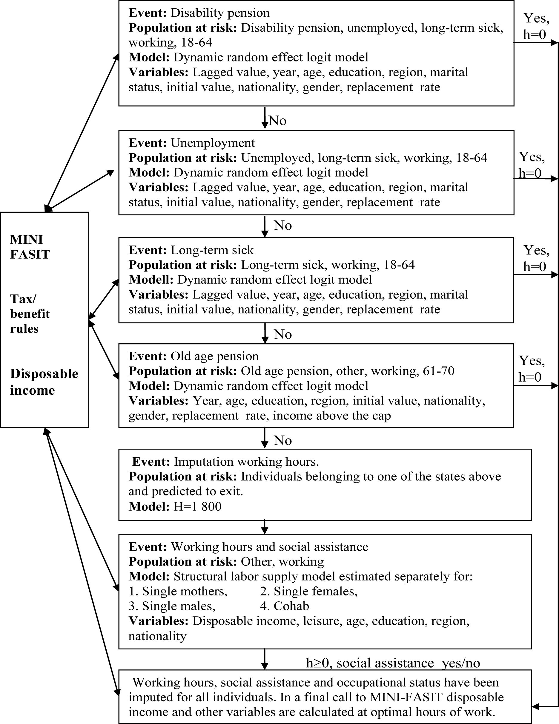

Structure of SWEtaxben.
Figure 1 shows the main sequential steps. The argument in favour of this sequential approach is mainly simplicity but also flexibility since it allows for a separate model for each group. The results regarding the order of the sequence are quite robust. The reason is that most of these group are small (see footnote 5) and therefore the risk that an individual that is predicted in one state would be predicted in another state if the sequence was changed is small. Also, even if the change in sequence had an effect on the number of individuals in different states this would still not have a large impact on disposable income since the benefit levels for most non-work states are similar.
As can be seen, the first step involves the definition of a replacement rate for disability pension. The population at risk (individuals included in the predictions) comprises individuals aged 18–64 (but not older children living with their parents) classified as disabled/unemployed, Long-term sick, or working. For couples, at least one of the spouses must belong to the population at risk. For each individual in this population, the tax/benefit module is called upon to calculate disposable income assuming that everyone is classified as being on full-time disability. Next, for the same individuals, income is calculated assuming full-time work (H=1,800). The ratio of disposable income from disability to disposable income from work defines the replacement rate. For instance, a replacement rate of 0.7 means that an individual who receives full-time compensation from disability insurance receives 70 percent of the disposable income as he/she would have as a full-time worker. A change in a tax/benefit that affects the replacement rate will also affect the probability of entry, staying in, or exiting from disability.
Given the replacement rate, as well as all other explanatory variables included in the model, the probability of disability is calculated. In this calculation, two stochastic terms enter: (1) a random draw from a normal distribution (with an estimated mean and variance) representing individual heterogeneity, and (2) a Monte Carlo experiment. If the simulated probability is less than a random draw from a uniform (0–1) distribution, then the event takes place; that is, the individual is classified as disabled. Individuals not classified as disabled get the temporary status (10) and enter the next stochastic model in the sequence. Note that the random errors for each individual are the same before and after a reform. The Monte Carlo experiment acknowledges the fact that even individuals whose characteristics are such that the likelihood of disability is very low still face the risk of “bad luck.” With appropriate changes, the same argument also applies to an individual with a high systematic probability of disability. This stochastic experiment has been applied to all binary events in the model.
The next step involves unemployment, and the population at risk comprises unemployed, long term sick, and working individuals, as well as those belonging to the temporary status. The steps undertaken are the same as for disability; thus after this step the individuals in the risk population are either classified as unemployed or as being in the temporary state. After this follows the long-term sick module. The population at risk now comprises those who are long-term sick, those who are working, and individuals in the temporary state. Again the same procedure, and as a result of this module, individuals are classified as long-term sick or temporary. The final binary model concerns old-age pension. The population at risk consists of old-age pensioners, other, working, and temporary status aged 61–70. An individual below 61 is not eligible for old-age pension and all individuals older than 70 are by default classified as old-age pensioners. After this step, individuals can also be classified as being in the temporary state.
A simple imputation follows after these binary models. All individuals with the temporary status who before the reform belonged to one of the binary states, i.e., individuals who have exited from one of the binary states without entering another, are imputed as entering the working state and are given a yearly number of working hours of 1,800. This concludes the first part of the model where the binary models are used. Next we will explain the imputation of working hours and social assistance.
All individuals in the risk population (status of other or working) are considered as working or voluntarily non-working. Thus, this is the typical risk population in traditional labour supply studies. For every individual in this population, the tax/benefit module is called upon repeatedly in order to evaluate the budget set. For individuals classified as singles, this requires 14 calls (7 working classes with and without social assistance), and for couples the creation of the budget set requires 98 calls (7*7*2).7 Note that for couples, at least one of the spouses must belong to the population at risk. Given the budget set and all other variables included in the labour supply models, working hours and the probability of social assistance are predicted. The stochastic experiment for those models involves draws from an extreme value distribution. Also, note that different models for predicting labour supply have been applied depending on the family type.
At this stage of the simulation, each individual has a predicted status, number of working hours, and level of welfare participation. A final step is to call the tax/benefit module again to get the predicted disposable income, calculated at the predicted values. Thus, this is the predicted disposable income for the individuals/households resulting from the tax/benefit rules. By changing these rules and repeating the simulation, disposable incomes before and after a reform can be compared.
2.2 Econometric models
The results of the simulations obviously depend on the econometric models and, as mentioned above, four binary models are used to simulate the probability of disability, unemployment, long-term sickness, and old-age pension, and for the conditional labour supply different discrete choice models have been estimated for each family type.
All of the binary models have been estimated as dynamic random-effects logit models. The data used for the estimation is a balanced LINDA panel for the years 2000–2006.
Following Wooldridge (2002, 2005), we define the model as
where
with,
where yit denotes the occupational status of individual i in year t (1 if the individual is disabled, unemployed, etc.), yit−1 is the occupational status in the previous year, and the x variables are measures of observed characteristics, e.g., age and education. Unobserved determinants are time-invariant, μi, or time-variant, εit. The time-invariant component ci is allowed to be correlated with the occupational status of the initial period and the time-average of the explanatory variables. The purpose is to address the initial conditions problem and the possible endogeneity of explanatory variables with respect to timeinvariant characteristics. The x̅ variables denote the average value of the time-invariant variables for each individual. The variables included in the different models are given in Figure 1, but also note that a more detailed description of the estimated models is included in Ericson et al. (2009).
The method used for the conditional labour supply models follows previous work by van Soest (1995); the household model is described in Flood et al. (2004) and the model for the single-headed household in Flood et. al. (2007). These models belong to the class of discrete choice models, and two advantages of this approach are that it allows us to include as many details as needed regarding the budget set and that it extends naturally into a household model, where husbands and wives jointly determine their labour supply.8 9) Specifically, we assume that each individual can choose among seven alternatives in the choice set of income-leisure combinations, and hence the choice set for a household contains 7*7 different hours of work combinations.
We assume that family utility depends not only on consumption and leisure, but also on participation in social assistance. Furthermore, we assume that the utility function is increasing in income and leisure and decreasing in welfare participation. The disutility from participation in social assistance is assumed to reflect the non-monetary costs, such as fixed costs or “stigma,” and is included to account for nonparticipation among eligible families.10
Following van Soest (1995), we use a trans-log specification of the direct utility function, and for any specific household we have
for a single-headed household.
where C is household disposable income as described above, (T-Hj) is leisure (j = M (male) or F (female), and T is an upper limit (4,000). PSA is a binary variable, taking the value one if the household is a receiver of social assistance, and zero otherwise. Dj is also a binary variable, taking the value one if working hours is above zero, reflecting the importance of “fixed cost" of working.
In order to implement the model, we also have to specify the nature of heterogeneity in household preferences and the stochastic disturbances in the utility function. For the household model, heterogeneity in preferences for leisure is introduced as
and in the specification of welfare participation as
The corresponding specifications for the single person are given by
The z-vector includes measurable individual and household characteristics and the ϕ’s represent unobserved variables that affect preferences for leisure. As usual, it is assumed that an important source for population heterogeneity in terms of preferences for leisure is unobserved. In order to account for this, we formulate a finite mixture model that allows for unobserved heterogeneity in a very flexible way without imposing a parametric structure. To make the model estimable, additional random disturbances are added to the utilities of all choice opportunities (for details see Flood et al., 2004 and 2007). Seven different classes or intervals of working hours per year have been used in the estimation: 0, 1–500, 501–1,000, 1,001–1,500, 1,501–2,000, 2,001–2,500, and above 2,500.
Since the parameters in these highly non-linear models do not have a simple interpretation, Table 1 below presents wage elasticities. These are within the bounds typically presented in the literature. Moreover, they are higher for females and there is a negative male-female cross elasticity.
Uncompensated wage elasticities by family type
| Household | Single mothers | Single | Single | ||
|---|---|---|---|---|---|
| Wage increase by 1% | Male | Female | Female | Female | Male |
| Male | 0.10 | −0.07 | 0.05 | ||
| Female | 0 | 0.16 | 0.21 | 0.38 |
3. The social welfare function11
We introduce the idea of a social planner who wants to implement a tax/benefit design to optimize social welfare. The well-known problem of interpersonal comparability is solved by assuming the existence of a common individual welfare function that is assumed to increase in income and leisure. The formal definition of the individual welfare function (ψ) determined by the social planner is given by
where L is leisure and C is disposable income for individual i. The simplest measure of aggregate welfare is the sum of all individuals’ welfare. However, since this implies equal welfare weights to the individuals, independent of the welfare level, this specific welfare function ignores distributive considerations. In order to address distributive justice, individuals with a low welfare should be assigned larger welfare weights than those who are better off. This is described by the following family of rank-dependent welfare functions:
where Ψ1 ≤ Ψ2 ≤ ... ≤ ΨN is the ordered individual welfare levels ψ, and pk(t) is a weight function at percentile t, defined by
The implication of (12) is that the weights given to low-welfare individuals decrease with increasing k. As k → ∞, Wk approaches inequality neutrality and coincides with the linear additive welfare function defined by
To provide a simple guide to understanding the inequality-aversion profiles exhibited by W1, W2, W3, and W∞, Table 2 shows ratios of the corresponding weights – as defined by (12) – of the median individual and the one percent poorest, the five percent poorest, the thirty percent poorest and the five percent richest individual for different social welfare criteria.
Distributional weight profiles of four different social welfare functions
| W1 (Bonferroni) | W2 (Gini) | W3 | W∞ (Utilitarian) | |
|---|---|---|---|---|
| p(.01)/p(.5) | 6.64 | 1.98 | 1.33 | 1 |
| p(.05)/p(.5) | 4.32 | 1.90 | 1.33 | 1 |
| p(.30)/p(.5) | 1.74 | 1.40 | 1.21 | 1 |
| p(.95)/p(.5) | 0.07 | 0.10 | 0.13 | 1 |
The welfare function can be estimated either for households or for individuals. In either case, the problem of comparing single- and non-single households must be solved. In Aaberge et al. (2008), the welfare measure is based on individuals and in order to make individuals in couple and single households comparable, the disposable income of the couple is divided by the square root of two. In this study, we choose the household as the unit for estimation and welfare evaluation. We do this by transforming a couple-household into one representative household by using the average of disposable income (C) and working hours (H). Further, in order to compensate for number of children, we divide household disposable income by the square root of one plus the number of children.12 A discrete choice translog model,
is then estimated on a sample of households younger than 70 (average age used for couples). Thus, this is a simplified version of the labour supply model described above and as in that model T=4 and hours H are divided by 1,000 and income C by 100,000. The estimated parameters are presented in Table 3.
Estimated parameters of the social welfare function
| Estimates | Standard Errors | |
|---|---|---|
| Log leisure, βl | 3.0985 | 0.0215 |
| Log leisure squared, βll | 0.3620 | 0.0151 |
| Log income, βC | 4.7262 | 0.0224 |
| Log income squared, βCC | −0.0616 | 0.0089 |
These parameters produce a welfare function that is increasing in leisure and income.
The next section describes the use of the social welfare function in order to identify an optimal tax/benefit design.
4. Choosing the optimal tax
As a start, consider the following steps for a given tax/benefit system:
SWEtaxben provides us with a set of optimal (preferred) hours and consumption for each individual in the sample.
At these optimal hours and consumption, the household’s social welfare function is evaluated for each of the four choices of inequality-aversion discussed above.
Repeat these steps for a large number of alternative tax/benefit systems; the one that produces the highest aggregate welfare is referred to as the optimal tax/benefit system. Of course this is done for each of the four variants of the welfare functions, and it cannot be expected that these produce the same optimal design. For this reason the results for all four welfare measures have to be presented.
In order to make a welfare comparison meaningful, we have to impose budget neutrality. Thus, for most of the reforms suggested, we impose the restriction that they must produce the same central governmental budget. Neutrality is obtained by adjusting the (proportional) municipal tax rate. Since this tax corresponds to such a large part of the total tax revenue (in 2006 the tax rate varied across municipalities from 28.89 to 34.24 percent of taxable income), it typically requires minor changes in order to achieve neutrality. However, even if neutrality is imposed when calculating the welfare measures, it is still interesting to record what effect a reform would have on the budget and tax revenues as well as on the initial labour supply and income without imposing neutrality, and hence this will be presented as part of the results.
Before presenting the different tax and benefit systems that are included in the evaluation, it seems appropriate to give a short description of historical tax rates as well as of the system in the reference year 2006.
5. Swedish income taxes and benefits a background
5.1 Income taxes
Since the early 1980s, several tax reforms have been implemented. The most important one was introduced in 1991, and its main characteristics were a decrease in income taxes, a broadening of the tax base, and an introduction of a dual income tax system with a proportional tax on capital (30%). From 1991, the income tax system has undergone several changes but has still kept much of its basic post-reform structure. However, an important change was made in 2007, when an in-work tax credit was introduced. The tax credit was reinforced during 2008 and further in 2009 when also the national (central governmental) tax was lowered.
In the beginning of the 1980s, the Swedish income tax system was known for its high level, large number of brackets, and high degree of progressivity. Today, a low- and medium-income earner pays an income tax similar to the average overall OECD level (OECD, 2007). The municipal and national taxes, as a share of earnings, have decreased by almost 10 percentage points since 1980. Despite the income tax cuts, the tax ratio, measured as total taxes in relation to GNP, is still among the very highest in the OECD area. However, when comparing tax ratios one should bear in mind that transfer incomes like pensions and sickness benefits are regarded as taxable incomes in Sweden. Lower taxes on earnings and a relatively stable tax ratio imply large changes in the tax mix. From an OECD perspective, Sweden is more dependent on income taxes and payroll fees and less on consumption taxes compared to an average OECD country.

The Swedish income tax in 2006.
Note: taxes are evaluated at an average municipal tax rate (31.44%). The axis on the left hand side shows marginal and average tax rates and the axis on the right hand side refers to the income distribution.
In this study we use as a point of reference the tax system in 2006 as depicted in Figure 2. The Swedish income tax system consists of two parts: a flat municipal tax and a progressive national tax regime. The individual is the taxation-unit and income taxes are independent of marital status. The flat municipal tax rate varies across municipalities; in 2006 it ranged from 28.89 to 34.24 percent with an average of 31.55 percent. The marginal taxes have an irregular shape up to SEK 320,000, the first breaking point for national tax. This shape is explained by the phase-in and phase-out of a basic tax deduction. The national tax rate is 20 percent from the first breaking point up to the second at SEK 470,000 and 25 percent above that. The distribution of gross (taxable) income shows that most individuals face a marginal tax rate close to the municipal tax rate, and about 22 percent reach the first breaking point for national taxes and only about 7 percent pay the highest rate.
5.2 Child and housing allowance
Child and housing allowance are included in the evaluation. All children who live in Sweden are entitled to child allowance. The child allowance is SEK 1,050 per child per month. This monthly, tax-free allowance is paid until the child reaches the age of 16. After 16, children in full-time education are entitled to a study allowance. Special large family supplement is paid to families with two or more children.
Housing allowance is determined by nation-wide benefit rules. Eligibility for the benefit depends on household income, cost for housing, and the size of the household. The allowance is reduced above an income of SEK 117,000 per year for singles and for married persons and partners the corresponding limit is 58,500 each. The upper limit for receiving the allowance is a household income of SEK 408,000 per year.
6. Selection of tax and benefit systems
Aaberge and Colombino approximated the Norwegian income tax system by a piece-wise tax function allowing for four brackets and six parameters, and then searched over the parameter space to find an “optimal" income tax. Even if this is an efficient way to select among different designs, an alternative approach is used in the present paper. Since we focus on realistic tax systems in the sense that they are politically/economically credible, a discretionary approach is used. To describe all our tax/benefits reform by the approach used in Aaberge and Colombino should not be possible, as we consider changes in the benefit system and introduce an age-dependent tax system.
As mentioned above, the tax/benefit system in 2006 is taken as a reference, and based on this system a combination of the following changes are evaluated:
National taxes; changes in levels, breaking points, and highest bracket.
Basic deduction and in-work tax credit.
Child and housing allowances.
In addition to these changes, the evaluation also includes
Flat tax.
Finally two designs inspired by the optimal tax literature are included:
An age-dependent tax.
Zero marginal tax rate at the highest income.
The flat as well as the age-dependent taxes will be evaluated without imposing the neutrality constraints. The reason is that these taxes are proportional, and the method in this paper for imposing neutrality by changing another proportional tax is not meaningful. Obviously, other criteria than welfare measures are more important in order to characterize the properties of these reforms. The presentation below starts with the results for the flat tax, followed by the results for an age-dependent tax and zero tax at the highest income. After this follows an evaluation of the optimal combinations of tax and benefit changes.
7. Results
7.1 Flat tax
A flat tax has been part of the international tax debate for many years, e.g., Hall and Rabushka (1985, 1995), and it is also a tax that has been implemented or is in the process of being implemented in a number of countries, especially in the East European so-called transitional countries. However, in real life many different designs have been implemented, sometimes with a uniform tax rate for business and personal income and other times with a lower tax-free allowance for personal income. Even if a flat tax is discussed in the current public debate, it does not seem to be part of the current debate within the OECD area. Instead a progressive system combined with an in-work tax credit seems to be the norm; see Messere, Kam, and Heady (2006).
Despite the current debate, there are a number of arguments in favor of a flat tax, such as simplicity and long-run effects on economic growth. Here, simplicity should not be regarded in the myopic sense of just producing simple rules for income taxation, but rather in a general sense. A flat tax on labour income at a rate harmonizing with the capital levy would help reduce the classical conflict in a dual income tax system caused by different tax rates for capital and labour. This raises an important shortcoming of income taxation studies: the question of optimal taxation should be generalized to the whole tax system and not only taxation of labour, i.e., the whole tax mix should be included in the analyses. However, this would obviously require an extremely complicated simulation model. It is at any rate important to realize that a flat tax has several potential advantages that are not credited in this study, e.g., the possibility to reduce the incentive to move income to the source with the lowest taxation and desirable long-run effects on economic growth. As mentioned above in the evaluation of the flat tax, budget neutrality is not imposed and instead the evaluation focuses on other dimensions than welfare. Thus, the welfare measures are not included in Table 4.
Flat tax.
| Reform | Description | Hours | Participation | Budget | Disposable income | Labor income | Income tax | GINI | D9/D2 |
|---|---|---|---|---|---|---|---|---|---|
| 0 | Base 2006 | 0.00% | 0.00% | 0.00% | 0.00% | 0.00% | 0.00% | 0.0% | 2.34 |
| 1 | 20% | 4.78% | 1.55% | −10.28% | 17.35% | 4.88% | −30.93% | 8.2% | 2.84 |
| 2 | 21% | 4.60% | 1.44% | −9.13% | 15.99% | 4.72% | −27.99% | 8.3% | 2.81 |
| 3 | 22% | 4.41% | 1.34% | −7.98% | 14.62% | 4.55% | −25.07% | 8.5% | 2.77 |
| 4 | 23% | 4.18% | 1.21% | −6.86% | 13.23% | 4.36% | −22.16% | 8.6% | 2.74 |
| 5 | 24% | 3.95% | 1.09% | −5.75% | 11.86% | 4.16% | −19.26% | 8.8% | 2.70 |
| 6 | 25% | 3.69% | 0.95% | −4.66% | 10.47% | 3.95% | −16.39% | 9.0% | 2.67 |
| 7 | 26% | 3.43% | 0.82% | −3.57% | 9.09% | 3.73% | −13.52% | 9.2% | 2.63 |
| 8 | 27% | 3.18% | 0.67% | −2.50% | 7.71% | 3.51% | −10.67% | 9.4% | 2.60 |
| 9 | 28% | 2.89% | 0.50% | −1.44% | 6.32% | 3.27% | −7.83% | 9.7% | 2.57 |
| 10 | 29% | 2.61% | 0.32% | −0.40% | 4.95% | 3.04% | −5.01% | 9.9% | 2.53 |
| 11 | 30% | 2.29% | 0.12% | 0.61% | 3.56% | 2.77% | −2.21% | 10.1% | 2.50 |
| 12 | 31% | 1.98% | −0.08% | 1.64% | 2.18% | 2.51% | 0.58% | 10.4% | 2.46 |
| 13 | 32% | 1.67% | −0.27% | 2.64% | 0.80% | 2.24% | 3.35% | 10.6% | 2.43 |
| 14 | 33% | 1.32% | −0.49% | 3.61% | −0.56% | 1.96% | 6.11% | 10.9% | 2.40 |
| 15 | 34% | 0.95% | −0.73% | 4.55% | −1.94% | 1.65% | 8.83% | 11.2% | 2.36 |
| 16 | 35% | 0.60% | −0.95% | 5.52% | −3.30% | 1.38% | 11.56% | 11.4% | 2.33 |
Table 4 summarizes the results. The first row, denoted reform 0, displays the results for the base year, i.e., for the tax/benefit rules in 2006. Since most results are presented as percentage change relative to the base year, most of the entries are zero, except the income distribution D9/D2 (decile 9 / decile 2). Thus, at the base year, the ratio D9/D2 was 2.34, i.e., the median disposable income in decile 9 was 2.34 higher than the median income in decile 2.
Our evaluation covers a flat tax in the range from 20 to 35 percent. As follows from Table 4, a 20 percent flat tax rate has a strong positive effect on working hours (almost 5%) and therefore also on disposable income (more than 17 percent). Even if labour income increases by almost 5 percent, this is not enough to compensate for reduced taxes (a drop of more than 30 percent). Of course, it can be argued that a tax rate of 20 percent is not a realistic alternative, but as a contrast a 30 percent tax is budget neutral and a 25 percent tax entails a budget deficit of less than 5 percent. Since all comparisons are made according to the rules in 2006, i.e., before the introduction of the in-work tax credit, the budget deficit would be much smaller if comparing with the 2009 budget when the in-work tax credit was implemented. Using SWEtaxben for the comparison of a flat tax and the 2009 tax year shows that a 25 percent flat tax is almost budget neutral (not shown in Table 4), a result that confirms earlier findings; see Lundgren et al. (2008).
A flat tax of 25 percent would certainly affect the income distribution. According to our simulations, the Gini coefficient increases by 9 percent (compared to 2006) and the D9/D2 ratio increases from 2.34 to 2.67. One explanation to the modest increase in the inequality of income is the increase in participation. A low flat tax decreases the replacement rate and increases the probability of participation, and, in contrast to an in-work tax credit, the flat tax also increases working hours for median- and high-income earners.
To conclude, a flat tax has several interesting properties, yet the disadvantage in terms of increasing income inequality will have a large negative impact in an evaluation based on social welfare.
7.2 Age-dependent tax
A basic theme in optimal taxation is that a tax should be related to the ability to pay. It is not income, as such, that should be taxed but the ability to earn income. It is of course difficult to implement a tax based on an unobservable such as ability. However, the crucial idea is that a tax should be related to an exogenous factor that does not produce any negative incentives. As an attempt to catch the basic idea of taxation based on an exogenous factor, we suggest a tax that is age dependent. Thus, age is used as a proxy for ability.
The interest in an age dependent tax has recently been addressed in Banks and Diamond (2010) who argue that age dependence is one of the most promising areas for a tax reform. A strong argument in favor of such reform is also presented in Weinzierl (2010). In real life such designs are not new. For instance, the current Swedish system includes an age component. The in-work tax credit has a special and much more generous level for people older than 65. Further, employers’ social security contributions are lower for younger and older people.
Two alternatives of an age-dependent tax are evaluated: (1) a generalization of the prevailing age-dependent in-work tax credit, with a higher level for those younger than 25 and older than 61; and (2) a scheme where individuals younger than 26 and older than 65 pay a flat tax of 15 percent, and from 26 years of age the tax increases by a constant up to the age of 45 and then decreases by the same constant until the age of 65. The shape of this profile, from 26 to 65 years of age, is thus an inverted V, with the peak at the age of 45. Constants from one to two percent per year are used in the phase-in and phase-out regions, where one (two) percent implies a highest tax rate (at age 45) of 35 (55) percent. Note that in this evaluation as well as in the flat tax evaluation, the basic deduction and the national and the municipal taxes are set to zero. Also, since budget neutrality is not imposed, the welfare measures are not included in the table.
Age-dependent taxes.
| Reform | Flat tax | Up 26–46 (%) | Down 46–65 (%) | Hours | Participation | Budget | Disposabl e-income | Labor income | Income tax | GINI | D9/D2 |
|---|---|---|---|---|---|---|---|---|---|---|---|
| 0 | Base 2006 | 0.00% | 0.00% | 0.00% | 0.00% | 0.00% | 0.00% | 0.0% | 2.34 | ||
| 1 | 15% | 1.00 | 1.00 | 3.89% | 1.11% | −6.60% | 12.46% | 4.02% | −21.12% | 6.6% | 2.68 |
| 2 | 15% | 1.05 | 1.05 | 3.77% | 1.05% | −6.15% | 11.87% | 3.92% | −19.93% | 6.6% | 2.67 |
| 3 | 15% | 1.10 | 1.10 | 3.65% | 0.98% | −5.71% | 11.28% | 3.81% | −18.74% | 6.6% | 2.65 |
| 4 | 15% | 1.15 | 1.15 | 3.53% | 0.92% | −5.27% | 10.70% | 3.71% | −17.56% | 6.7% | 2.63 |
| 5 | 15% | 1.20 | 1.20 | 3.40% | 0.85% | −4.85% | 10.10% | 3.59% | −16.39% | 6.8% | 2.62 |
| 6 | 15% | 1.25 | 1.25 | 3.26% | 0.77% | −4.43% | 9.51% | 3.47% | −15.23% | 6.9% | 2.60 |
| 7 | 15% | 1.30 | 1.30 | 3.11% | 0.68% | −4.02% | 8.91% | 3.33% | −14.08% | 7.0% | 2.59 |
| 8 | 15% | 1.35 | 1.35 | 2.97% | 0.60% | −3.60% | 8.33% | 3.22% | −12.92% | 7.1% | 2.57 |
| 9 | 15% | 1.40 | 1.40 | 2.83% | 0.52% | −3.19% | 7.74% | 3.09% | −11.77% | 7.2% | 2.56 |
| 10 | 15% | 1.45 | 1.45 | 2.66% | 0.42% | −2.81% | 7.14% | 2.94% | −10.65% | 7.3% | 2.54 |
| 11 | 15% | 1.50 | 1.50 | 2.50% | 0.32% | −2.43% | 6.55% | 2.80% | −9.52% | 7.5% | 2.52 |
| 12 | 15% | 1.55 | 1.55 | 2.33% | 0.21% | −2.05% | 5.96% | 2.65% | −8.41% | 7.7% | 2.51 |
| 13 | 15% | 1.60 | 1.60 | 2.18% | 0.13% | −1.65% | 5.38% | 2.52% | −7.27% | 7.8% | 2.49 |
| 14 | 15% | 1.65 | 1.65 | 1.99% | 0.00% | −1.30% | 4.78% | 2.35% | −6.19% | 8.0% | 2.48 |
| 15 | 15% | 1.70 | 1.70 | 1.81% | −0.12% | −0.94% | 4.19% | 2.19% | −5.09% | 8.2% | 2.47 |
| 16 | 15% | 1.75 | 1.75 | 1.58% | −0.27% | −0.63% | 3.58% | 1.98% | −4.05% | 8.5% | 2.45 |
| 17 | 15% | 1.80 | 1.80 | 1.36% | −0.43% | −0.32% | 2.98% | 1.79% | −3.00% | 8.7% | 2.44 |
| 18 | 15% | 1.85 | 1.85 | 1.16% | −0.56% | 0.02% | 2.39% | 1.62% | −1.94% | 9.0% | 2.42 |
| 19 | 15% | 1.90 | 1.90 | 0.93% | −0.72% | 0.32% | 1.80% | 1.42% | −0.90% | 9.3% | 2.42 |
| 20 | 15% | 1.95 | 1.95 | 0.73% | −0.85% | 0.65% | 1.22% | 1.25% | 0.15% | 9.5% | 2.40 |
| 21 | 15% | 2.00 | 2.00 | 0.50% | −1.00% | 0.94% | 0.63% | 1.05% | 1.16% | 9.8% | 2.39 |
| 22 | Extended 2009 in-work tax credit | 1.79% | 1.52% | −3.93% | 5.76% | 1.38% | −11.55% | −1.4% | 2.48 | ||
The results are presented in Table 5, where the first row shows the base year 2006, the last row the generalized age-dependent in-work tax credit, and the rows in between different constants for the phase-in and phase-out regions. As expected, the lowest scale factor results in a large budget deficit, but it also has the largest increase in working hours of all reforms evaluated in this study. Number of working hours increases by almost 4 percent and participation by more than 1 percent. Obviously, this results in a dramatic increase of labour income. Despite these strong behavioural effects, there is a large decrease in tax revenues, but (due to behavioural effects) the central government’s budget deficit is much smaller (6.6 %) due to lower social expenditures and increased revenues from payroll taxes and VAT. A purely age-based tax affects the income distribution – the Gini coefficient increases by about 7 percent. Increasing the phase-in and phase-out constant reduces disposable income but also increases tax revenues.
Compared to the inverted V tax, the age-dependent in-work tax credit performs relatively well. As expected, the increase in participation is significant but the effect on the intensive margin is not as large. The budget deficit increases by about 4 percent, but, as expected, with a less dispersed income distribution. This shows the important effect an in-work.tax credit has on the participation decision and an increased participation implies less income inequality.
7.3 Zero tax on the highest income
As mentioned earlier, this reform is inspired by the optimal tax theory and obtained by setting the marginal tax rate to zero at the highest income (according to the theory at highest ability; see Seade, 1977).13 The intuition behind this result is that a nonzero marginal tax rate distorts the labour supply of the highest-ability person. If this tax rate were changed to zero, the highest-ability person might choose to work more, which increases his welfare. However, the tax revenue would not change, because before the tax change this labour is not provided, and with a zero tax rate, the extra labour supply is not taxed. This argument applies only to incomes above the highest observable, since changes in marginal tax rates below this level affect the taxes paid by people with higher incomes. Unfortunately, this result does not give any information about the marginal tax level just below the top of the income distribution.
Admittedly, the implementation of this theory is far from obvious and we choose to evaluate this reform at different “highest incomes,” starting at one million SEK and then increasing it up to ten million. As expected the effects on labour supply, income, and taxes are almost negligible. The largest effect is of course obtained when the upper limit is set to one million SEK – working hours and disposable income increase by 0.08 percent and 0.5 percent, respectively, and tax revenues decrease by 0.8 percent.
7.4 Summary of results regarding flat and age dependent tax designs
To summarize the results so far, a flat tax or an age-dependent tax has some advantages: simplicity and efficiency. At low tax levels, both the flat and age-dependent designs have strong labour supply effects. A low tax at the start and at the end of the working life creates incentives for both the entry and exit decision. The simple inverted V tax using a one percent phase-in/phase-out factor implies increased labour supply of almost four percent; however the predicted budget deficit is almost 7 percent. A flat tax of 23 percent produces almost the same budget deficit but has slightly larger labour supply effects. Comparing the budget neutral rates gives a 1.85 percent phase-in/phase-out factor for the age dependent design compared to 29 percent for the flat tax. The disadvantage of both designs is an increased income inequality, although for the age dependent tax this increase is slightly smaller. However, as already mentioned budget neutrality is not imposed.
The increase in inequality raises the issue of compensation for low-income households. This also raises the issue of combined tax/benefit designs, providing a link to the next subsection, which evaluates the optimal combination of tax/benefits.
7.5 Combined reforms
The tax/benefits that are included in the combined designs are: the national tax at the highest level (above the second break point), the national tax (both the level and the location of the first breaking point), the basic deduction, the in-work tax credit, and finally housing allowance.14 The in-work tax credit also includes the age-dependent design mentioned above. We have evaluated hundreds of tax/benefit schemes, with several levels of each factor. To save space, we have chosen to present a selection of the schemes that remain after a first sorting out to find an optimal reform. The reforms are ranked according to the highest average welfare over all four welfare measures.
Combination of tax/benefits15.
| Reform | Top level | Level | Break point | Housing allowance | Credit/deduction | Hours | Participation | Budget | Disposable income | Labor income | Income tax | GINI | D9/D2 | W1 | W2 | W3 | W∞ |
|---|---|---|---|---|---|---|---|---|---|---|---|---|---|---|---|---|---|
| 0 | 0% | 0% | 0% | 0% | 2006 | 0.00% | 0.00% | 0.00% | 0.00% | 0.00% | 0.00% | 0.0% | 2.34 | 80 | 80 | 80 | 76 |
| 39 | 0% | -25% | 25% | 50% | 2009 + age | 2.69% | 1.54% | −4.85% | 8.31% | 2.49% | −14.97% | 1.6% | 2.46 | 17 | 3 | 1 | 4 |
| 79 | −100% | −25% | 25% | 50% | 2009 + age | 2.74% | 1.54% | −4.85% | 8.46% | 2.58% | −15.11% | 2.1% | 2.47 | 21 | 5 | 2 | 2 |
| 59 | −100% | 0% | 25% | 50% | 2009 + age | 2.54% | 1.53% | −4.76% | 7.90% | 2.27% | −14.48% | 0.9% | 2.45 | 18 | 6 | 3 | 6 |
| 77 | −100% | −25% | 25% | 50% | 2009 +50% | 3.06% | 1.91% | −7.51% | 11.40% | 2.80% | −21.75% | 1.1% | 2.47 | 12 | 7 | 5 | 21 |
| 19 | 0% | 0% | 25% | 50% | 2009 + age | 2.49% | 1.53% | −4.76% | 7.72% | 2.16% | −14.31% | 0.3% | 2.45 | 22 | 9 | 4 | 13 |
| 37 | 0% | −25% | 25% | 50% | 2009 +50% | 3.03% | 1.91% | −7.48% | 11.27% | 2.73% | −21.61% | 0.7% | 2.47 | 11 | 8 | 6 | 24 |
| 69 | −100% | −25% | 0% | 50% | 2009 + age | 2.18% | 1.46% | −4.47% | 7.21% | 2.00% | −13.40% | 1.0% | 2.42 | 16 | 10 | 9 | 14 |
| 29 | 0% | −25% | 0% | 50% | 2009 + age | 2.10% | 1.46% | −4.44% | 6.96% | 1.84% | −13.14% | 0.3% | 2.42 | 13 | 11 | 12 | 18 |
| 78 | −100% | −25% | 25% | 50% | 2009 +100% | 3.52% | 2.35% | −10.60% | 14.87% | 3.11% | −29.50% | 0.1% | 2.48 | 1 | 1 | 11 | 46 |
| 38 | 0% | −25% | 25% | 50% | 2009 +100% | 3.49% | 2.36% | −10.57% | 14.74% | 3.05% | −29.35% | −0.3% | 2.48 | 2 | 2 | 13 | 50 |
| 57 | −100% | 0% | 25% | 50% | 2009 +50% | 2.88% | 1.90% | −7.40% | 10.87% | 2.52% | −21.14% | −0.1% | 2.45 | 15 | 16 | 16 | 31 |
| 67 | −100% | −25% | 0% | 50% | 2009 +50% | 2.55% | 1.84% | −7.12% | 10.23% | 2.27% | −20.11% | 0.0% | 2.42 | 9 | 14 | 20 | 35 |
| 34 | 0% | −25% | 25% | 0% | 2009 + age | 2.82% | 1.64% | −4.66% | 8.29% | 2.59% | −14.92% | 1.7% | 2.47 | 51 | 22 | 7 | 3 |
| 58 | −100% | 0% | 25% | 50% | 2009 +100% | 3.36% | 2.35% | −10.48% | 14.37% | 2.87% | −28.89% | −1.0% | 2.47 | 3 | 4 | 18 | 59 |
| 74 | −100% | −25% | 25% | 0% | 2009 + age | 2.86% | 1.64% | −4.67% | 8.43% | 2.68% | −15.05% | 2.1% | 2.47 | 52 | 25 | 8 | 1 |
| 54 | −100% | 0% | 25% | 0% | 2009 + age | 2.66% | 1.62% | −4.58% | 7.87% | 2.37% | −14.42% | 0.9% | 2.45 | 48 | 24 | 10 | 5 |
| 64 | −100% | −25% | 0% | 0% | 2009 + age | 2.32% | 1.57% | −4.27% | 7.19% | 2.11% | −13.34% | 1.0% | 2.42 | 41 | 26 | 15 | 12 |
| 27 | 0% | −25% | 0% | 50% | 2009 +50% | 2.47% | 1.84% | −7.10% | 9.98% | 2.12% | −19.86% | −0.7% | 2.42 | 10 | 17 | 25 | 43 |
| 17 | 0% | 0% | 25% | 50% | 2009 +50% | 2.82% | 1.89% | −7.41% | 10.70% | 2.40% | −20.98% | −0.6% | 2.45 | 19 | 19 | 24 | 36 |
| 73 | −100% | −25% | 25% | 0% | 2009 +100% | 3.62% | 2.43% | −10.44% | 14.84% | 3.20% | −29.47% | 0.2% | 2.48 | 25 | 18 | 19 | 39 |
| 24 | 0% | −25% | 0% | 0% | 2009 + age | 2.23% | 1.56% | −4.25% | 6.93% | 1.96% | −13.08% | 0.3% | 2.42 | 42 | 28 | 17 | 16 |
| 14 | 0% | 0% | 25% | 0% | 2009 + age | 2.61% | 1.63% | −4.58% | 7.70% | 2.26% | −14.26% | 0.4% | 2.45 | 54 | 30 | 14 | 10 |
| 49 | −100% | 0% | 0% | 50% | 2009 + age | 1.79% | 1.44% | −4.28% | 6.27% | 1.49% | −12.28% | −0.6% | 2.39 | 23 | 23 | 32 | 32 |
| 36 | 0% | −25% | 25% | 50% | 2009 | 2.48% | 1.30% | −4.47% | 7.75% | 2.33% | −13.82% | 1.9% | 2.46 | 37 | 38 | 26 | 11 |
| 76 | −100% | −25% | 25% | 50% | 2009 | 2.52% | 1.30% | −4.47% | 7.89% | 2.42% | −13.95% | 2.3% | 2.47 | 38 | 40 | 27 | 8 |
| 18 | 0% | 0% | 25% | 50% | 2009 +100% | 3.31% | 2.35% | −10.48% | 14.20% | 2.75% | −28.74% | −1.4% | 2.46 | 6 | 13 | 29 | 66 |
| 68 | −100% | −25% | 0% | 50% | 2009 +100% | 3.06% | 2.30% | −10.21% | 13.76% | 2.63% | −27.93% | −1.0% | 2.44 | 4 | 12 | 30 | 68 |
| 33 | 0% | −25% | 25% | 0% | 2009 +100% | 3.59% | 2.43% | −10.42% | 14.71% | 3.13% | −29.32% | −0.2% | 2.48 | 26 | 20 | 23 | 48 |
| 72 | −100% | −25% | 25% | 0% | 2009 +50% | 3.19% | 2.01% | −7.33% | 11.38% | 2.90% | −21.71% | 1.1% | 2.47 | 47 | 33 | 21 | 19 |
| 32 | 0% | −25% | 25% | 0% | 2009 +50% | 3.16% | 2.02% | −7.30% | 11.26% | 2.84% | −21.56% | 0.7% | 2.47 | 46 | 34 | 22 | 22 |
| 28 | 0% | −25% | 0% | 50% | 2009 +100% | 2.98% | 2.30% | −10.17% | 13.53% | 2.50% | −27.67% | −1.6% | 2.44 | 5 | 15 | 34 | 72 |
| 56 | −100% | 0% | 25% | 50% | 2009 | 2.32% | 1.29% | −4.39% | 7.34% | 2.11% | −13.32% | 1.1% | 2.45 | 36 | 43 | 31 | 17 |
| 9 | 0% | 0% | 0% | 50% | 2009 + age | 1.69% | 1.45% | −4.25% | 5.95% | 1.30% | −11.95% | −1.4% | 2.39 | 24 | 31 | 40 | 45 |
| 66 | −100% | −25% | 0% | 50% | 2009 | 1.96% | 1.22% | −4.10% | 6.65% | 1.84% | −12.25% | 1.2% | 2.42 | 32 | 45 | 39 | 26 |
| 52 | −100% | 0% | 25% | 0% | 2009 +50% | 3.01% | 2.00% | −7.22% | 10.86% | 2.63% | −21.09% | 0.0% | 2.46 | 49 | 37 | 28 | 29 |
| 53 | −100% | 0% | 25% | 0% | 2009 +100% | 3.47% | 2.43% | −10.32% | 14.35% | 2.95% | −28.86% | −0.9% | 2.47 | 28 | 27 | 33 | 56 |
| 16 | 0% | 0% | 25% | 50% | 2009 | 2.27% | 1.29% | −4.38% | 7.16% | 2.00% | −13.16% | 0.5% | 2.45 | 39 | 48 | 35 | 23 |
| 47 | −100% | 0% | 0% | 50% | 2009 +50% | 2.18% | 1.81% | −6.95% | 9.32% | 1.77% | −19.04% | −1.5% | 2.40 | 14 | 29 | 48 | 61 |
| 26 | 0% | −25% | 0% | 50% | 2009 | 1.87% | 1.22% | −4.07% | 6.39% | 1.68% | −11.99% | 0.5% | 2.42 | 33 | 49 | 43 | 28 |
| 62 | −100% | −25% | 0% | 0% | 2009 +50% | 2.69% | 1.95% | −6.93% | 10.21% | 2.38% | −20.06% | 0.0% | 2.43 | 44 | 41 | 36 | 34 |
| 48 | −100% | 0% | 0% | 50% | 2009 +100% | 2.72% | 2.28% | −10.03% | 12.89% | 2.17% | −26.89% | −2.4% | 2.41 | 7 | 21 | 52 | 77 |
| 44 | −100% | 0% | 0% | 0% | 2009 + age | 1.92% | 1.54% | −4.09% | 6.24% | 1.60% | −12.22% | −0.6% | 2.39 | 50 | 44 | 38 | 30 |
| 63 | −100% | −25% | 0% | 0% | 2009 +100% | 3.16% | 2.38% | −10.04% | 13.73% | 2.72% | −27.90% | −0.9% | 2.44 | 27 | 32 | 44 | 65 |
| 31 | 0% | −25% | 25% | 0% | 2009 | 2.63% | 1.42% | −4.27% | 7.73% | 2.45% | −13.75% | 1.9% | 2.47 | 61 | 58 | 41 | 9 |
| 22 | 0% | −25% | 0% | 0% | 2009 +50% | 2.61% | 1.95% | −6.91% | 9.97% | 2.23% | −19.81% | −0.6% | 2.42 | 45 | 46 | 42 | 41 |
| 13 | 0% | 0% | 25% | 0% | 2009 +100% | 3.41% | 2.42% | −10.32% | 14.17% | 2.84% | −28.70% | −1.4% | 2.47 | 31 | 35 | 45 | 64 |
| 12 | 0% | 0% | 25% | 0% | 2009 +50% | 2.96% | 2.00% | −7.23% | 10.68% | 2.51% | −20.93% | −0.5% | 2.45 | 56 | 50 | 37 | 33 |
| 71 | −100% | −25% | 25% | 0% | 2009 | 2.67% | 1.42% | −4.27% | 7.88% | 2.54% | −13.89% | 2.3% | 2.47 | 63 | 59 | 47 | 7 |
| 51 | −100% | 0% | 25% | 0% | 2009 | 2.47% | 1.41% | −4.19% | 7.32% | 2.23% | −13.26% | 1.1% | 2.45 | 59 | 57 | 46 | 15 |
| 7 | 0% | 0% | 0% | 50% | 2009 +50% | 2.06% | 1.81% | −6.94% | 9.00% | 1.57% | −18.74% | −2.3% | 2.39 | 20 | 39 | 56 | 71 |
| 23 | 0% | −25% | 0% | 0% | 2009 +100% | 3.09% | 2.38% | −10.00% | 13.50% | 2.59% | −27.63% | −1.5% | 2.44 | 30 | 36 | 51 | 70 |
| 46 | −100% | 0% | 0% | 50% | 2009 | 1.56% | 1.20% | −3.92% | 5.70% | 1.32% | −11.13% | −0.4% | 2.39 | 35 | 53 | 57 | 44 |
| 11 | 0% | 0% | 25% | 0% | 2009 | 2.42% | 1.41% | −4.19% | 7.14% | 2.11% | −13.10% | 0.6% | 2.45 | 60 | 60 | 50 | 20 |
| 8 | 0% | 0% | 0% | 50% | 2009 +100% | 2.61% | 2.28% | −10.02% | 12.59% | 1.97% | −26.61% | −3.2% | 2.41 | 8 | 42 | 61 | 80 |
| 4 | 0% | 0% | 0% | 0% | 2009 + age | 1.82% | 1.55% | −4.07% | 5.92% | 1.40% | −11.90% | −1.4% | 2.39 | 55 | 51 | 49 | 37 |
| 61 | −100% | −25% | 0% | 0% | 2009 | 2.12% | 1.35% | −3.89% | 6.64% | 1.96% | −12.18% | 1.2% | 2.42 | 57 | 61 | 54 | 25 |
| 21 | 0% | −25% | 0% | 0% | 2009 | 2.03% | 1.34% | −3.86% | 6.38% | 1.81% | −11.92% | 0.5% | 2.42 | 58 | 62 | 55 | 27 |
| 42 | −100% | 0% | 0% | 0% | 2009 +50% | 2.31% | 1.91% | −6.77% | 9.29% | 1.88% | −19.00% | −1.5% | 2.40 | 43 | 52 | 53 | 58 |
| 43 | −100% | 0% | 0% | 0% | 2009 +100% | 2.83% | 2.36% | −9.86% | 12.87% | 2.27% | −26.85% | −2.3% | 2.42 | 29 | 47 | 58 | 75 |
| 6 | 0% | 0% | 0% | 50% | 2009 | 1.47% | 1.21% | −3.89% | 5.39% | 1.14% | −10.81% | −1.2% | 2.39 | 40 | 56 | 60 | 55 |
| 41 | −100% | 0% | 0% | 0% | 2009 | 1.71% | 1.32% | −3.72% | 5.68% | 1.44% | −11.07% | −0.4% | 2.39 | 62 | 63 | 62 | 40 |
| 3 | 0% | 0% | 0% | 0% | 2009 +100% | 2.72% | 2.36% | −9.86% | 12.56% | 2.06% | −26.57% | −3.1% | 2.41 | 34 | 54 | 63 | 79 |
| 2 | 0% | 0% | 0% | 0% | 2009 +50% | 2.19% | 1.91% | −6.76% | 8.98% | 1.68% | −18.70% | −2.3% | 2.39 | 53 | 55 | 59 | 69 |
| 1 | 0% | 0% | 0% | 0% | 2009 | 1.61% | 1.33% | −3.69% | 5.37% | 1.25% | −10.75% | −1.2% | 2.39 | 64 | 64 | 64 | 52 |
| 55 | −100% | 0% | 25% | 50% | 2006 | 0.68% | −0.07% | −0.70% | 1.96% | 0.85% | −2.55% | 2.5% | 2.41 | 67 | 65 | 65 | 53 |
| 75 | −100% | −25% | 25% | 50% | 2006 | 0.88% | −0.06% | −0.79% | 2.52% | 1.16% | −3.18% | 3.8% | 2.42 | 71 | 68 | 67 | 47 |
| 15 | 0% | 0% | 25% | 50% | 2006 | 0.63% | −0.06% | −0.70% | 1.78% | 0.73% | −2.39% | 1.9% | 2.41 | 68 | 66 | 66 | 57 |
| 35 | 0% | −25% | 25% | 50% | 2006 | 0.84% | −0.06% | −0.78% | 2.38% | 1.07% | −3.04% | 3.3% | 2.42 | 72 | 69 | 68 | 49 |
| 70 | −100% | −25% | 25% | 0% | 2006 | 1.06% | 0.09% | −0.56% | 2.50% | 1.29% | −3.09% | 3.7% | 2.43 | 79 | 75 | 69 | 38 |
| 30 | 0% | −25% | 25% | 0% | 2006 | 1.02% | 0.09% | −0.54% | 2.36% | 1.21% | −2.95% | 3.3% | 2.42 | 78 | 76 | 70 | 42 |
| 25 | 0% | −25% | 0% | 50% | 2006 | 0.25% | −0.13% | −0.37% | 1.04% | 0.45% | −1.23% | 1.9% | 2.37 | 65 | 67 | 71 | 67 |
| 50 | −100% | 0% | 25% | 0% | 2006 | 0.86% | 0.08% | −0.48% | 1.94% | 0.98% | −2.47% | 2.4% | 2.41 | 75 | 73 | 72 | 51 |
| 65 | −100% | −25% | 0% | 50% | 2006 | 0.32% | −0.13% | −0.42% | 1.29% | 0.58% | −1.51% | 2.7% | 2.38 | 66 | 70 | 74 | 63 |
| 10 | 0% | 0% | 25% | 0% | 2006 | 0.81% | 0.08% | −0.47% | 1.76% | 0.87% | −2.30% | 1.9% | 2.41 | 74 | 74 | 73 | 54 |
| 20 | 0% | −25% | 0% | 0% | 2006 | 0.44% | 0.03% | −0.13% | 1.03% | 0.60% | −1.13% | 1.9% | 2.38 | 73 | 77 | 75 | 62 |
| 60 | −100% | −25% | 0% | 0% | 2006 | 0.51% | 0.03% | −0.18% | 1.28% | 0.73% | −1.41% | 2.6% | 2.38 | 76 | 78 | 76 | 60 |
| 45 | −100% | 0% | 0% | 50% | 2006 | −0.08% | −0.16% | −0.25% | 0.34% | 0.06% | −0.40% | 1.0% | 2.35 | 69 | 71 | 77 | 74 |
| 5 | 0% | 0% | 0% | 50% | 2006 | −0.20% | −0.16% | −0.25% | 0.01% | −0.16% | −0.11% | 0.0% | 2.34 | 70 | 72 | 78 | 78 |
| 40 | −100% | 0% | 0% | 0% | 2006 | 0.12% | 0.00% | 0.00% | 0.33% | 0.22% | −0.30% | 0.9% | 2.35 | 77 | 79 | 79 | 73 |
Table 6 presents the results, and the first row, as usual, presents the default alternative, i.e., the tax rules in 2006. As can be seen, the 2006 tax rules yield the lowest welfare of all evaluated combinations judging from the first three welfare measures W1 – W3, and almost the lowest welfare judging from W∞ (rank 76 out of 80). Thus, compared to 2006, almost all combinations of tax cuts and benefit increases produce higher welfare regardless of welfare measure.
Note that the budget and tax revenues as well as labour supply and income effects in Table 6 indicate the initial effects of the reform, i.e., before imposing budget neutrality. As explained in Section 4, budget neutrality is obtained by adjusting the (proportional) municipal tax rate, and at this neutral tax the welfare measures have been calculated. The main reason for imposing neutrality is to evaluate reforms using the welfare measures. However, the welfare measures are not the only criteria that can be used to assess tax/benefit reforms. One alternative measure is working hours, implying that the reform that maximizes hours is the preferred one, and another is to choose the reform that minimizes the income inequality. Evaluating the reforms using working hours or income inequality as key criteria does not necessarily require budget neutrality. Many realistic reforms have been introduced without maintaining neutrality within a tax base; instead neutrality is accomplished across tax bases, by base broadening. In the evaluation below, we first present the results based on the welfare measures and then we also comments on working hours and income distribution16.
As expected, the welfare ranking is dependent on which measure we use. For instance, the reform that gives the highest average welfare, reform 39, gives a relatively low welfare in terms of W1 (rank 17). Note that the reform number is only a label that is used to identify different reforms. The characteristics of reform 39 are: the highest national tax is unchanged (0%), the level of the national tax is reduced (− 25%), the first breaking point is increased (25%), the housing allowance is increased (50%), and there is an age-dependent in-work tax credit. The differences in the reforms that are ranked immediately below are small. For example, the only difference in the reform that is placed second highest, i.e., reform 79, is that the highest national tax has been cancelled.
If a more equal welfare distribution is emphasized, the focus is on W1 and W2. Then Table 6 shows that reform 78, ranked ninth (of 80), seems to be the optimal choice. This reform is characterized by an abolition of the highest national tax (− 100%), a reduced national tax level (− 25%), an increased breaking point (25%), an increased housing allowance (50%), and a 100% increase of the 2009 in-work tax credit and basic deduction. This points to the importance of the deduction/credit to get a more even welfare distribution. For instance, if the focus is on W1, then all ten reforms with the highest welfare have a doubled deduction/credit. A further examination of these ten reforms shows that they imply the largest increase in working hours, both at the intensive and extensive margin, and also, according to the Gini measure and the D9/D2 ratio, a reduced income inequality. Furthermore, the nine reforms with the highest welfare also imply a reduction of the national tax.
This reduction can take the form of an abolished highest tax level, reduced levels, an increased breaking point, or a combination of these. If the focus is shifted to W2, the main difference concerns the importance of the basic deduction and in-work tax credit. The two highest ranked reforms now have a 100 percent increase in deduction/credit, but then follow reforms that have the 2009 level with the age-dependent credit. Based on W∞ as a contrast, the reforms with the highest welfare exhibit unchanged deduction/credit levels, but an age-dependent in-work tax credit. The level of the basic deduction and in-work tax credit has a large importance for the level and distribution of welfare, but when it comes to distributional effects also the housing allowance is of importance. Ranked according to average welfare of all four measures, the 12 first reforms have an increased housing allowance (50%) in common, and according to W1 this is true for the first 24 reforms.
The reforms that give the highest welfare reflect changes that are compatible with the theory of an optimal tax design. Lowering national taxes decreases marginal taxes and increases the number of working hours at the intensive margin; increasing the in-work tax credit decreases the replacement rates and increases working hours at the extensive margin; and increasing the basic deduction and the housing allowance decreases the inequality of income. Thus, the suggested reforms portray a textbook illustration of the two crucial factors in optimal taxation, i.e., equity and efficiency.
Our results show the importance of number of working hours. Based on average welfare, the highest ranked reforms all exhibit a large increase in participation and hours. Take as an illustration reform 78, which implies the highest welfare according to both W1 and W2. This reform is associated with a 2.35 percent increase in participation and a 3.52 percent increase in working hours. This is one of the largest effects of all evaluated alternatives and leads to an increase in disposable income by almost 15 percent (highest of all). The reason for these strong behavioural effects is lower national taxes, an increased basic deduction, and a larger in-work tax credit.
A natural question is how the current tax/benefit regime (in 2009) performs. This is closely described by alternative 11, which has an increased breaking point (25 %) and a 2009 year level of the in-work tax credit. This reform is ranked as number 53, and again this demonstrates the importance of an increased basic deduction and in-work tax credit, i.e., above the 2009 level. If the 2009 reform is modified with an age-dependent in-work tax credit, i.e., combination 14, the ranking increases to 22, and if an increased housing allowance is added, i.e., combination 19, the ranking improves further to the fifth place. It should be mentioned that the 2009 reform includes an increased in-work tax credit for older individuals, but this is far from enough to generate a high welfare ranking. A critique against our evaluation is that the 2009 reform was not designed to be budget neutral. Thus, one explanation to the low ranking of the reform designed similar to the 2009 reform is the lack of an increased basic deduction.
The choice of an optimal tax is not independent of the choice of a welfare distribution. With this as a background, two optimal designs are suggested, with the main difference being the importance of income distribution. A social planner with a strong inequality aversion would choose reform 78 (see Table 6), as it is ranked first in terms of W1 and W2, and as number nine based on the average of all four measures. As an alternative reform, 77 would be selected. It is ranked number five based on the average measure. These two reforms differ only with respect to the size of the basic deduction and the in-work tax credit. Reform 78 increases the deduction/credit by 100 percent, whereas reform 77 increases it by 50 percent. Thus, based on these reforms, the main changes compared to the 2009 tax system are:
Housing allowance is increased by 50 percent
Deduction/credit is increased by 50–100 percent
The first breaking point for national tax is increased to 475,000 SEK
The national tax above the first breaking point is reduced to 15 percent
The highest national tax is dropped (the additional tax above the second break point)
A tax increase by about 5–10 percent based on the same tax base as the municipal tax
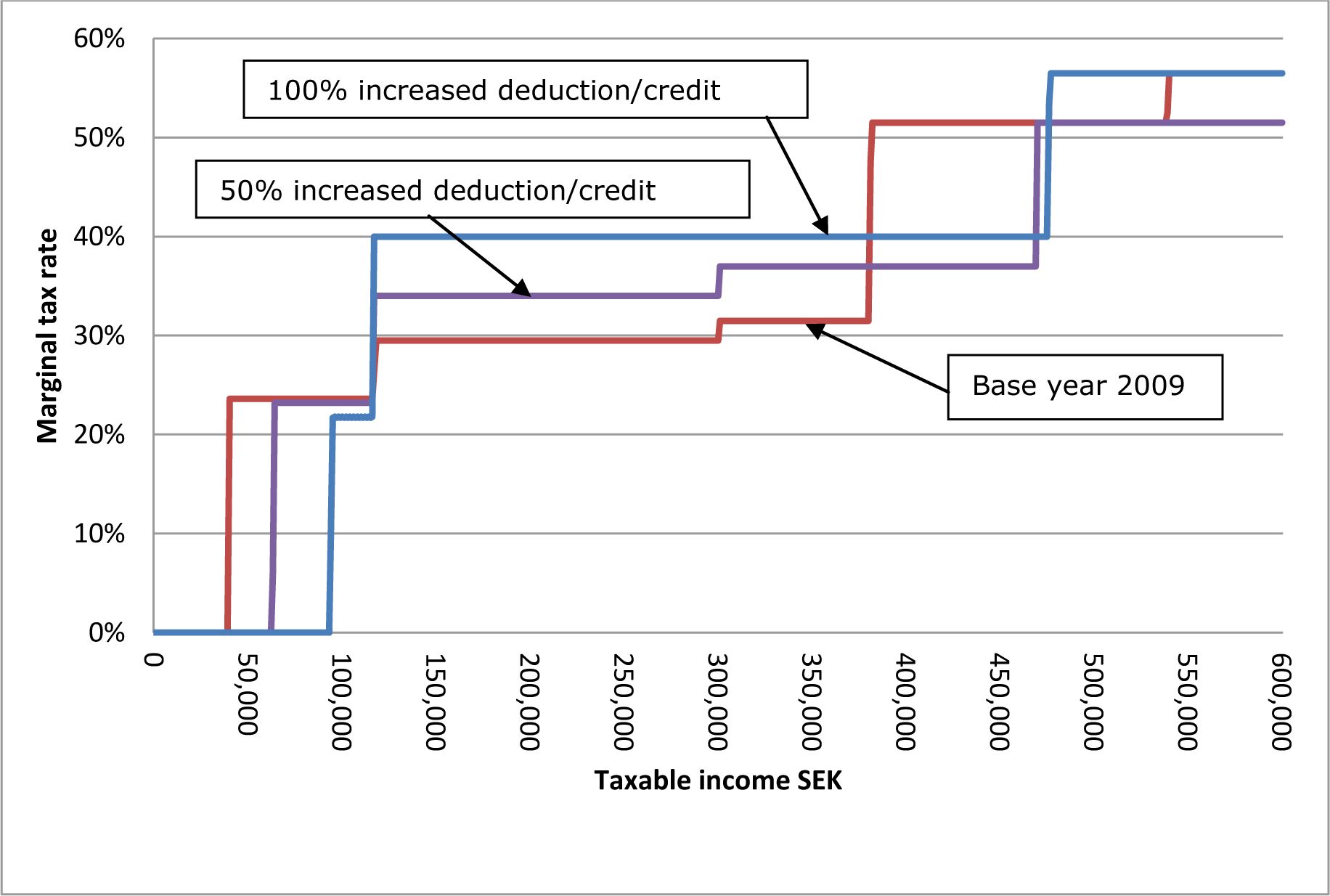
The two profiles compared to the base year 2009 are presented in Figure 3.
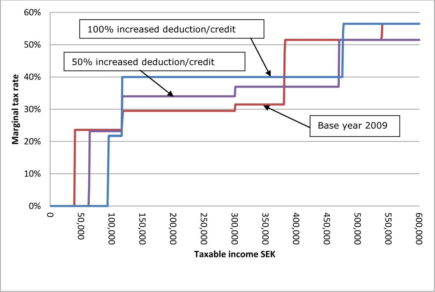
The optimal tax profiles compared to the base year 2009.
A natural criticism of these profiles is that most income earners obtain a higher marginal tax compared to the level in 2009. As mentioned above, this is caused by the large increase in deduction/credit, and hence the alternative design with a smaller increase (50 percent) seems appealing. This produces a profile that is much more like the 2009 design, but compared to 2009 the alternative design benefits low-income earners due to the higher basic deduction, while at the same time high-income earners benefit from a lower marginal tax rate. The lower increase in the credit/deduction also benefits median-income earners due to a lower compensatory tax increase. The increased basic deduction gives a lower average tax rate for both low and median incomes.
Given this background, there seem to be reasons to pick reform 78 as the optimal design. Lower national taxes, increased credit/deduction, and increased housing allowances are balanced to achieve efficiency and equity and to benefit individuals who before the reform had the lowest welfare.
Finally, it is interesting to compare the welfare levels of the budget neutral variants of the flat and age dependent taxes in Table 4 and 5 above. A flat tax of 29.5 percent is budget neutral and implies a large increase in hours of work and hence also in labour income and disposable income. However, due to the large increase in income inequality, an increase in Gini by 10 percent, the welfare ranking is low. in fact, according to W1 -W3 the reform is amongst the lowest of all designs and according to W∞ the rank is number 17. The age dependent neutral tax has a phase in and out rate of 1.85 and this reform has similar welfare ranking as the neutral flat tax for W1 -W3 and lower according to W∞. The large increase in income inequality of these two designs has a heavy impact on the welfare measures.
8. Summary and conclusion
Among the large number of tax/benefit designs included in this evaluation, a few clear results appear. Tax/benefits compatible with high social welfare should not produce large marginal effective tax rates or a too large dispersion in welfare17. The importance of income inequality in the evaluation of welfare is illustrated by comparing two benefits such as child and housing allowance. An increased housing allowance, targeting low-income households, has a much larger effect on welfare than an increased child allowance. The importance of reduced marginal effective tax rates follows from the observation that a decreased national tax is a common feature of the tax designs with highest welfare. Even dropping the highest national tax can be defended based on the welfare argument. The importance of the in-work tax credit deserves to be mentioned for its double merits: reduced replacement rates lead to increased employment, which reduces the income inequality.
Based on the analysis results, an optimal tax design with the 2006 tax rules as a reference could be formulated as follows: to create incentives for income from work instead of benefits and to utilize that an increased number of working hours for high-income earners generates large tax revenues, a combination of an increased basic deduction and in-work tax credit and reduced national taxes is proposed. Social welfare is increased if pensioners as well as individuals on sickness disability and the unemployed receive a higher basic deduction. There are no arguments for increasing the child allowance since it does not target low-income families. The housing allowance should be increased since it targets households with low welfare and also comes at a low budgetary expense. The reform should be financed by a tax increase based on the same tax base as the municipal income tax.
For this kind of evaluation, it is important to state the underlying assumptions. This is a study of how households change income and working hours due to changes in taxes and benefit systems. It is important to realize that the study of behavioral changes is based on a partial approach, i.e., only the supply of labour is considered and not the demand. our analysis assumes a certain degree of adaption and a positive demand for workers. However, it should be remembered that the estimated parameters that are included in the models for labour supply and participation are affected by the labour market conditions during the period of estimation. A more balanced view regarding the criticism due to absence of a demand side is that we assume a labour market similar to the situation during the period used for estimation of the statistical models.
The behavioural models included do not produce strong responses to changed economic incentives. If there is any systematic bias, it is more probable that these effects are underestimated. Although the whole population is included in the evaluation, not all working-age individuals are allowed to change working hours, for instance students and older children who are living with their parents. Modelling mobility between studies and work and the importance of economic incentives in this process is complicated, and it is not obvious how to do this in static models. Including older children in the analyses requires household models with more than two adults, and we are not aware of any such study. At the same time, it should be mentioned that our analysis has an unusually broad coverage, the whole population is included and most individuals aged between 16 and 70 are allowed to change their labour supply. A related problem is that we only consider different working states on a full-year basis, i.e., disability whole year, unemployed whole year, etc. Thus, a rather large change in the replacement rate is required in order to change between different full time statuses. In principle it is possible to develop a future version of the model that can handle part-time status and presumably also students and older children. However, the fact that this is not part of the current model is an argument against overestimation of the impact of economic incentives.
To continue the discussion of assumptions and simplifications in this kind of analysis, the focus on an optimal tax on labour income is a simplification since the whole tax mix should be analyzed. For instance, one argument in favor of a flat tax is that it creates possibilities to minimize the problem caused by different tax rates on income from capital, corporate taxes, and labour. The administrative costs linked to corporate taxation are one reason why the OECD considers a corporate tax reform as a high priority issue. This is a topic not at all considered in this analysis.
Another potential criticism is the focus on welfare criteria in the evaluation of tax/benefit reforms. An ageing population has increased the awareness of the need for high tax revenues for many years to come. If this problem is taken seriously, then the focus should be on reforms that maximize tax revenues or minimize government net expenditure. A focus on working hours instead of welfare is again an argument for a flat tax design.
One crucial issue not included explicitly in this paper is the question of short- or long-run effects. This is a static analysis and the standard interpretation is that we only consider changes in a market in equilibrium. That is, we do not study how individuals adapt to a change but rather how they behave after they have adapted, i.e., long-run effects. Another approach to study the long-run effects would be to study the change over the whole life cycle. A reform can have different effects depending on the age of the individual and these effects can last for many years. A life cycle perspective can give different conclusions regarding an optimal design compared to our static analysis.
In a long-run perspective, reforms that have a large effect on labour supply will have a different assessment compared to our static approach. A 25 percent flat tax and a simulated four percent increase in working hours would at a 20–30 year horizon produce dramatically higher economic growth compared to the alternative designs that in our analysis produced the highest welfare. However, the increase in income inequality and the potential risk of reduced tax revenues of a low flat tax should also be mentioned.
Footnotes
1.
For practical reasons, income tax is used synonymously with tax on earnings; taxes on capital are not included in this analysis.
2.
See, e.g., Mirrlees (1971), Stern (1976), and for a review Tuomala (1990).
3.
For a survey of static microsimulation models in Europe, see Sutherland (1995).
4
The definition used for welfare participation is that the household received social assistance.
5.
For a description of LINDA, see Edin & Fredriksson (2000).
6.
Group size as a sample percentage: (1) 27.3, (2) 10.1, (3) 7.4, (4) 2.6, (5) 1.3, (6) 2.6, (7) 3.5, (8) 1.3 and (9) 43.9.
7.
Of course in practice the tax/benefit module is evaluated 7 times for singles and 49 for spouses and each time disposable income with and without social assistance is calculated. The different means of the intervals used to approximate the distribution of working hours are: 0, 500, 1,000, 1,500, 2,000, 2,500, and 3,000 (hours worked per year).
8.
For a detailed presentation of all models including the estimated parameters, see Ericson, Flood, and Wahlberg (2009).
9.
An alternative to the traditional model used here is the collective approach. This approach takes into account the fact that the household members may have different preferences. Among these household members, an intrahousehold bargaining process is assumed to take place. For a review see Vermeulen (2002).
10.
What may appear as “stigma" or disutility from welfare participation may also result from errors in measuring true welfare eligibility. Moreover, imperfect information regarding benefit eligibility on behalf of the household is also included in this non-monetary cost.
11.
This section is largely based on Aaberge and Flood (2008) and Aaberge and colombino (2008). For details we refer to these sources.
12.
There is of course a problem of selecting the correct equivalence scale. A simple sensitivity test has been performed where we found that different choices of scaling factors produced similar parameters. However, whether these choices produce a different welfare ranking of tax/benefit designs have not been tested.
13.
The table of the results is not included but is available from the authors upon request.
14.
Note, the national tax is defined as the 20 percent tax above the first breaking point and the highest national tax is defined as an additional 5 percent tax above the second breaking point.
15.
Note that of all the results reported in the table it is only the welfare measures that are subject to budget neutrality.
16.
Alternatively, the effects of the reforms could have been evaluated conditional on budget neutrality. However, given the large amount of information already included we decided to not include this evaluation.
17.
Marginal effective tax rates refer to the combined effects of taxes and transfer programs.
References
-
1
Characterizations of Lorenz Curves and Income DistributionsSocial Choice and Welfare 17:639–653.
-
2
Axiomatic Characterization of the Gini Coefficient and Lorenz Curve OrderingsJournal of Economic Theory 101:115–132.
-
3
Designing Optimal Taxes with a Microeconometric Model of Household Labour SupplyScandinavian Journal of Economics (forthcoming).
-
4
Evaluation of an In-Work Tax Credit Reform in Sweden: Effects on Labor Supply and Welfare Participation of Single MothersIZA DP, No. 3736.
-
5
The Base for Direct TaxationIn: J Mirrlees, S Adam, T Besley, R Blundell, S Bond, R Chote, M Gammie, P Johnson, G Myles, J Poterba, editors. Chapter 6 in Dimensions of Tax Design: the Mirrlees Review. Oxford University Press. pp. 548–674.
-
6
Employment, Hours of Work and the optimal Taxation of Low Income FamiliesReview of Economic Studies (forthcoming).
-
7
Microsimulation as a Tool for Evaluating Redistribution PoliciesJournal of Economic inequality 4:77–106.
-
8
Means testing and tax rates on earningsIn: J Mirrlees, S Adam, T Besley, R Blundell, S Bond, R Chote, M Gammie, P Johnson, G Myles, J Poterba, editors. Chapter 2 in Dimensions of Tax Design: the Mirrlees Review. Oxford University Press. pp. 90–201.
-
9
LINDA – Longitudinal individual DAta for Sweden. Working Paper 2000:19Uppsala Universitet, Nationalekonomiska institutionen.
-
10
SWEtaxben: A Swedish Tax/benefit Micro Simulation Model and an Evaluation of a Swedish Tax Reform. Working paper No 346 in S-WOPECSWEtaxben: A Swedish Tax/benefit Micro Simulation Model and an Evaluation of a Swedish Tax Reform. Working paper No 346 in S-WOPEC, http://swopec.hhs.se/gunwpe/abs/gunwpe0346.htm.
-
11
Svensk finanspolitik Finanspolitiska rådets rapport 2008Svensk finanspolitik Finanspolitiska rådets rapport 2008, http://www.finanspolitiskaradet.se/download/18.cd1771b11927f1f0c6800085452/Svensk+fina nspolitik+2008.pdf.
-
12
Household Labor Supply and Welfare Participation in SwedenJournal of Human Resources 39:1008–1032.
-
13
From Welfare to Work: Evaluating a Proposed Tax and Benefit Reform Targeted at Single Mothers in SwedenLABOUR 21:443–471.
-
14
The Elasticity of Taxable Income: Evidence and ImplicationsJournal of Public Economics 84:1–32.
- 15
-
16
Welfare Reforms in European Countries: A Microsimulation AnalysisEconomic Journal 117:1–44.
- 17
-
18
An Exploration in the Theory of Optimal Income Taxation175–208, Review of Economic Studies, 38, 31.
-
19
http://www.oecd.org/ctp/taxingwagesTaxing Wages 2006–2007 Special feature: Tax reforms and tax burdens.
-
20
http://www.oecd.org/economics/goingforgrowthEconomic Policy Reforms: Going for Growth.
-
21
Fundamental Tax Reform: The Experience of OECD Countries. Background Paper Number 47Tax Foundation.
- 22
-
23
Using Elasticities to Derive Optimal Income Tax RatesReview of Economic Studies 68:205–229.
-
24
Optimal Income Transfer Programs: Intensive versus Extensive Labour Supply ResponsesQuarterly Journal of Economics 117:1039–1073.
-
25
Optimal Taxation and Optimal Tax SystemsJournal of Economic Perspectives, American Economic Association 4:157–78.
-
26
On the specification of models of optimal income taxationJournal of Public Economics 6:123–62.
-
27
Static Micro-simulation Models in Europe: A survey. DAE Working Paper No 9523University of Cambridge.
- 28
- 29
-
30
Collective Households Models: Principles and Main ResultsJournal of Economic Surveys 16:533–564.
-
31
The Surprising Power of Age-Dependent Taxes. Working Paper 11–114Harvard Business School.
- 32
-
33
Simple solutions to the initial conditions problem in dynamic, nonlinear panel data models with unobserved heterogeneityJournal of Applied Econometrics 20:39–54.
Article and author information
Author details
Acknowledgements
Financial support from the Jan Wallander and Tom Hedelius Foundation for Research in Economics, the Confederation of Swedish Enterprise, Riksbankens Jubileumsfond and Ragnar Söderbergs stiftelse is gratefully acknowledged. We would also like to express our gratitude to Rolf Aaberge for his support and constructive criticism.
Publication history
- Version of Record published: December 31, 2012 (version 1)
Copyright
© 2012, Ericson and Flood
This article is distributed under the terms of the Creative Commons Attribution License, which permits unrestricted use and redistribution provided that the original author and source are credited.