On weights in dynamic-ageing microsimulation models
- Federal Planning Bureau, Belgium
- CESO, Katholieke Universiteit Leuven, Belgium
- CEPS/INSTEAD, Luxembourg
- Australian National University, Australia
Abstract
A dynamic model with cross-sectional dynamic ageing builds up complete synthetic life histories for each individual, starting from a survey dataset or an administrative dataset. Many of these datasets include weights. This is a problem for dynamic microsimulation models, since the most obvious solution, expanding the dataset, is not always advisable or even possible. This short paper presents an alternative method to use weights in dynamic microsimulation models with dynamic ageing. This approach treats the weighting variable as just another variable in the model, and the weights are only used after simulation to derive weighted simulation results. Tests using Australian data confirm that weighted variables give sensible results, with reductions in runtimes and memory requirements.
1. Introduction
Dynamic models with cross-sectional dynamic ageing build up complete synthetic life histories for each individual in the dataset, including data on mortality, labour market status, retirement age, savings and so on (Emmerson, et al., 2004, 3). They do so starting from a survey dataset or an administrative dataset. Many of these datasets include weights, which are needed so that the sample reflects unbiased and credible sample estimators of population parameters. This is a problem for dynamic microsimulation models, since the most obvious solution, expanding the dataset, is not always advisable or even possible with unscaled probability weights or frequency weights.
This short paper presents an alternative method, using weights in dynamic microsimulation models, rather than simply expanding the dataset. The paper starts by briefly discussing the use of weights. As expanding the starting dataset using the frequency weights is in many cases not a feasible option, an alternative way of using weights will be presented. This approach treats the weighting variable as just another variable in the model, and the weights are only used after simulation to derive weighted simulation results. The consequences of using weights in the case of alignment are discussed. Tests using Australian data confirm that weighted variables give sensible results, with reductions in runtimes and memory requirements. Runtime and memory reductions may be particularly useful for short time span projections. The first author developed the concepts and theoretical analysis, and the second author did the testing. The authors have not been able to find any references to dynamic microsimulation models using weights
2. Using weighted data in microsimulations
2.1 Why weights?
National statistical agencies often carry out household surveys, assigning weights to each respondent household. For example, the Australian Bureau of Statistics (2003a, 7) surveyed incomes and housing costs, using sampling rates dependent on state or territory. Panel data sets also often use household weights, which need to change as households cease responding, new households are added and overall population characteristics change. Census sample files, such as the 1% sample file available from the Australian 2001 census, may have known biases which can be approximately corrected using weights. If complete administrative records are not available as a starting point for cross-sectional dynamic models, it may be necessary to use weighted data.
2.2 Using frequency weights to expand datasets before simulation
A straightforward way of using frequency weights is to ‘expand’ the starting dataset before simulation. Frequency weights are integer numbers that represent the number of population cases that each sample case represents. When each object (household or individual) has a frequency weight fx, then the population can be derived from the sample by replacing each object by fx copies of itself. Put differently, fx-1 clones are made of each object with weight fx. The starting dataset thus ‘absorbs’ the weights and becomes the population, and the model can be run as would be the case without weights. This data expansion however can be a problem since dynamic-ageing microsimulation models already use a lot of memory, and require a lot of time to run. Expanding the starting dataset obviously enhances these problems.
2.3 Using weighted data during simulations
This paper presents an alternative way in which frequency weights can be included in dynamic microsimulation models. In contrast to the previous approach, the weights are not used to expand the starting dataset before, but are used and modified during simulation. So the previous approach used the weights to change the starting dataset of the model, and then applied the model to this dataset. Now we do not change the starting dataset, but treat the household weight variable as any other variable. The simulated weights are then used to weight the simulated dataset in the production of aggregates, indices of poverty and inequality, et cetera. The discussion will pertain to household weights, but the situation in case of individual weights will be an obvious simpler case.
2.4 Simulation of events involving only one household
The weighting variables in most survey datasets are ‘shared weights’ that pertain to the household level. This is all the more important in the case of microsimulation models, since weighting needs to preserve the household structure, because this structure is later needed to simulate equivalent household income that forms the basis of indicators of poverty and inequality. However, when individuals share an equal weight when they are members of the same household, then this has consequences when new individuals or households appear during simulation. To see this, remember that a frequency weight equal to 10 implies that an observed individual represents 10 ‘actual’ individuals with the same characteristics. When a new individual appears through birth, then the obvious solution is that the newborn receives the same weight as the other members in the household. So in our example, it is as if 10 households each received a newborn child. An equally obvious situation appears when someone leaves a household to start a one-person household of his or her own. This can be the case when a child ‘leaves the nest’, or when a couple divorces. In this case, the result is two households with equal weight. A third and final example of an obvious situation is when a household immigrates or emigrates. In this case, it is as if 10 households entered or left the country.
2.5 Simulation of events involving more than one household
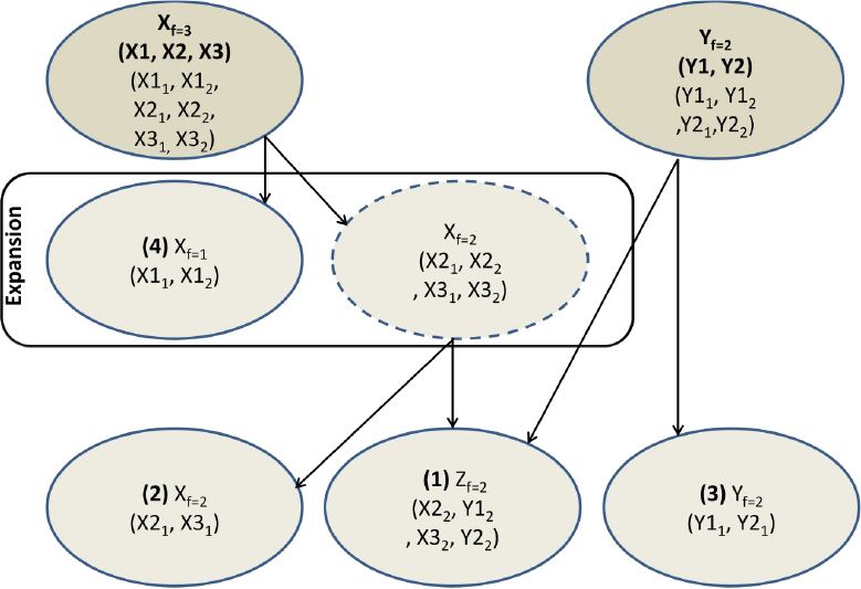
A more complicated situation however arises when two individuals from different households with different weights form a third household. What weight should this newly created household get? To see the problem more clearly, suppose two households X and Y. Both households consist of two individuals, denoted X1, X2, Y1 and Y2. Now suppose that individuals X2 and Y2 fall in love and form a new household, say, Z. What frequency weight should this household get?
Start from the obvious case where the frequencies of both households are equal, say fx = fy = 3. In this case, the frequency weight of the new household is also equal to 3. Or, one individual X2 from three households 2 and 3 of type X (X22 and X32) forms a partnership with one individual Y2 from three households 1 and 2 of type Y (Y12 and Y22), hence creating three new households of type Z. The case where the weight of both donating households is exactly the same is however trivial in that it will seldom appear.
Suppose next that the frequencies of both households is fx = 3 and fy = 2. The problem arises from the fact that the weights fx and fy are unequal. This situation is described in Figure 1. The solution again lies in interpreting it as if the dataset was expanded: there are 3 households of ‘type x’ and 2 households of ‘type y’. Denote these expanded households X1 to X3 and Y1 and Y2. Hence, individual Y2 of both households Y1 and Y2 forms a partnership with individual X2 from two out of three households X. The result is that there are two new households Z1 and Z2, both consisting of a pair of individuals X2 and Y2. There are also two ‘old’ households Y, of which individual Y2 has left, and only Y1 remains. Likewise, there are two ‘old’ households X, of which individual X2 has left, and only X1 remains. Finally, one household of type X remains unchanged, consisting of X2 and X1. In short, when the frequency weights of the two ‘donating’ households differ, the household with the highest frequency (in this case household X with fx = 3) is expanded to two households, of which one has a weight equal to fy.

Example of the alternative strategy.
2.6 General formulation
More generally, the problem is as follows. Donating households X and Y consists of nx and ny individuals (nx, ny≥1) and have frequency weights fx and fy (fx, fy≥1, fx≠fy). Summarize these households as X[x1..xnx; fx] and Y[y1..yny; fy]. Individuals x1 and y1 from the donating households form a new household Z with an unknown frequency weight fz. The solution is to break up X and Y to subsets with equal weights fz = min(fx, fy), and then create Z with weight fz. The resulting situation is
Household Z[x1, y1; fz] is the new created household.
Household X[x2..xnx; fz] is the donating household X without individual x1.
Household Y[y2..ynx; fz] is the donating household Y without individual y1.
Household X[x1..xnx; fx − fz] is the remaining donating household X with individual x1.
Household Y[y1..ynx; fy − fz] is the remaining donating household Y with individual y1.
Note that either cases 4 or 5 are empty.
In the previous example, nx = ny = 2, fx = 3 and fz = 2. The solution then is
Household Z[x1, y1; 2] is the new created household with frequency weight 2.
Household X[x2; 2] is the donating household X without individual x1.
Household Y[y2; 2] is the donating household Y without individual y1.
Household X[x1,x2; 1] is the remaining donating household X with individual x1.
Household Y[y1..y2; 0] is the remaining donating household Y with individual y1. This household does not exist in the solution.
Where the numbers 1 to 4 are shown in Figure 1.
2.7 Gradual decrease in weights
The method presented in this paper involves the partial expansion or “splitting up” of individual weighted households in case of moves of individuals in between households of different weights. As a result of a continuous process of moves and the accompanying partial expansions, the average size of the weights will gradually decrease as the dataset becomes more and more expanded. In some future simulation year, all weights will have been reduced to one, and the dataset will have been fully expanded.
3. Alignment and weights
The alternative strategy of treating the frequency weight as any other variable has as the main advantage that it prevents large losses in efficiency involved in expanding the starting dataset. However, a problem arises in how the microsimulation model applies alignment procedures. Alignment is a general name for a set of procedures for achieving an aggregate simulation result in line with a desired result, usually based on predictions of semi-aggregate models or social-policy scenarios. If ‘aggregate simulation result’ is defined as an average or sum of a continuous variable (usually earnings or income) then the procedure is known as ‘monetary alignment’. If the ‘aggregate simulation result’ is the number of persons in a state or experiencing an event, we discuss ‘state’ or ‘event alignment’ of discrete variables.
If the starting dataset is expanded to take into account frequency weights, then all alignment procedures should be unaffected. If weights are treated as any other simulation variable, as is the case in our alternative strategy, then applying alignment without taking them into account will result in simulation errors. The simulation results need to equal the exogenous data after the weights have been applied. The procedures used to align models based on weighted data will depend on the situation, being strongly affected by the alignment precision and runtime reductions required.
In theory, alignment totals for persons in each possible state can be replaced by alignment totals for each possible event leading to that state. In practice, calculating the event alignment totals may be difficult, as the sources for the state alignment totals are likely to lack the necessary detail. For this paper, however, we assume that state alignment can be achieved by event alignment.
Li and O’Donoghue (2011) provided distortion and computational cost measures for seven different event alignment methods. They concluded that “selecting the ‘best’ alignment method is not only about the algorithm design, but also the requirements and reasoning in a particular scenario”. The last three of the methods they tested involved sorting the records according to some calculated rank, and selecting cases in rank order until the desired alignment total was reached. Of these three “alignment by sorting” methods, SBDL (sorting by the difference between logistic adjusted predicted probability and random number) has been widely used since its suggestion by Johnson (Morrison 2006).
Cumpston (2009) suggested an “alignment by random selection” method, involving randomly selecting cases for event simulation until the event alignment total was reached. He showed that its distortion performance was similar to that of SBDL.
3.1 Event alignment with weighted records
Alignment by random selection, as well as by sorting, can readily be used with weighted records, as each involves selecting cases until the desired alignment total is reached. The only new problem is that the weight of the last selected case may cause the simulated total to exceed the alignment total. We suggest three strategies to deal with this problem, and provide test results using the first and third of these strategies.
3.1.1 Strategy 1: split up the last household.
Suppose the last selected household has caused an overshoot beyond the alignment total. Then that household can be split into two parts, one simulated to have enough events to reach the alignment total, and the other simulated not to have any events.
3.1.2 Strategy 2: select a household for alignment to give the lowest possible mismatch
When the last selected household has caused an overshoot beyond the alignment total, discard that selection, and continue selecting households until an exact match is obtained. If no exact match can be obtained, select the household giving the minimum mismatch. If using sorting by random selection, a limit should be placed on the total number of selections after overshoot.
3.1.3 Strategy 3: carry forward any misalignment to the next period
Here the best alternative is chosen between implementing the event for the whole or none of the last household, depending on which alternative results in the smallest mismatch. In case the last household is chosen not to have the event, the resulting shortfall in event numbers is added to the alignment total for the next period. In the alternative case, there is an excess in event numbers, which is then deducted from the alignment total of the next period.
3.2 What are the advantages and disadvantages of these strategies?
The first strategy requires the least possible number of selections, but requires further splitting up of weighted households, thereby reducing the marginal efficiency gain of weighting the dataset.
The second strategy avoids splitting up households, but has two disadvantages. Many more records may have to be selected, and the degree of mismatch is not controlled.
The third strategy requires no additional splitting, and no additional selections have to be made. Differences from alignment targets should largely cancel each other out over several periods.
3.3 Australian data used for testing
Weighted unit records from the 2000–01 Survey of Income and Housing Costs (SIHC), Australian Bureau of Statistics (2003a), were converted into suitable input files for this model. These files covered 16,824 persons, grouped into 6,786 households.
Dwelling weights in the SIHC sample were intended to replicate the Australian population of about 19.4m. To give an unweighted sample size of about 175,000, the weights were multiplied by 0.00937, obtaining dwelling weights ranging from 1.66 to about 34. These weights were then rounded to the nearer integer. For these tests, the sample data were split into 8 regions (the seven states and the Australian Capital Territory), and migration modelled between the regions.
3.4 Model changes to use weighted data
The SIHC dataset was run with the Cumpston model (2009). The model was extended to input, store and update a weight for each occupied and vacant dwelling. A particularity of this model is that it simulates dwellings separately from households. When a household moves out of a dwelling, the dwelling is assumed to continue in existence as a vacant dwelling, with the same location, structure, market value and potential rent. Then the destination for a moving household is simulated, taking into account the destination patterns of moving households. Finally, out of three randomly-selected vacant dwellings, the one most closely meeting the housing patterns of the moving household is chosen. For the purpose of this paper, this procedure was adapted to incorporate weights as follows:
if the weight of the moving household is greater than the weight of the selected dwelling, that dwelling is assumed to be become fully occupied, and the weight of the source household is reduced accordingly, with destination and dwelling searching by the source household continuing
if the weights are equal, the source household occupies the selected dwelling, with the source dwelling becoming vacant, and keeping its original weight
if the weight of the moving household is less than the weight of the selected dwelling, the selected dwelling is assumed to become occupied with weight equal to that of the source dwelling, and an identical vacant dwelling is assumed in the destination area, with weight equal to the difference between the selected and source dwellings.
Similar principles were used for exits (where an exit is any move of one or more persons out of a dwelling, where at least one person remains in the dwelling), and immigrants. The microsimulation model contained assumptions about the numbers of immigrants each year, and their destination, age and type distributions. The same immigration assumptions were made, with each immigrant household given a weight of 10 (chosen to be close to the average weight of 10.4 for dwellings at the start of each microsimulation).
Thus, the separate modelling and simulation of households and dwellings introduces additional splitting of households in the simulation process, on top of the splitting required for marriage, cohabitation, and the alignment processes.
3.5 Alignment methods used during testing
Alignment totals for births, deaths, emigrants and immigrants were available for 8 regions, subdivided into 9 age-groups. Alignment by random selection was used to give one-pass alignment of these events for each combination of region and age-group. Alignment was thus done separately for each of 72 alignment pools, for each of four event types. To allow random sampling within each alignment pool, lists of person reference numbers were maintained for each pool, updated each time a person changed regions, and recreated each year to allow for age changes.
For example, the alignment total for deaths amongst persons aged 75 to 84 in Victoria in the third projection year was 105. Persons were selected at random from those in this alignment pool, and if their probability of death was greater than a random number between 0 and 1, assumed to die. The number of deaths for the pool was increased by the weight for the household, unless this would have given total deaths exceeding 105. Applying the first alignment method, a death resulting in an excess over the alignment total was dealt with by splitting the household, so that enough persons died to exactly reach the total, and the remainder were assumed to remain alive. For example, if 100 persons had already been simulated to die, and the next person simulated to die had a household weight of 15, then 5 persons would be assumed to die, and the remaining 10 remain alive in a new household. Death simulation for the pool ceased when the alignment total was reached.
This alignment process created some additional household splitting, on top of the splitting due to the process of marriage, cohabitation and household moves. This reduced the performance gains potentially available from the use of weights. As an alternative, the third proposed alignment method was therefore tested, choosing the best alternative between implementing the event for the whole or none of the last household, and carrying forward any misalignments to the next period. In the above example, assuming all the persons to die in the last household would have exceeded the alignment total by 10, while assuming none to die would have fallen short by 5. No persons would thus have been assumed to die in the last household, and the alignment total for the next period would have been increased by 5. This modified alignment strategy was used in the cases with alignment in tables 1 and 2.
50-year projections using unweighted and weighted data.
| Weighted Data | Alignment | Moves | Runtime (seconds) | Runtime as % of unweighted | Average number of records as % of unweighted |
|---|---|---|---|---|---|
| No | No | Yes | 39.07 | 100.0% | 100.0% |
| Yes | No | Yes | 31.35 | 80.2% | 81.6% |
| Yes | Strategy 1 | Yes | 32.60 | 83.4% | 83.0% |
| Yes | Strategy 3 | Yes | 32.49 | 83.2% | 82.3% |
| No | No | No | 31.58 | 100.0% | 100.0% |
| Yes | No | No | 19.72 | 62.4% | 57.9% |
| Yes | Strategy 1 | No | 20.52 | 65.0% | 60.5% |
| Yes | Strategy 3 | No | 20.12 | 63.7% | 58.5% |
3.6 Tests using Australian data
The SIHC dataset was run with the Cumpston model (2009), using birth, death, emigration and immigration assumptions chosen so as to give a 2051 population estimate approximately equal to the 34.2m projected by the Australian Bureau of Statistics (2008, 39, series B).
Alignment was based on national population projections (Australian Bureau of Statistics, 2003b), providing yearly projections of births, deaths, emigrants and immigrants for each region, and subdivisions of these event numbers were obtained for 9 age-groups (0–14, 15–24, 2534, 35–44, 45–54, 55–64, 65–74, 75–84, 85+). More recent population projections (Australian Bureau of Statistics 2008) showed higher growth, so the alignment totals were multiplied by 1.383 for births, 1.006 for deaths, 1.077 for emigrants and 1.275 for immigrants. These subdivided numbers were used as alignment totals, for the tests with event alignment. No alignment totals were available for household exits or household moves.
For the weighted data, the numbers of immigrant families in each year were too low to properly reflect the diversity of immigrants, so immigrant families for each projection decade were pregenerated at the start of the decade, and randomly drawn without replacement. Close alignment was obtained each year for births, deaths and emigrants, but alignment of immigrants occurred over each decade.
3.7 Results of tests using Australian data
The first line of Table 1 describes the results when the weighting procedure is not applied and the model is run on the ‘expanded’ dataset. Averaging over 10 runs, the average runtime between 2001 and 2051 was 39.07 seconds. The second line shows that applying the weights method proposed in this paper reduced the average runtime by about 20% to 31.35 seconds. The average number of person records during the 50 years was about 81.6% of the number with unweighted data. A “person record” is the record of all the details for an individual, including the weight of the household in which the person lives. For this example, the number of person records at the start of the 50 years was 9.6% of the number with unweighted data, rising to 99.4% at the end of the 50 years. The 80.2% runtime as a percentage of the unweighted runtime is broadly similar to the 81.6% average number of records as a percentage of the unweighted records, as most of the simulation calculations are per record.
Line 3 of Table 1 shows that using alignment strategy 1 increased the runtime from 80.2% to 83.4% of the unweighted runtime. This is partly due to the additional record splitting caused by alignment strategy 1, as shown by the increase in the average number of records, as a percentage of the unweighted case, from 81.6% to 83.0%. Line 4 of Table 1 shows that using alignment strategy 3 gave slightly lower runtimes, and slightly fewer records, than strategy 1. These results were as expected, as strategy 3 selects the best alternative between implementing the event for the whole or none of the last household, depending on which alternative results in the smallest mismatch. strategy 1 exactly achieved the alignment targets for births, deaths and emigrants, and strategy 3 very closely achieved the targets.
Lines 5 to 8 of Table 1 are similar to lines 1 to 4, except that no household moves are assumed (a common assumption in models with only one region). Using weighted data with no alignment reduced the average runtime by about 38%, compared with the 20% saving with household moves simulated. Alignment strategy 1 again gave modest increases in runtimes and record numbers, with strategy 3 giving slightly lower increases.
4. Convergence from weighted to unweighted projections
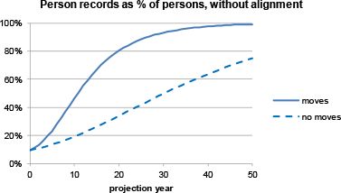
The method presented in this paper involves the partial expansion or “splitting up” of individual weighted households in case of moves of individuals in between households of different weights, or of households in between dwellings. As a result of a continuous process of moves and the accompanying partial expansions, the average size of the weights will gradually decrease as the dataset becomes more and more expanded. In some future simulation year, all weights will have been reduced to one, and the dataset will have been fully expanded. The total efficiency gain of using weights in the way suggested by this paper depends on the average initial size of the weight, and the speed of the convergence process. This is illustrated in Figure 2.

Weighted and unweighted person projections.
As a benchmark, the number of person records of the unweighted (fully expanded) dataset is for all projection years set to 100%. The difference between the curve and the 100% line thus shows the ‘relative expansion’ of the weighted dataset at any moment in time. Figure 2 shows that the numbers of weighted person recorded, in the unrestricted projections using weighted SIHC data, rose quickly, and after 50 years were about 99% of the unweighted numbers. Clearly, the efficiency gain that comes with the approach proposed in this paper is achieved in the first part of the simulation period. The more splitting up is required, the faster the marginal efficiency gain is reduced. The bottom line in Figure 2 reflects the development of the number of person records when moves of households between dwellings are not simulated, and additional splitting is thus avoided. In this case, expansion takes place at a lower rate and the efficiency gain pertaining to using weights is therefore larger.
5. Conclusions
This short paper discusses the use of weights in dynamic microsimulation models with dynamic ageing, other than simply expanding the dataset. An alternative approach is presented, that treats the frequency weights as just another variable in the model. These weights are then used during simulation to derive weighted simulation results. This alternative strategy can give savings in runtimes and memory requirements, with the size of the savings depending on the circumstances.
Tests using Australian data showed that microsimulations using weighted data, or unweighted data derived from weighted data, can give reasonable total population projections. With these test data, runtimes for microsimulations using weighted data are reduced by about 20% if moves of whole households are simulated, and by 38% if such moves are not simulated. The marginal efficiency gain however decreases with the increase of the simulation period, and this reduction pertains to the amount of splitting required. The efficiency gain is therefore limited to the first few decades.
Finally, the consequences of using weights in the case of alignment are discussed. This paper proposes three ways in which alignment can take weights into account, and gives test results with two of these methods. using either of the two strategies tested gave good alignment with marginal increases in runtimes.
Efficiency and memory gains may be quickly lost due to (a) “splitting” in a complex environment (a simulation with many different events happening), (b) a long duration simulation, (c) a simulation in which there is detailed, disaggregated alignment or (d) a combination of the above.
Footnotes
1.
The ideas in this paper were previously presented at the Ministero dell’Economia e delle Finanze, dipartimento di Tesoro, Rome, Italy, February 14th, 2011, and the 3rd General Conference of the International Microsimulation Association,”Microsimulation and Policy Design” June 8th to 10th, 2011, Stockholm, Sweden. The authors are grateful for the comments by the participants in these meetings. Thanks also to two anonymous reviewers and to Robert Tanton for assuming the role of editor for this paper.
References
-
1
Survey of income and housing costs Australia 2000–01 – confidentialised unit record file (CURF) technical paperSurvey of income and housing costs Australia 2000–01 – confidentialised unit record file (CURF) technical paper, catalog no, 3222.0, Canberra August, 63 pages.
-
2
Population projections Australia 2002–2101Population projections Australia 2002–2101, catalog no 3222.0, Canberra September 3, 186 pages.
-
3
Population projections Australia 2002–2101Population projections Australia 2002–2101, catalog no 3222.0, Canberra September 3, 96 pages.
-
4
Acceleration, alignment and matching in multi-purpose household microsimulationspaper presented during the Second General Conference of the International Microsimulation Association, Ottawa, June 8–10, 22 pages, available from, http://www.microsimulation.org/IMA/ottawa_2009.htm.
-
5
Life Cycle Microsimulation ModellingWhat are the consequences of the European AWG-projections on the adequacy of pensions? An application of the dynamic micro simulation model MIDAS for Belgium, Germany and Italy, Life Cycle Microsimulation Modelling, Lambert Academic Press.
-
6
On weights in dynamic-ageing microsimulation modelspaper presented during the 3rd General Conference of the International Microsimulation Association: “Microsimulation and Policy design”, Statistics Sweden, Stockholm, Sweden, June 8th to 10th, available on, http://www.scb.se/Grupp/Produkter_Tjanster/Kurser/_Dokument/IMA/Dekkers_cumpston.pdf.
-
7
An Assessment of PENSIM2, IFS Working Paper WP04/21London: Institute for Fiscal Studies.
-
8
Evaluating alignment methods in dynamic microsimulation modelspaper presented during the 3rd General Conference of the International Microsimulation Association: “Microsimulation and Policy design”, Statistics Sweden, Stockholm, Sweden, June 8th to 10th available on, http://www.scb.se/Grupp/Produkter_Tjanster/Kurser/_Dokument/IMA/li_o_donoghue2010.pdf.
-
9
DYNACAN TeamDYNACAN Team, 7th floor, Narono Building, 360 Laurier Avenue West, ottawa, ontario, May, 21 pages, www.ssb.no/misi/papers/morrison-rick_makeitso-oslo-2.docReference.
Article and author information
Author details
Publication history
- Version of Record published: December 31, 2012 (version 1)
Copyright
© 2012, Dekkers and Cumpston
This article is distributed under the terms of the Creative Commons Attribution License, which permits unrestricted use and redistribution provided that the original author and source are credited.