Constructing an urban microsimulation model to assess the influence of demographics on heat consumption
- HafenCity University, Germany
- Article
- Figures and data
-
Jump to
- Abstract
- 1. The application and the need for new modeling approaches
- 2. Overview of modelling steps, and modeling approach
- 3. The digital cadaster and the microcensus
- 4. Computing heat demand vs. simulating heat consumption: State of the art in urban heat modelling, and our contribution
- 5. Constructing synthetic populations for statistical areas
- 6. Assigning heat-relevant properties to geo-referenced buildings
- 7. Allocating households to dwelling units in the building stock
- 8. Simulating heat consumption with synthetic microdata
- 9. Next step: Including a thermal simulation model
- 10. Conclusions
- Footnotes
- References
- Article and author information
Abstract
We present ongoing work on the construction of a spatial microsimulation model to assess the influence of demographics on residential heat consumption for Hamburg, Germany. Demographics are important for urban energy planning as: (1) Buildings are becoming more energy-efficient and building occupant behaviour accounts for a growing share in the variation of consumption; (2) building occupant needs are changing along with demographic change; and (3) the share of small decentralized district heating grids, in which fewer customers mean less averaging out of heterogeneous occupant profiles, is set to play a bigger role in the country’s heat supply. We construct a spatial microdata set for the city of Hamburg (of roughly 1.8 million inhabitants and 370 000 buildings), with households populating geo-referenced buildings, in three steps: (a) Synthesizing the population of small scale “statistical areas”, comprising up to around 2000 people (we do this by selecting households recorded in the German microcensus and fitting them into the statistical areas); (b) assigning energy relevant properties to the geo-referenced buildings from the Hamburg digital cadaster (we do this by making use of a well-established building typology developed for energy assessment) and constructing dwelling units in these buildings; and (c) matching households to the dwelling units in these buildings (which we do again by using household data from the microcensus). This last step – allocating households to buildings – may be the most interesting and challenging task. As of to date, we use a combinatorial optimization algorithm to achieve this. Once we have a microsimulation model of buildings and households living in them, including their demographic composition, the range of questions that can be explored is immense. The illustration presented here is a simple heat balance computation of individual buildings, using the constructed socio-demographic data and the digital cadaster data as input parameters.
1. The application and the need for new modeling approaches
The immediate purpose of the microsimulation model presented here is to simulate the presence of occupants in buildings and the resulting building heat consumption. The impact of occupants and their behaviour on building heat consumption is increasingly drawing interest from the urban energy planning community. In the past, the influence of occupants on building heat consumption was considered negligible. Building heat consumption was dominated by the nature of the building shell and the heat transmission losses it allowed. The last couple of decades, however, has seen a tightening of energy efficiency standards in building construction, greatly reducing transmission losses through the shell, thus increasing the impact that occupant behavior has on heat consumption. This also applies to the building stock in the course of retrofitting.
Germany has implemented stringent energy efficiency requirements for new construction, pushed by European Union requirements, the European Parliament and the Council of the European Union (2002a, 2002b). More ambitious efficiency requirements are on the horizon. The building stock, too, has shifted into the policy focus of the German energy transition, as German buildings are largely already built, and the rate of new construction is only about one percent of the total building stock Kleemann and Hansen (2005). This means that the challenge lies in reducing energy use and CO2 emissions of existing buildings. This is done with: (1) energy-efficiency retrofitting of the building shell (reducing heat transmission losses through heat insulation); (2) increasing the efficiency in the heat supply, and (3) replacing fossil fuels with renewable energy sources or heat from co- generation.
There is a trend towards small, decentralized heating systems fed by co-generation and renewables Kleemann and Hansen (2005), KEMA (2012). These are formed through dividing large centralized district heating networks into smaller islands (Germany has some amount of district heating, especially in the large cities) and through the construction of new small heat networks that are fed by biomass or co-generation heat Jentsch, Bohn, Pohlig, Dötsch, Richter and Manderfeld (2008).
The trend towards more efficient buildings (in terms of reduced heat losses through the building shell) on the one hand and more decentralized heating networks on the other imply that it becomes more important to understand the influence of building occupant demographics and behaviour on heat consumption: In inefficient homes, the level of heat consumption is determined mainly by the properties of the building shell – because so much heat leaves a heated house as transmission losses through the shell. Little does it matter what people do in such a home. In well-insulated homes, this is no longer so (see Figure 3). The behaviour of the building occupants – the temperature at which they feel comfortable Liao and Chang (2002), Peffer, Pritoni, Meier, Aragon and Perry (2011), the amount of time and time of day they spend at home Robinson and Haldi (2011), Wilke, Haldi and Robinson (2011), their warm water usage patterns Guerra Santin, Itard and Visscher (2009) – has a much greater influence on heat consumption. Together with the trend towards smaller heating grids, this occupant influence becomes more important to understand; as such heating grids have to take into account peak and minimum loads. Fewer customers on a grid mean less averaging out of heterogeneous consumption patterns.
In German heat supply planning, and in the legal provisions for building energy efficiency, the heating requirements of buildings are typically computed by a standardised procedure that employs a static energy balance model. It uses specific building characteristics (in essence): the geometry and the materials of the building shell, combined with some normal parameters about the occupants and the indoor climate associated with the occupants (normal temperature, air exchange rate, and so on), to arrive at building heat demand .This heat demand is a hypothetical figure, not indicating any spread of the buildings’ heat energy use. Heat consumption, by contrast, denotes the heat that a building actually consumes. The term is used for measured consumption values in the past, or for anticipated (predicted, simulated, estimated) heat uses taking into account the occupant and other abnormal conditions (in contrast to the hypothetical “planned” figure that is based on a normal occupant and normal conditions). (See also section 4.)
The use of a “normal” or “average” occupant works fine in current heating grids because: (a) in large, centralized systems, social differences cancel each other out; (b) the transmission losses in the building stock are much higher than the losses caused by human behaviour, making them negligible; (c) supply urban areas have homogeneous social diversity, making the “average” occupant similar for all supply areas. As argued above, the energy supply of the future is likely to be far more decentralized KEMA (2012) and energy-efficient. We also know that at a low aggregation level there are substantial differences in the social characteristics within urban areas; probably the best know example is the student neighborhood found in many city centers of the world.
On big centralized heat supply systems which supply a large group of individuals the estimated heat demand curve lies close to the real consumption curve as the “average occupant” is a representative occupant of the group. In such a big group large deviations from the “average” occupant will cancel each other out, meaning an averaging out of the temporal distribution of consumption patterns rather than the absolute consumption intensities.
The task at hand then is to understand the influence of occupant characteristics on the variability of heat consumption. There are different methods by which this task can be and has been approached, developed for different purposes and by different academic disciplines.
2. Overview of modelling steps, and modeling approach
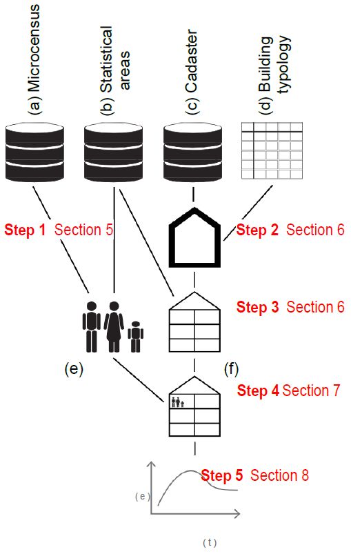
In order to provide the reader with some guidance to the remainder of the document, we offer an overview of the modelling steps and depict the model structure and data sources in Figure 1. We also comment briefly on our modelling philosophy. In constructing our simple model, we perform the following steps:
Step 1. We synthesize the population of “statistical areas” in Hamburg by selecting households from the German Microcensus, fitting them into statistical areas and trying to achieve a good fit of the populations thus synthesized with the aggregate populations recorded for these areas, using a hill climbing algorithm Williamson, Birkin and Rees (1998). “Statistical areas” for Hamburg are areas of up to around 2000 people (in some cases far less) for which fairly detailed sociodemographic data is available (e.g. number of inhabitants per age class). For now we use the Microcensus of 2002; in a later step we plan to use the 2010 data-set. The 2002 Microcensus of Germany contains over 25000 records of individuals in their household contexts and lists around 340 variables, including demographic household composition, employment status, and type of building the household is living in. Step 1 is described in Section 5 of this paper.
Step 2. We equip buildings that are geo-referenced in the official digital Hamburg cadaster with energy-relevant properties. We do this by using the IWU building typology (IWU is the Institute for Housing and Environment in Darmstadt), the leading German building typology developed and continually updated for the purpose of energy assessment of buildings Loga, Diefenbach, Stein and Born (2012). We assign buildings in the digital Hamburg cadaster to types in this typology, using an automated method containing stochastic elements, described in Munoz Hidalgo and Peters (2013). This is the subject of Section 6 in this paper.
Step 3. For the statistical areas, we obtain the number of dwelling units per multi-family building as follows: We add the number of single-family residences (indicated in the cadaster) and an imputed number of dwelling units in multi-family houses, where we impute the latter by dividing the entire floor space of multifamily-buildings (available from the cadaster) through the number of households minus the number of single family residences. This step is described in Section 6 of this paper.
Step 4. For the statistical areas, we assign households (from Step 1) to dwelling units (from Step 3) by using variables from the Microcensus pertaining to the type of building that the house- holds taken from the Microcensus live in. Step 4 is described in Section 7 of this paper.
Step 5. We simulate heat consumption of buildings by using a static heat balance computation tool and varying the parameters pertaining to the occupants (e.g. air exchange, indoor temperature etc.). Usually, in these static tools (as they are used and normal in German legislation for building energy efficiency) the computation is carried out for a normal occupant with normal behaviour, and only the physical building characteristics vary according to the building being assessed. This is to ensure equal assumptions for all building computations. We vary these “occupant variables” based on data from the Microcensus pertaining to work hours which are computed based on employment status, job type, etc. Step 5 is described in Section 8 of this paper.

Model data structure and simulation steps.
The diagram shows the three main databases (a-c) and the additional building typology used for the classification of the building stock (d). In step 4 the synthetic families (e) are merged with the constructed dwelling units (f). The simulation of heat consumption is performed in step number 5.
The model architecture is object-oriented (implemented in Python), representing each individual unit as an object of a “class”. Many authors developing microsimulation models argue in favor of a truly object-oriented model Ballas, Clarke and Turton (1999), Miller, Douglas Hunt, Abraham and Salvini (2004), Rahman, Harding, Tanton and Liu (2010). Having an object-oriented architecture provides the ideal platform for developing an agent-based model, a model type capable of generating emergent phenomena arising out of the interaction of individuals Birkin and Wu (2012). There are not only advantages for the simulation itself, but also for the code, as it becomes more “realistic” and hence less error-prone and easier to share. We see the combination of this (and similar approaches e.g. Cellular Automata) as the most effective method and we therefore prepared our model for our future work as a hybrid agent-based spatial microsimulation model (as did Peters, Brassel and Spörri (2002) for a waste water application).
3. The digital cadaster and the microcensus
In this section we present the main data sources used for our model so far. The different data sources displayed in Figure 1 are: (a) The German Microcensus from 2002; (b) cross tabulation data aggregated to statistical areas for the city of Hamburg; (c) the digital cadaster of the city of Hamburg and d) a building typology developed by the IWU institute for the classification of the German building stock.
The census data comes from the official German Microcensus for scientific research Amtliche Mikrodaten für die wissenschaftliche Forschung NRW, Statistisches Landesamt Geschäftsstelle, F.D.Z. (05.12.2002), developed and maintained by the German Statistical Office of the German Federal Level and the Federal States, Research Data Center Statistische Ämter des Bundes und der Landers, Forschungsdatenzentren. The data set from 2002 contains 25,137 records of individuals in their household contexts and lists around 340 variables for each of these individuals, including the demographic household composition in which they live, their employment status, and type of building the household is living in.
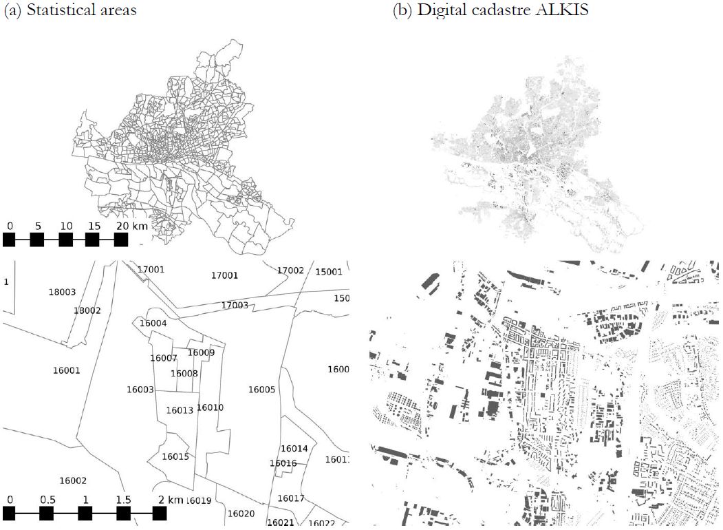
The cross tabulations of statistical areas. Statistical areas (in German: “Statistische Gebiete”) are areas of up to around 2,000 inhabitants for which fairly detailed data on sociodemography are available. This data is developed and maintained by the Statistical Office of the combined Federal States of Hamburg and Schleswig-Holstein. Statistisches Amt für Hamburg und Schleswig- Holstein (StaNord)1 See Figure 2a for the partitioning of Hamburg in statistical areas.
The digital cadaster of Hamburg, the ALKIS2 contains a lot of information on the building stock of the city. Each building is geo-referenced and contains a set of attributes. From these attributes we use both the geo-reference (to estimate living space and building orientation) and the attributes to estimate energy relevant properties of the individual buildings, through the use of a building typology (see d below). See Figure 2b for the buildings recorded in the digital cadaster of Hamburg.
We make use of the building typology developed by Loga et al. (2012) for the German building stock. This typology is well documented and allows the extraction of relevant data. We classify the entire building stock of the digital cadaster into building types of this typology, thereby assigning (1) U-values for the building components (roof, walls and windows) and (2) glazing area, for the estimation of heat loses and solar gains.

Spatial data used in our model.
(a) Statistical areas `Statistische Gebiete’’ containing aggregated sociodemographic information. Statistisches Amt für Hamburg und Schleswig-Holstein (StaNord); and (b) Digital cadaster ALKIS `Amtliches Liegenschaftskatasterinformationssystem’’. Landesbetrieb Geoinformation und Vermessung – Stadt Hamburg (2010).

Occupant influence on different building typologies arrange by construction year.
4. Computing heat demand vs. simulating heat consumption: State of the art in urban heat modelling, and our contribution
Assessing the heat use of buildings can essentially be achieved by two methods, which exist in different variations. Simply speaking, heat demand is computed by constructing a static heat flow balance (or heat accounting balance). German regulations for building energy efficiency employ this approach and define a legally binding procedure, along with parameter values on the occupant, to implement the regulation. See DIN V 18599 Deutsches Institut für Normung e. V (2011). By contrast, there is also dynamic thermal simulation, taking account of spatial-temporal heat flows in the building and detailed circumstances, including occupant characteristics. The latter is the most common method used in the building simulation community Hensen and Lamberts (2011) which is dominated by physicists and engineers.
Thus, demand usually means a hypothetical figure computed in a static energy balance from energy-relevant properties of the building, assuming a normal occupant. Consumption, on the other hand, is what a building actually consumes – a real or a simulated figure that reflects real world deviations from the norm, caused by, for example, occupant attributes and behaviour that deviates from the norm. One could distinguish a third specimen of model used by economists and social scientists, a statistical approach, relating energy consumption to building occupants (or building characteristics) based on observed consumption data, without explicitly accounting for heat flows.
Our ultimate objective is to simulate heat consumption. For this model, therefore, we take a simple approach, using a static heat accounting tool which traditionally is used to assess heat demand, in which we vary the assumptions based on the occupants of the building, such as interior heat gains, air flow, and desired indoor temperature.
Other attempts to perform a simulation of energy consumption at an urban scale using micro units have been performed by Haldi and Robinson (2011), Chingcuanco and Miller (2012) and Druckman and Jackson (2008). Haldi and Robinson (2011) develop their own urban energy demand model (CitySim), which implements a simple thermal simulation, accounting for varying occupants (for more detail see Robinson and Haldi (2011), Page, Robinson, Morel and Scartezzini (2008), Page, Robinson and Scartezzini (2007)), describing the occupants’ presence model which is central to our own approach. The model can be extended to simulate entire urban areas. The authors make use of a Markov-Chain model for generating occupancy rates, thus representing a possible spread of heat demand patterns at an urban scale. It is our aim to expand these approaches, applying the concept of spatial microsimulation to connect demographic characteristics of an urban area, allowing us to observe specific spread patterns of heat demand of the corresponding urban areas. Chingcuanco and Miller (2012) attempt to combine a simulation model (ILUTE)3 working at a micro level with an energy balance model developed specifically for the region under analysis. The first simulation model delivers much of the required data for the heat accounting model.
The study of the influence of occupant characteristics and occupant behaviour on energy demand has a long tradition in economics Scott (1980), Van Raaij and Verhallen (1983a,b), Bohi and Zimmerman (1984). A general problem of these studies is the level of aggregation in the data which records energy consumption across a group of consumers with different characteristics, often not in panel-data format, and often fails to control for the quality of the building (because that data has not been available).
The integration of the occupant influence on various types of dynamic thermal building simulation models has also been studied by others. Almost all the scientific work in this field has been performed at a building level. The area of building simulation addresses this topic in a marginal fashion Mahdavi (2011). It is essential for the further development of heat supply infrastructure in urban environments that a clear understanding of heat consumption patterns at a low level of aggregation is achieved.
A clear difficulty with empirical observations of occupant behaviour influencing energy demand is the need to control for all relevant factors Yu, Haghighat, Fung and Zhou (2011). An important factor for the simulation of energy demand seems to be occupant presence Guerra Santin et al. (2009), the latter authors observing this effect in their work, Page et al. (2008) developed an interesting method for the integration of this parameter into simulation models. The authors simulate a time series of occupants’ presence using a stochastic model. Widén, Molin and Ellegård (2011) make an interesting contribution on the use of time-use data for the modeling of occupant influence in the residential sector. Further methods to integrate occupant behaviour into energy simulation models have been developed Borgeson and Brager (2008), Hoes, Hensen, Loomans, de Vries and Bourgeois (2009), Hensen and Lamberts (2011), Lüdemann (2001), Nouidui, Wetter and Zuo (2012). Table 1 is a rough cut at the literature, classifying modelling approaches reported there and illustrating where our approach is placed.
Different types of models for energy simulation of buildings.
| Model Type\Occupant Type | Static heat balance model (at individual building level) | Dynamic thermal simulation model (at individual building level) | Statistic model relating heat consumption to occupants, at various levels of aggregation, no heat balance imposed |
|---|---|---|---|
| “Average Occupant” (household comprised of identical norm persons; only their number counts) | Blesl, Kempe, Ohl and Fahl (2007), Deutsches Institut für Normung e. V (2011), Dascalaki, Droutsa, Balaras and Kontoyiannidis (2011), Loga, Diefenbach and Born (2011) | EnergyPlus Development Team (2012), Henden and Lamberts (2011) | |
| Household with individualized demographics and behaviour | Chingcuanco and Miller (2012) Munoz & Peters (2014) | Lüdemann (2001), Borgeson and Brager (2008), Page et al. (2008), Mahdavi (2011), Widén et al. (2011). | Scott (1980), Bohi and Zimmerman (1984), Guerra Santin et al. (2009). |
Returning to our approach which uses a static balancing tool to compute heat demand, but varying parameters that may be influenced by the occupants: Figure 3 shows occupant influence on 36 buildings. We calculated the heat demand for each of these buildings varying “occupant parameters”. The variation representing occupant behaviour is performed by the combination of three key input variables: (1) qi[W /m2] = Internal heat emissions; (2) Ti[C◦] = Internal temperature; and (3) n[h−1] = Air exchange rate. In the plot the buildings are arranged by construction period (from oldest to newest). We vary the quality of the building shell along with the construction period. Newer buildings have a better insulated shell. It is clear that the influence of occupant behaviour (measured as relative heat variation ΔQh in percent) is highest on newer buildings.
This literature shows that the integration of occupant behaviour into building simulation models can be achieved. Difficulties arise with the validation of such simulations, as empirical data at the needed temporal and disaggregation resolution is still very hard to get.
5. Constructing synthetic populations for statistical areas
The selected households for the specific “statistical areas” come from the official German Microcensus (see Section 3).
We select entire households from the Microcensus data base set and fit them (with an algorithm described below) into a statistical area such that the aggregated sociodemographic data of this area are matched. We are interested in households rather than individuals, as in the next step we will allocate these households into dwelling units.
Table 2 shows the six variables that we use to fit the households into the statistical areas. Of these six variables, two are taken directly from the Microcensus, and four we computed based upon other variables of the census. We use a combinatorial optimization, Hill Climbing (HC), algorithm to fit households from the micro census into statistical areas, following the method presented by Williamson et al. (1998), Harland, Heppenstall, Smith and Birkin (2012).
Variables used to fit households from the Microcensus into statistical areas.
| Constructed variables | |
|---|---|
| Variable ID | Variable Name |
| Average household size (No. of individuals per dwelling unit) | |
| Number of single households | |
| Number of households with children | |
| Number of single parent households | |
| Variables directly taken from the micro-census | Variable Name |
| ef455 | In what year was your home built? |
| ef451 | How many dwelling units has the building in which you are living? |
-
Source: MIKROZENSUS 2002 Statistisches Bundesamt (2002). Variable names: translation by the authors.
The TAE is calculated, for each statistical area, by forming a weighted sum of the absolute errors of the household variables of Table 2. See Equation 1 for the computation of the TAE and Equation 2 for the computation of the weights. Referring to Table 2, the variable ef455 has nine possible values (corresponding to 9 construction periods), and Variable ef451 has four possible values (corresponding to 4 classes of numbers of dwelling units in the building the individual lives in).
The errors for all variables (except “average household size”) are computed based on the number of families in the specific value class of that variable. This would not make sense for the variable “average household size”. The error for the latter is computed differently, based on the total number of families in the specific area.
Where:
TAEi Total Absolute Error of statistical area i
Estimated variable k for statistical area i, where k = 1,…, 6
Observed variable k for statistical area i
Weight factor of variable k for statistical area i
NIi Observed number of individuals for statistical area i
HHSi Observed average household size for statistical area i
The variable “average household size” receives a smaller weight than the other variables because otherwise it would exert an inappropriate influence on the fitting process. The division by 2 is an ad hoc choice that seems to smoothe the computation process well.
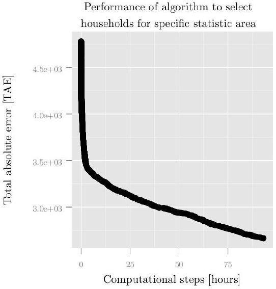
In each simulation step, we randomly exchange one household fitted into the statistical area from a previous random step. If this lowers the TAE, we leave the household in the statistical area; otherwise this exchange is rejected and the simulation continues with another exchange of households. A clear disadvantage of this algorithm is the required computational time. Figure 4 shows the reduction of TAE over time. We can clearly see that the simulation does not achieve an idle state even after 10e+6 iterations steps and more than 3 days of computational time. There are many options to reduce computational time, including the addition of restrictive parameters for the fitting of households in the statistical areas, or the use of a different algorithm to fit the families into the statistical areas.

Performance of the algorithm used for selecting households to fit aggregate values of statistical area 16004.
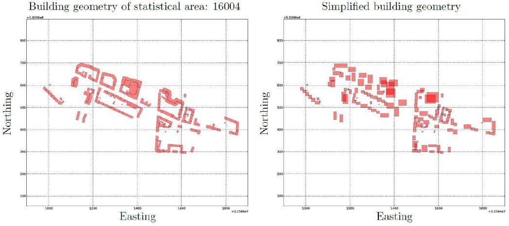
Geometrical simplification of selected buildings (left) original geometry; and (right) simplified geometry used as input for the estimation of heat demand.
(left) original geometry; and (right) simplified geometry used as input for the estimation of heat demand
6. Assigning heat-relevant properties to geo-referenced buildings
For a heat accounting model of individual buildings, certain building data has to be available, foremost building geometry and quality of the building shell. Although the digital cadaster of Hamburg (see Section 3), contains many useful data, it is lacking some heat-relevant data – most importantly, U-values (that is: heat transmission coefficients) of the building shell elements.
The use of building typologies to fill this information gap is an interesting option. National building typologies are constructed with the aim of developing bottom-up models for the evaluation of retrofitting options for the national building stock TABULA Project Team (2012), thus promoting energy-efficiency measures in the building stock at a national level Kragh and Wittchen (2013), Singh, Mahapatra and Teller (2013), Dascalaki et al. (2011). In this paper we make use of the IWU building typology developed by Loga et al. (2012) for the German building stock (see Section 3). We classify the residential buildings recorded in the digital Hamburg cadaster into the types of this specific typology.
The main difference between an analysis of the national building stock, for which the building typologies are developed, and a computation of heat consumption of small areas for the planning of decentralized energy supply systems, which is the scope of our research, pertains to scale. While the former focuses on the aggregate effect of energy-efficiency measures in the building stock, abstracted from its location in space, the planning of decentralized energy supply needs to:
allocate the heat demand on small urban areas, suitable for small decentralized energy supply systems; and
identify areas with a high heat demand density in urban areas in order to allow the prioritizing of retrofits. For the proper dimension of heat supply systems the estimation of heat demand is a key issue, especially at a low aggregation level. The results of using building typologies for the simulation of heat demand improves as the number of buildings are summed together Blesl et al. (2007). This is because many key variables like internal heat gains, internal temperature, ventilation rates, thermal bridges, etc., cannot be identified for every single building. In order to perform the heat demand computation, authors have to use average values defined in national guidelines. For the construction of the typology, authors classify the buildings by a number of variables, such as construction period and construction type (single family house, terrace house, etc.) Kragh and Wittchen (2013), Singh et al. (2013), Hrabovszky-Horváth, Pálvölgyi, Csoknyai and Talamon (2013), Caputo, Costa and Ferrari (2013).
The data from the digital Hamburg cadaster that we are using is a snapshot of the year 2010. With the available information of the digital cadaster we classify the buildings into types of the IWU building typology (see below). From this typology we extract specific data of the building that is not available in the digital cadaster. From the digital cadaster we extract the following variables:
Building use (i.e., residential and various types of commercial);
Land use;
Construction type (i.e., single family house, small multifamily house, row house, etc.);
Construction year;
Building footprint area;
Number of floors; and
Roof type
(1 and 2) – The first two variables, building use and land use, are important in order to filter nonresidential buildings from the database.
(3) – Construction type, is used to filter constructions that have a residential use but are not necessarily heated, at least not with the same intensity as normal living space. So, for example we filter all the garage floor area from our analysis with this variable.
(4) – Construction year, is the most commonly used, especially for the German building stock. This is because in Germany the quality of the building shell has been regulated since the first “Wärmeschutzverordnung” (WSVO) Heat conservation ordinance in 1977. Since its first introduction, the German government has systematically introduced new regulations over the past decades. This has resulted in substantial differences in the quality of the building shell over the years. This variable is also used for the allocation of families into the constructed dwelling units of the building (see Section 7).
(5 and 6) – The floor space plays a key role in the calculation of heat demand, as the floor space can be regarded as heated space. From the digital cadaster we cannot directly recover the floor space. We estimate floor space the same way for all the buildings in the digital cadaster, as follows:
where; sqmi is the living space in m2 of building i; groundareai is the polygon area of building i in the digital cadaster or building footprint; stories is the number of stories of building i; and κ is a constant 0.6, differentiating construction space (exterior end internal walls) from living space or floor space. The number of floors and the roof type are directly retrieved from the digital cadaster. Both parameters are used to define the building geometry.
(7) – Some of the attributes available in the digital cadaster are not available for the entire building stock in the AKIS database, for example, the construction year. This poses a particular challenge, as the construction period is one of the key variables to classify a building. To address this, we have developed an algorithm that filters buildings based on their attributes (including the attributes described above as well as roof type) and calculate the most probable building type that a building belongs to. In extreme cases where just few attributes of the building are available, a type is attributed to the building at random. This process is described in Munoz Hidalgo and Peters (2013).
7. Allocating households to dwelling units in the building stock
For each statistical area we have:
a set of buildings from the digital Hamburg cadaster; and
a set of households fitted to this statistical area.
Now we have to allocate the households into the buildings. We do this via dwelling units, that is, populating dwelling units (located in buildings) with our households. The ALKIS does not give us dwelling units, but we know the total number of dwelling units from the demographic data at statistical area level, and so we estimate dwelling units per building, as follows:
Where:
Si Average Dwelling unit size of multi family buildings in statistical area i
Bsqmi,j,multi Floor space of multi family building j in statistical area i
Hi Number of households in statistical area i
Bi,single Number of single family buildings in statistical area i
qi Calibration factor for statistical area i
We compute the average dwelling unit size of multi-family buildings for the specific statistical area. Then, for each multi-family building, we divide the entire building floor space by the average dwelling unit size mentioned above, round up the result, and we arrive at the estimated number of dwelling units in each building. Because we only allow integers for the number of dwelling units, the total number of dwelling units may differ from the total number of households. This may be seen as realistic, as there may be some vacant dwelling units in the statistical area. The other possibility, that there are not enough dwelling units for the households in the area, may also arise during the simulation. To solve this problem, we implement a factor in the computation of the average dwelling unit size specific for each statistical area. For now this factor only aims to reduce the number of vacant dwelling units. The possibility that there is more than one household in a dwelling unit is ruled out by definition, as the people living together in a dwelling unit count as one household.
After we compute the number of dwelling units in the statistical area, we populate them with the selected households (see Section 5). For this allocation we again use a hill climbing algorithm. First we randomly populate the dwelling units (one household per dwelling unit), then we compute a specific total error for each dwelling unit. The sum of errors is the total absolute error (TAE2) for the statistical area. In an iterative process we start changing households from one dwelling unit to another (always in pairs, household A is allocated in dwelling unit B and household B in dwelling unit A). If the change results in a decrease of the total absolute error, the change is accepted, otherwise the change is rejected and the algorithm draws two new households at random. The variables used to compute the total absolute error are listed in Table 3.
Variables used for the allocation of the synthetic households into the semi-synthetic dwelling units.
| Living standard of the household | |
|---|---|
| Variable ID | Variable Name |
| ef451 | How many dwelling units has the building in which you are living? |
| ef453 | What is the floor area of the dwelling unit? |
| ef455 | In what year was your home built? |
-
Source: MIKROZENSUS 2002 Statistisches Bundesamt (2002). Variable names: translation by the authors.
Because we have fit the synthetic households to characteristics of the building stock (see Table 2 and Section 5), the allocation of households into the building stock should work relatively smoothly. Because in this step we don’t introduce any new families (as in the previous application of the algorithm), the number of possible combinations is limited, although still large enough to allow the implementation of a combinatorial optimization method. The algorithm performs 10e+10 iterations. Its performance is depicted in Figure 6. Because the variables used to merge the households with the dwelling units refer to the building rather than to the dwelling unit within the buildings, changing households are always selected from different buildings and not only just from different dwelling units. The total absolute error (TAE2) is computed as in Equation 5; the corresponding weight for each variable is computed individually for each statistical area as in Equation 6.
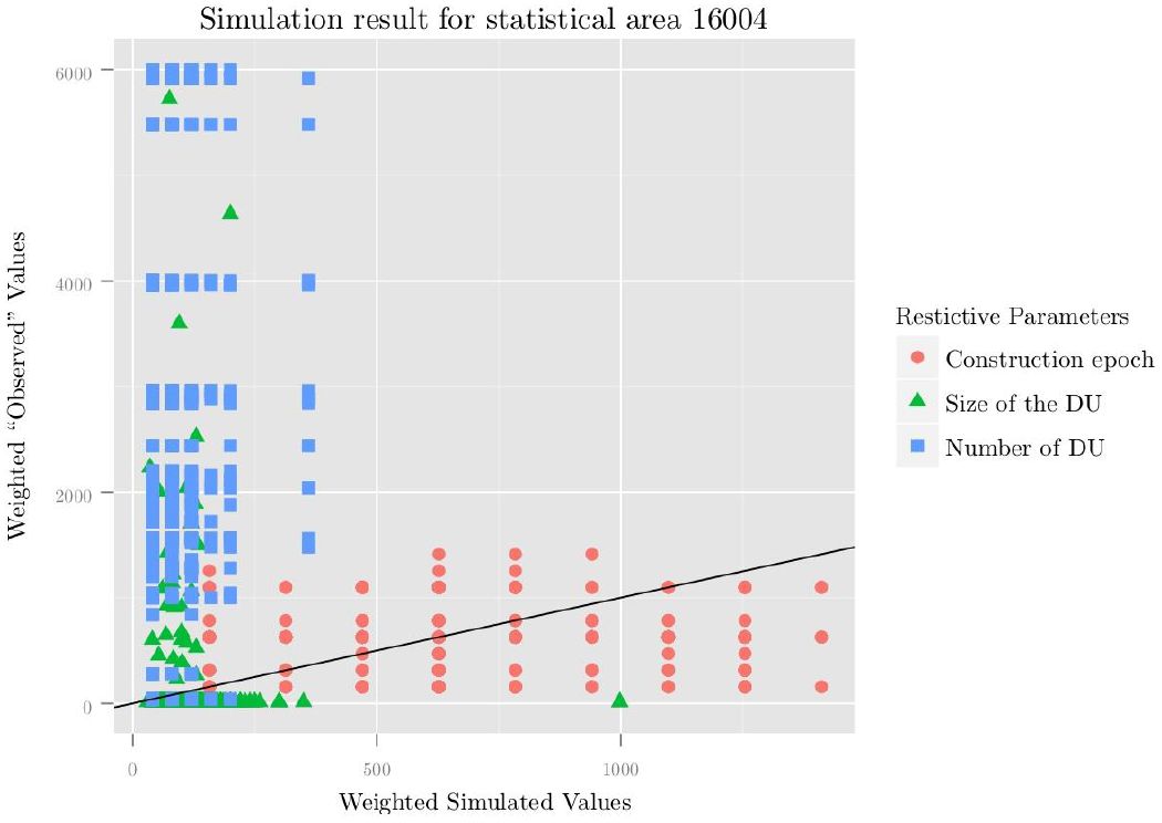
Comparison between simulated and observed parameters.
These Parameters are used as restrictions to merge the households to the dwelling units in statistical area 16,004. Result after 10e+6 (Selection of households from the micro census) + 10e+6 (merge of households with dwelling units) iterations.
Where:
TAE2i Total Absolute Error (Application 2) of statistical area i
Estimated variable l for statistical area i where l = 1 … 3
Observed variable l for statistical area i
Weight factor of variable l for statistical area i
Average variable l for statistical area i
The difference between the simulated households, allocated in the dwelling units, and the “observed” values retrieved from the ALKIS database, is depicted in Figure 6. Because the “observed” values have been partly estimated, we may describe them as semi-synthetic, as the ALKIS database does not have a construction year for all the buildings, the size of the dwelling units has been estimated (except for the single family houses), as has been the number of dwelling units per building.
8. Simulating heat consumption with synthetic microdata
For the simulation of heat consumption we need two sets of input parameters, the first corresponding to the building characteristics and the second corresponding to the individuals living in this building. (For a computation of heat demand, we would need only the first set of input data.) For the buildings and their energy-relevant properties, we use the Hamburg cadaster whose residential buildings we classify into types from the IWU typology (as described in Section 6). From the building typologies of the digital cadaster we compute the following parameters that are used as input to the heat accounting method: (1) Building dimensions, as absolute northing and easting displacement difference, thus implying an orientation of the building; (2) Building height, as number of stories times 3 meters, needed for the computation of the envelope area; (3) Roof slope, estimated based on the roof type, needed for the computation of the envelope area; (4) Percentage of glazed area, for the computation of transmission losses and solar gains, taken from the attributed building type; (5) U-value for the roof, for the computation of transmission losses, taken from the attributed building type; (6) U- value for the walls, for the computation of transmission losses, taken from the attributed building type; and (7) U-value for the windows, for the computation of transmission losses, taken from the attributed building type.
The input parameters derived from the households’ attributes are: (1) Internal heat emissions qi; (2) Internal temperature Ti; and (3) Air exchange rate n. In order to find values for these parameters, we first estimate the average working hours of the individuals living in the building. Here we make use of the micro census again. In order to estimate the average working hours of the single individuals we use the parameters describe in Table 4. With these parameters, we estimate the working hours of every single individual. Because we use the parameter of working hours as an indicator of presence in the dwelling unit, we take the minimum number of working hours out of the set of all household members, thus aiming to describe the presence hours of the one household member that is at home the most. So, for example, for a family with one parent working full-time and the other parent working part-time, the working hours of the household will correspond to the working hours of the parent working part-time. Another important variable is variable ef163, which describes if one of the individuals belonging to the household works at home. If so, the “working hours” of that individual are set to zero. This parameter can take two different values:
always, which we translate to 0; and
sometimes, which we translate to 0.5, reducing the working hours to half.
Variables used to estimate the time at home for the single individuals.
| Labor participation | |
|---|---|
| Variable ID | Variable Name |
| ef95 | Employment status in the reference week |
| ef138 | Full-time / part-time job |
| ef141 | Full-time / part-time job |
| ef147 | Work on Saturday (February until April) |
| ef148 | Work on Sundays and public holidays (February until April) |
| ef149 | Evening work (between 6 p.m and 11 p.m) (February until April) |
| ef150 | Night work (between 11 p.m and 6 a.m) (February until April) |
| ef151 | Night work hours (between 11 p.m and 6 a.m) (February until April) |
| ef163 | Home office (February until April) |
-
Source: MIKROZENSUS 2002 Statistisches Bundesamt (2002). Variable names: translation by the authors.
Table 4 shows a list of parameters used to estimate the working hours and the hours at home of the household. In the next step an average is calculated for the building (that is, if the building is a multi-family house).
With the estimated working hours of the individual households and the average working hours of the building residents, we create a simple rule to define a set of input parameters for the heat accounting model. This rule distinguishes five different types of households (see Table 5), ranging from: a low temperature, low ventilation rate and low internal gains to the other extreme: with a high temperature demand, a high ventilation rate and high internal gains. The household type in the middle represents the “average” household, its parameter values follow those of the national norms. To these parameters we attach the average working hours (8), and subsequently, short working hours correspond to high ventilation, high temperature rates and high internal gains. In the other extreme, long working hours correspond to low temperature, low ventilation rates and low internal gains.
Rules to select input variables to the heat balance model based on the average working hours in the building.
| Computed work time (wk) | qi[W/m2] | Ti[C°] | n[h−1] | Possible occupant type | ||
|---|---|---|---|---|---|---|
| wt = | > 10 | 3 | 18 | 0.3 | single household, employed | |
| wt = ≤ 9 | ∧ | > 8 | 6 | 19 | 0.4 | both parents employed |
| wt = ≤ 8 | ∧ | > 4 | 5 | 20 | 0.5 | “average” occupant |
| wt = ≤ 4 | ∧ | > 1 | 6 | 21 | 0.6 | part time |
| wt = ≤ 1 | 7 | 22 | 0.7 | unemployed | ||
-
qi[W /m2] = Internal heat emissions; Ti[C°] = Internal temperature; and n[h−1] = Air exchange rate.
We present the result for the selected statistical area (16004) by comparing: (1) the estimated heat demand with help of the “standard” heat balance model, this model assumes an “average” household and so makes uses of the standard internal gains, internal temperature and ventilation rates, corresponding to row 3 of Table 5 and (2) the implementation of the heat balance method, varying input parameters (qi, Ti and n) as a function of the computed average working hours of the building, thus simulating heat consumption. The result of this comparison in presented in Figure 7. One can clearly see in the plot that the simulated heat consumption shows a bigger spread. This is plausible, as it considers a richer spectrum of occupant types. The analyzed statistical area still has a high proportion of “old” buildings, that is buildings predating the first (WSVO) Heat conservation ordinance in 1977 (see Figure 8). We can expect a much higher relative spread in urban areas that have been recently developed or re-developed (“relative” meaning: relative in terms of the overall amount of heat consumption).
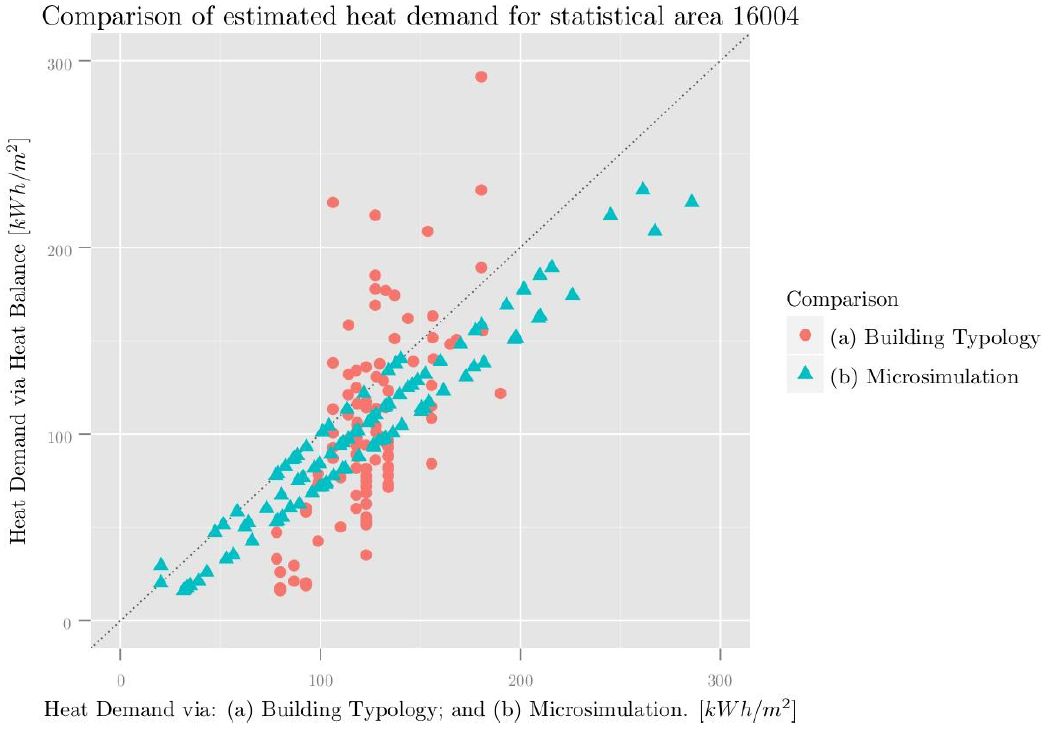

Comparison between estimated heat demand and simulated heat consumption.
Comparison between heat demand estimated with a heat balance method, using the ``average’’ occupant (vertical axis) and with help of: (a) building typologies; and (b) a heat balance, taking into account occupant influence, induce thought the synthetic simulated demographic characteristics via a spatial microsimulation (horizontal axis). This comparison shows the results of buildings in statistical area 16004.
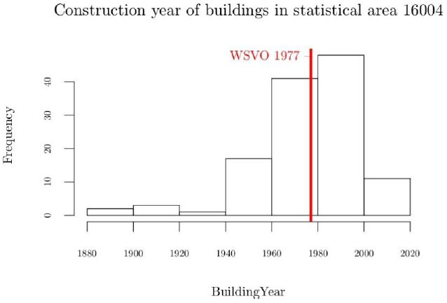

Histogram showing the frequency of construction year in statistical area 16004.
To generate this distribution only known construction years are used.
Description of some parameters of statistical area 16004 in comparison of the average value for the city of Hamburg.
| Statistical area 16004 | Hamburg | Δ | |
|---|---|---|---|
| Size of household [# individuals per household] | 2.0 | 1.8 | 0.2 |
| Share of foreign nationals [%] | 45.1 | 13.6 | 31.5 |
| Share of household with kids [%] | 26.7 | 16.9 | 9.8 |
| Share of unemployed residents*[%] | 12.2 | 4.8 | 7.4 |
| Share of single person households [%] | 49.8 | 51.2 | 1.4 |
| Number of private cars per 1000 residents [cars] | 180 | 353 | 172 |
-
*Residents between the ages of 15 and 65.
On average the simulated heat consumption is much higher than the estimated heat demand. The selected urban area does not represent the average household in Hamburg. Table 6 compares some attributes with the average value for the entire city. The selected area has: (1) a high level of unemployment, which in our model means less or 0 working hours; (2) a lower share of single person households, which raises the probability of having a resident with zero working hours; and (3) a high share of households with children, leading also to low working hours of the household.
9. Next step: Including a thermal simulation model
In a further step we aim to integrate a thermal simulation model. This will allow us to: (1) simulate at a much higher temporal resolution, needed for the efficient dimensioning of decentralized energy supply systems; and (2) feed the model with more detailed input data. The second reason is essential for achieving our goal. Most of the defined energy balance norms or models take a limited number of parameters as input; in particular there are few parameters that are related to occupant behaviour. This is because the aim of the standard method is the estimation of heat demand for the “average” occupant. Because we want to represent the full spectrum of occupants and their corresponding influence on the system we have to make use of a more flexible method for the estimation of residential heat demand.
Because of the nature of the heat accounting model, and the underlying national standard, we have to define a range of occupant-related parameters for each dwelling unit, rather than a time schedule reflecting occupants’ presence. In our model we chose to estimate the average working hours as we plan to extend the model to incorporate a thermal simulation which is able to use a detailed occupants’ presence schedule as input. This means that from variable ef147 onward (see Table 4) we need to generate a detailed schedule for the simulation of heat consumption via a thermal simulation Widén et al. (2011), Wilke et al. (2011).
Another problem with the use of a static heat balancing method is the inability of such a model to integrate individual characteristics of dwelling units. The major problem by attempting a dwelling-unit specific computation of heat consumption is the required input variables regarding the building envelope. In order to perform a dwelling unit based heat computation, we will have to define the geometry not only of the building but of the dwelling unit itself, orientation, size of facade, etc. This problem is no longer present for a proper thermal simulation model as the generated schedule can define various levels of occupancy.
10. Conclusions
The presented results mark our first attempt to simulate heat consumption at an urban scale, using microdata. Our model combines well established implementations from: (a) the microsimulation community and (b) the building simulation community. In this paper we have shown that a combination of both methods is possible and can generate interesting insights into the planning of cities and their technical infrastructures. We use a method from the microsimulation community (the Hill Climbing algorithm) to select families from the census database and allocate them into small statistical areas within the city. From the digital cadaster we attribute the corresponding buildings with energy relevant characteristics. In a third step we allocate the selected families into individual buildings. The buildings with it inhabitants serve as input data to a simplified heat balance model following the German DIN V 18599 standard.
We can show that the integration of socio-demographic characteristics of the families living in a specific area can be used as input for the simulation of heat consumption. This is an important contribution to both scientific communities as: (a) it shows an interesting application of microsimulation in the energy sector and (b) it presents an interesting approach for the building simulation community to integrate the occupants of the buildings into the simulation models not only within a sensitivity analysis but placing the occupant central to the simulation.
Current models for projecting heat demand employ an “average” occupant, both at a building scale and at an urban scale. The trend towards decentralized, as well as more efficient technical systems leads to greater sensitivity of technical systems. An integration of the occupant into infrastructure models will play an important role in the future of urban planning.
With our simplified model we have shown that we are able to indicate a direction in the spread of estimated consumption that is plausible and commensurate with what we know about the analyzed area to which it was applied. As described in Section 9, we expect from future work – integrating a thermal simulation model and constructing a more accurate micro data set – promising results for the energy planning sector. Although this paper focuses exclusively on heat energy, the range of questions that can be analyzed once a population is allocated to buildings is manifold.
Footnotes
1.
2.
3.
Integrated Land Use, Transportation, Environment modelling system.
References
-
1
Exploring Microsimulation Methodologies for the Estimation of Household Attributes4th International conference on GeoComputation.
-
2
Agent-Based Models of Geographical SystemsA Review of Microsimulation and Hybrid Agent-Based Approaches, Agent-Based Models of Geographical Systems, Springer Netherlands, Dordrecht.
- 3
-
4
An update on econometric studies of energy demand behaviorAnnual Review of Energy 9:105–154.
- 5
-
6
A supporting method for defining energy strategies in the building sector at urban scaleEnergy Policy 55:261–270.https://doi.org/10.1016/j.enpol.2012.12.006
-
7
A microsimulation model of urban energy use: Modelling residential space heating demand in ILUTEComputers, Environment and Urban Systems 36:186–194.https://doi.org/10.1016/j.compenvurbsys.2011.11.005
-
8
Building typologies as a tool for assessing the energy performance of residential buildings – A case study for the Hellenic building stockEnergy and Buildings 43:3400–3409.https://doi.org/10.1016/j.enbuild.2011.09.002
-
9
DIN V 18599: Energetische Bewertung von Gebäuden – Berechnung des Nutz-, End- und Primärenergiebedarfs für Heizung, Kühlung, Lüftung, Trinkwarmwasser und Beleuchtung: Berechnung des Nutz-, End- und Primärenergiebedarfs für Heizung, Kühlung, Lüftung, Trinkwarmwasser und Beleuchtung Sonderdruck 2012
-
10
Household energy consumption in the UK: A highly geographically and socio-economically disaggregated modelEnergy Policy 36:3177–3192.https://doi.org/10.1016/j.enpol.2008.03.021
-
11
EnergyPlus Input Output Reference: The Encyclopedic Reference to EnergyPlus Input and Output
-
12
The effect of occupancy and building characteristics on energy use for space and water heating in Dutch residential stockEnergy and Buildings 41:1223–1232.https://doi.org/10.1016/j.enbuild.2009.07.002
-
13
The impact of occupants’ behaviour on building energy demandJournal of Building Performance Simulation 4:323–338.https://doi.org/10.1080/19401493.2011.558213
-
14
Creating Realistic Synthetic Populations at Varying Spatial Scales: A Comparative Critique of Population Synthesis TechniquesJournal of Artificial Societies and Social Simulation, 15, 1, http://jasss.soc.surrey.ac.uk/15/1/1.html.
-
15
Building performance simulation for design and operationAbingdon and Oxon and and New York and NY: SponPress.
-
16
User behavior in whole building simulationEnergy and Buildings 41:295–302.https://doi.org/10.1016/j.enbuild.2008.09.008
-
17
Generalized residential building typology for urban climate change mitigation and adaptation strategies: The case of HungaryEnergy and Buildings 62:475–485.https://doi.org/10.1016/j.enbuild.2013.03.011
-
18
Leitungsgebundene Wärmeversorgung im ländlichen Raum: Handbuch zur Entscheidungsunterstützung Fernwärme in der FlächeLeitungsgebundene Wärmeversorgung im ländlichen Raum: Handbuch zur Entscheidungsunterstützung Fernwärme in der Fläche, http://publica.fraunhofer.de/eprints/urn:nbn:de:0011-n-1136251.pdf.
- 19
- 20
-
21
Development of two Danish building typologies for residential buildingsEnergy and Buildings, 10.1016/j.enbuild.2013.04.028.
-
22
Amtliches Liegenschaftskatasterinformationssystem
-
23
Space-heating and water-heating energy demands of the aged in the 5US6Energy Economics 24:267–284.https://doi.org/10.1016/S0140-9883(02)00014-2
- 24
- 25
-
26
Auslegung, Energiebedarf und Komfort von Anlagen zur Heizung und Warmwasserbereitung im Niedrigenergiehaus bei Berücksichtigung des Nutzerverhaltens. B. Lüdemann, [Bahrenhof and Dorfstr. 13]Auslegung, Energiebedarf und Komfort von Anlagen zur Heizung und Warmwasserbereitung im Niedrigenergiehaus bei Berücksichtigung des Nutzerverhaltens. B. Lüdemann, [Bahrenhof and Dorfstr. 13].
- 27
-
28
Microsimulating urban systemsComputers, Environment and Urban Systems 28:9–44.https://doi.org/10.1016/s0198-9715(02)00044-3
-
29
Allocating heat consumption of residential buildings in space with help of a filter array to determinate the building type in a digital cadaster: Working Paper. Technical Urban Infrastructure Systems GroupHafenCity University (HCU).
-
30
Validation of the window model of the Modelica Buildings libraryProc. of the 5th SimBuild Conference.
- 31
-
32
A generalised stochastic model for the simulation of occupant presenceEnergy and Buildings 40:83–98.https://doi.org/10.1016/j.enbuild.2007.01.018
-
33
Stochastic simulation of occupant presence and behaviour in buildings10th Conference of International Building Performance Simulation Association. pp. 757–764.
-
34
How people use thermostats in homes: A reviewBuilding and Environment 46:2529–2541.https://doi.org/10.1016/j.buildenv.2011.06.002
-
35
A Microsimulation Model for Assessing Urine Flows in Urban Wastewater Management: Integrated Assessment and Decision SupportProceedings of the First Biennial Meeting of the International Environmental Modelling and Software Society.
-
36
Methodological Issues in Spatial Microsimulation Modelling for Small Area EstimationInternational Journal of Microsimulation 3:3–22.
-
37
Modelling Occupants’ Presence and Behaviour – Part II: Journal of Building Performance SimulationJournal of Building Performance Simulation 5:1–3.https://doi.org/10.1080/19401493.2011.599158
-
38
The economics of house heatingEnergy Economics 2:130–141.https://doi.org/10.1016/0140-9883(80)90024-9
-
39
An analysis on energy efficiency initiatives in the building stock of Liege, BelgiumEnergy Policy 62:729–741.https://doi.org/10.1016/j.enpol.2013.07.138
-
40
Datensatzbeschreibung: MIKROZENSUS 2002
- 41
-
42
Directive 2002/91/EC on the energy performance of buildings: Directive 2002/91/ECDirective 2002/91/EC on the energy performance of buildings: Directive 2002/91/EC.
-
43
Directive 2010/31/EU on the energy performance of buildings: Directive 2010/31/EUDirective 2010/31/EU on the energy performance of buildings: Directive 2010/31/EU.
-
44
A behavioral model of residential energy useJournal of Economic Psychology 3:39–63.https://doi.org/10.1016/0167-4870(83)90057-0
-
45
Patterns of residential energy behaviorJournal of Economic Psychology 4:85–106.https://doi.org/10.1016/0167-4870(83)90047-8
-
46
Models of domestic occupancy, activities and energy use based on time-use data: deterministic and stochastic approaches with application to various building-related simulationsJournal of Building Performance Simulation 5:27–44.https://doi.org/10.1080/19401493.2010.532569
-
47
A model of occupants’ activities based on time use survey data2125–2132, 12th Conference of International Building Performance Simulation Association, Sydney, http://www.ibpsa.org/proceedings/BS2011/P_1676.pdf.
-
48
The estimation of population microdata by using data from small area statistics and samples of anonymised recordsEnvironment and Planning A 30:785–816.https://doi.org/10.1068/a300785
-
49
A novel methodology for knowledge discovery through mining associations between building operational dataEnergy and Buildings, 10.1016/j.enbuild.2011.12.018.
Article and author information
Author details
Publication history
- Version of Record published: April 30, 2014 (version 1)
Copyright
© 2014, Muñoz H. and Peters
This article is distributed under the terms of the Creative Commons Attribution License, which permits unrestricted use and redistribution provided that the original author and source are credited.