The MicSim package of R: An entry-level toolkit for continuous-time microsimulation

Cite this article as: S. Zinn; 2014; The MicSim package of R: An entry-level toolkit for continuous-time microsimulation; International Journal of Microsimulation; 7(3); 3-32. doi: 10.34196/ijm.00105

Article
Figures and data
Jump to

Abstract

High entry barriers might discourage many social scientists from using existing microsimulation software. This article presents the functionality and capabilities of the free and open source R package MicSim which allows performing continuous-time microsimulation at a very fine-grained level from a low level entry point. Hence, the package might also be of interest to people who are new to R. The package implements a generic microsimulation model for a wide range of demographic applications. Its central device is the individual life-course, which is defined by the sequence of states the individual visits over time and the intervals between the transitions from one state to another. The MicSim model is by design a discrete-event simulation model in which a demographic event implies a change in the state of an individual. The considered population is open and life-courses are specified to evolve along three continuous time scales: individual age, calendar time, and the time that an individual has already spent in the current state. The stochastic model of the microsimulation is parameterized with a base population, transition rates, and (if applicable) a population of migrants. Besides stochastic events, the package allows specifying deterministic events such as enrolment of children in elementary school. Example applications illustrate the capabilities of the package.

1. Introduction

With steadily growing computer power, microsimulation techniques become increasingly relevant in the social sciences, implying a rising demand of related software. Having, however, to write new software for each new microsimulation application from scratch places enormous and unnecessary burdens on researchers. Recently, researchers have responded to this obstacle by following mainly two strategies. Either they have implemented microsimulation models by using general simulation frameworks such as μsik (Perumalla, 2005; Onggo, 2010) and JAMES II (Himmelspach, 2012) or they have used microsimulation toolkits especially designed for their needs such as the microsimulation language Modgen (Statistics Canada, 2011) and the microsimulation modelling policy tool JAMSIM (Mannion, 2014). (An extensive list of simulation tools relevant in this context is given by, for example, Mannion et al. (2012).) Unfortunately, often the value of simulation frameworks and microsimulation tools is hampered by being both very complex and hard to use or by requiring prior expert knowledge of the software being used. A further impediment of many existing software package is their restriction to specific settings and sets of variables. Obviously, due to the complexity of the issue, an all-purpose simulation standard tool for all kinds of conceivable simulation models and applications is not practicable. Rather, the development of user-friendly and up-to-date microsimulation toolkits tailored to specific areas seems to be the ideal solution. In demography, such toolkits exist, but commonly they assume a certain level of expert knowledge in form of the specification language being used. Thus, to many demographers the first hurdle to take might be too high. For example, the Mic-Core is a continuous-time microsimulation tool for population projections (Zinn et al., 2009). It is written in Java and makes use of the simulation framework JAMES II (Himmelspach, 2012). It features an own graphical user interface and is very performant in terms of run times, allowing for the simulation of thousands of life-courses within a few seconds. However, the Mic-Core demands that the input data (i.e., the base population and the transition rates) are in a very special format that some users might find hard to prepare. In addition, its output data come in a format with which most social scientists are not familiar. For example, the Mic-Core reports birth times and transition times in milliseconds since January 1, 1970.

In this article, we present an easy-to-use, free, and open source toolkit for continuous-time microsimulation tailored to the needs of demographers. We describe the functionality and capabilities of the R package MicSim¹ (Zinn, 2014; R Development Core Team, 2013) which re-implements and extends the model and simulation techniques of the Mic-Core. Compared to the Mic-Core, the MicSim package enables a simplified specification of the microsimulation model and of the input data. As R is becoming the software tool of choice for statistical analysis, it is brimming with up-to-date statistical methods which are free and open source. Thus, the MicSim package allows conducting data preparation and evaluation in a very sophisticated way by using these methods. In addition, the MicSim package extends the functionality of the Mic-Core by facilitating the modelling of a wider class of transition models. On the one hand, the package relaxes the assumption of piecewise constant transition rates, which in the Mic-Core is essential. That is, it allows transition rates to be defined by any parametric and nonparametric function. On the other hand, the MicSim package allows transition rates to vary along age, calendar time, and the time that an individual has already spent in the current state. (The Mic-Core determines transition rates to vary only along age and calendar time.) In other words, all applications that can be run with the Mic-Core can also be run with the MicSim package, but additionally the MicSim package allows performing simulation runs relying on more complex transition models. The new microsimulation toolkit can be downloaded from the R package database and used without further ado. Thus, it is easily accessible and its implementation is traceable. However, not employing Java and JAMES II for microsimulation has its price: opposed to the Mic-Core, the microsimulation routines implemented in the MicSim package are not as performant in terms of run times. The MicSim package addresses this problem by offering a function for distributed computation.²

The topic of this paper is the generic microsimulation model of the MicSim package, and its realization and application. The remainder of the paper is structured as follows. First, in Section 2, we shortly describe the generic microsimulation model that has been implemented, and explain in detail how the functions of the MicSim package have to be specified to obtain viable microsimulation models. All of the general descriptions presented are substantiated by excerpts of two illustrative examples whose source code can be found in the example section of the help page of the micSim function of the MicSim package³. The first (very simple) example deals with gender-specific mortality. The second (more complex) example focuses on individual behaviour concerning changes in marital status, educational attainment, and fertility status. The second example also considers immigration and emigration. In order to better understand the functionality of the package, we strongly recommend running the examples while reading the paper⁴. In Section 3, we present the special features of the MicSim package: Specifically, we demonstrate the simulation of the birth of offspring during the simulation, the modelling of enrolment in elementary school, and procedures for following migrants. Then, in Section 4, we show how to actually perform a continuous-time microsimulation, and we outline the structure of its output. Finally, in Section 5, we provide some concluding remarks and ideas for possible extensions of our package.

2. Microsimulation model

The MicSim package implements a demographic microsimulation model which comprises a stochastic model of individual behaviour and a virtual population. The virtual population consists of a set of individuals who are assigned to attributes which are considered demographically relevant, such as sex, marital status, fertility status, and educational attainment. To each member of the virtual population a birth date is assigned. Commonly, the virtual population resembles a real population structure. It evolves over time as individuals experience demographic events across their lifetimes. For reasons of feasibility, the MicSim microsimulation model is framed by a simulation horizon; i.e., a simulation start date and a simulation end date, and a maximum age up to which each life-course is followed. Modelling and simulating the life-courses of a representative share of population members allows mapping population dynamics on a very detailed scale. Despite the considerable regularity of demographic behaviour, the order- and age-specific incidence of demographic events varies between individuals, and cannot be fully explained by observable characteristics. Thus, in efforts to describe individual behaviour, commonly a stochastic model is applied (Mayer & Tuma, 1990). The most common type of stochastic model used is a continuous-time multi-state model (Andersen & Keiding, 2002; Gampe & Zinn, 2007; Aalen et al., 2008). A multi-state model is a stochastic process that at any point in time occupies one of a set of discrete states (Hougaard, 1999). In the microsimulation model under consideration, these states form the state space. In the following, we describe provide a succinct description of the components of the microsimulation model. In addition, we show the required specifications of these components in the MicSim package.

2.1 The state space

Generally, the state space is determined by the problem to be studied, but often it will at least have “sex” as a basic demographic characteristic. It should be emphasized that, in a continuous-time microsimulation model such as the one considered, age runs parallel to the process time; that is, age evolves in continuous time and is not modelled by means of a discrete variable. In other words, age is not part of the state space. One element always present in the state space is “dead,” a risk to which each individual is always exposed⁵. In the terminology used in the MicSim package, an individual’s state is a combined characteristic, given by the combination of several attributes (if several attributes are considered). To simplify the description, we define so-called state variables. All of the unique combinations of values of these state variables define the state space. Table 1 shows an example comprising six state variables: sex, marital status, fertility status, educational attainment, mortality, and emigration. Throughout this paper, we rely on extracts of this example (whose full specification is part of the help page of the micSim function of the MicSim package).

Table 1

Example state space: State variables and their corresponding values. (Value labels, subsequently used, are given in parentheses)

State Variable	Possible Values
Sex	Female (f), male (m)
Marital status	never married (NM), married (M), divorced (D), widowed (W)
Fertility status	childless (0), one child (1), two children (2), three and more children (3+)
educational attainment	no education (no), primary education only (low), lower secondary school (med), upper secondary or tertiary education (high)
Mortality	Alive, dead (dead)
Emigration	Not emigrated, emigrated (rest)

For example, (female, married, childless, lower secondary school) is one potential state in this state space. Exceptions to this rule are the attributes “alive” and “not emigrated,” which are not explicitly listed for obvious reasons; and the attributes “dead” and “emigrated,” which themselves denote states. “Dead” and “emigrated” are both absorbing states that, once they have been entered, will never be left again. All of the other states are nonabsorbing; they can, at least potentially, be left again⁶.

The MicSim package requires the specification of the nonabsorbing states of the state space in the form of a data frame. Each column of this data frame defines one state variable, and each row gives one potential nonabsorbing state. Hence, in sum, the data frame comprises as many rows as unique combinations of nonabsorbing values of state variables exist. All of the state variables considered, as well as the accordant value labels, have to be provided by the user. The only exception is sex, which is predefined by the labels “m” and “f,” indicating male and female individuals. Furthermore, the label values “no” and “low” are reserved for enrolment in elementary school (see Section 3.2). The simplest state space that the MicSim package can handle has only sex as a state variable. (The full specification of the accordant working example is also given in the help page of the micSim function of the MicSim package).


R> sex <- c("m", "f")
R> stateSpace <- sex
R> attr(stateSpace, "name") <- "sex"

Here and in the subsequent, the prefix R> denotes a command to R. Line breaks within commands are marked by the sign +. The user should be aware that for further processing, MicSim requires a name for each state variable. Names are created by assigning an accordant attribute to stateSpace. The following command determines the (nonabsorbing) states of the example state space given in Table 1.


R> sex <- c("m", "f")
R> fert <- c("0", "1", "2", "3+")
R> marital <- c("NM", "M", "D", "W")
R> edu <- c("no", "low", "med", "high")
R> stateSpace <- expand.grid(sex = sex, fert = fert,
+ marital = marital, edu = edu)

At this point, the R function expand.grid (part of the basic configuration of R) helps in building up the state space by creating a data frame from all of the combinations of the values of the supplied vectors. Absorbing states have to be given as strings, such as “dead” for being dead or “rest” for having emigrated. They are specified by means of a vector named absStates.


R> absStates <- c("dead", "rest")

If out-migration of the population is not considered, absStates reduces to


R> absStates <- "dead"

2.2 Simulation horizon and maximum age

Each simulation model demands the specification of a simulation start date, as well as a simulation end date. Furthermore, the maximum age to which the life-courses are followed has to be determined. In the MicSim package, the simulation horizon is set using the function setSimHorizon. This function has two arguments: the simulation start date and the simulation end date. Both have to be given as strings of the format “dd/mm/yyyy;” for instance,


R> simHorizon <- setSimHorizon(startDate = "01/01/2000",
+ endDate = "31/12/2050")

The maximum age up to which individuals are followed is determined by the scalar maxAge and has to be an integer number of years; for example,


R> maxAge <- 100

2.3 The virtual population

The virtual population consists of all of the individuals who are considered during the simulation. It can be regarded as a longitudinal sample from a synthetically constructed population that resembles a real one. Each individual enters the virtual population in a state that is an element of the state space. Usually, there are three possibilities for becoming part of the virtual population:

by being a member of the base population at the simulation start date,
by birth during simulation, or
by immigration during simulation (if the model includes immigration into the population).

The base population comprises information about the distribution of individuals according to birth dates and to the states they occupy at simulation start date. This information has to be given by the user. MicSim expects the base population to be provided in form of a data frame. Each row of the data frame corresponds to one individual with the following information: a unique numerical person identifier (ID), a birth date (birthDate), and an initial state (initState); that is, the state occupied by the individual when entering the virtual population. Birth dates have to be chron objects. Initial states are given in the form of composites of the labels of the values of the state variables previously specified when defining the state space. Within each initial state the ordering of the state variables has to be equivalent to the ordering determined when defining the state space. Within states, labels are separated by a forward slash “/”. We illustrate the composition of an initial population using a very simple setting with only five individuals who are distinguished only by their gender and their birth date⁷


R> dts <- c("31/12/1930", "03/04/1999", "15/10/1956",
+ "11/11/1991", "01/01/1965")
R> birthDates <- chron(dates = dts, format = c(dates = "d/m/Y"))
R> initStates <- c("f", "m", "f", "m", "m")
R> initPop <- data.frame(ID = 1:5, birthDate = birthDates,
+ initState = initStates, stringsAsFactors = FALSE)

(Here, we have to be careful to ensure that R does not convert strings into factors when constructing the data frame, by using the command stringsAsFactors = FALSE.)

We yield the following base population:


ID birthDate initState
1 31/12/30 f
2 03/04/99 m
3 15/10/56 f
4 11/11/91 m
5 01/01/65 m

To yield meaningful population projections, it is generally advisable to use census data or data of representative cross sections to construct base populations.

If the microsimulation model considered assumes female fertility resulting in offspring (see Section 3.1), newborns might enter the virtual population over the course of the simulation period. These newborns also have to be assigned to the state space. Obviously, most states do not apply, as newborns are always childless, have no education, and so on. In order to determine those states that can actually be initial states of newborns (denoted as initStates), according occurrence probabilities need to be defined. Newborns are then randomly assigned corresponding to these states according to their occurrence probabilities⁸. Usually, simulation models that allow for the creation of newborns employ an empirical sex ratio (the number of male newborns relative to the number of female newborns) to determine a newborn’s sex. This has to be taken into account when setting the occurrence probabilities of the possible initStates. An example is the subsequent setting for the example state space of Table 1.


R> initStates <- rbind(c("m", "0", "NM", "no"),
+ c("f", "0", "NM", "no"))
R> initStatesProb <- c(0.517, 0.483)

Here, we assume a sex ratio of 51.7 male newborns to 48.3 female newborns, as well as (male, never married, childless, no education) as the initial state for male newborns and (female, never married, childless, no education) as the initial state for female newborns. By default, MicSim states that initStates = c() and initStatesProb = c(); that is, if not specified otherwise, it assumes that along simulation time no newborns enter the virtual population.

The microsimulation model of MicSim is per se an open population model; that is, it allows for immigration. Immigrants have to be assigned to the state space when entering the virtual population. Furthermore, for each migrant a birth date has to be given. As in the case of the base population, information about immigrants has to be given in the form of a data frame (immigrPop). Each row of the data frame corresponds to one immigrant. The data frame immigrPop has to contain the following data: a unique numerical person identifier (ID), an immigration date (immigrDate), a birth date (birthDate), and an initial state (immigrInitState); that is, the state occupied by the immigrant when entering the virtual population. Immigration dates and birth dates have to be chron objects. Coming back to our example of Table 1, a potential set of migrants could be defined by


ID immigrDate birthDate immigrInitState
10001 11/Mar/2027 10/Mar/1981 m/1/NM/low
10002 25/Apr/2021 09/Mar/1973 f/1/W/low
10003 19/Jan/2032 29/Dec/2013 m/0/NM/no
10004 15/Jul/2024 12/Aug/1989 f/0/M/high
10005 15/May/2017 23/Nov/1991 m/1/D/med
10006 20/Jan/2014 16/Sep/1964 m/3+/M/high
...

It is important to note that numerical person identifiers have to be unique. Hence, IDs for migrants are given depending on the size of the base population. If, for example, we have a base population of size N=10000, then the first ID that can be given to a migrant is 10001. As in the base population definition, the initial states of migrants have to be strings (not factors). By default, the MicSim package does not assume immigration into the virtual population; that is, immigrPop = NULL. The generic model of MicSim allows for following migrants once they have entered the virtual population. The respective processing is described in Section 3.3.

Individuals can leave the population either by death or by emigration (if emigration is allowed). MicSim handles both types of events by asking for accordant transition rates; see Section 2.3.4.

In its current version, the MicSim package does not require the base population and the data on immigrants to include any information about the amount of time individuals have already spent in their initial states. Such a setting is appropriate if we assume that the waiting times already spent in the initial states do not affect any upcoming events. Nonetheless, the situation is different if we assume state duration dependence; that is, if we employ semi-Markov processes to describe individual behaviour (cp. Section 2.4.1). Here, it is usually incorrect to simply ignore the length of time individuals have already spent in their current states when entering the virtual population. A failure to take this time period into account might lead to a distortion of the duration effects when determining the first events of members of the base population and of immigrants. We will return to this issue in our conclusion when we elaborate on the work in progress and list further possible extensions of the MicSim package.

2.4 Stochastic model of individual behavior

2.4.1 Modeling life-course events over age, calendar time, and time elapsed

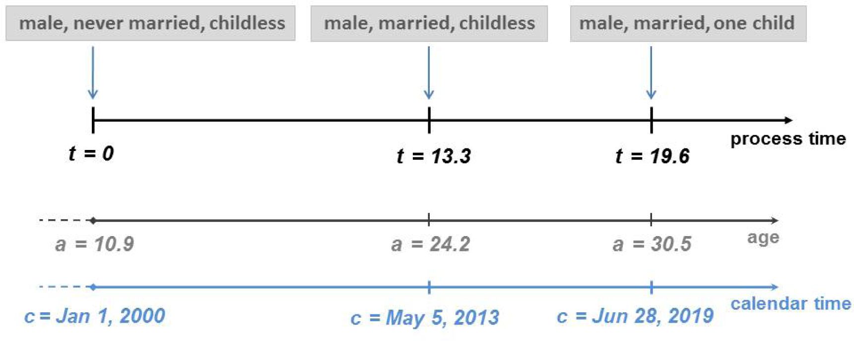
In a continuous-time microsimulation such as the one considered in the MicSim package, individual life-courses are usually specified by sequences of state transitions (events) and the time spans between these transitions. A common way to characterize an individual life-course is by means of a continuous-time multi-state model; that is, an individual life-course is described by a stochastic process $Z (t), t \in R_{0}^{+}$ , usually from the family of Markovian processes (Kijima, 1997). Here, the process time t maps the time span over which we “observe” an individual life-course. The time t is set to zero when an individual enters the virtual population. As long as the individual is part of the virtual population, t evolves along the individual lifetime. Individual age and calendar time are simple translations of the process time. Figure 1 shows a part of a potential synthetic life-course.

Figure 1

Download asset Open asset

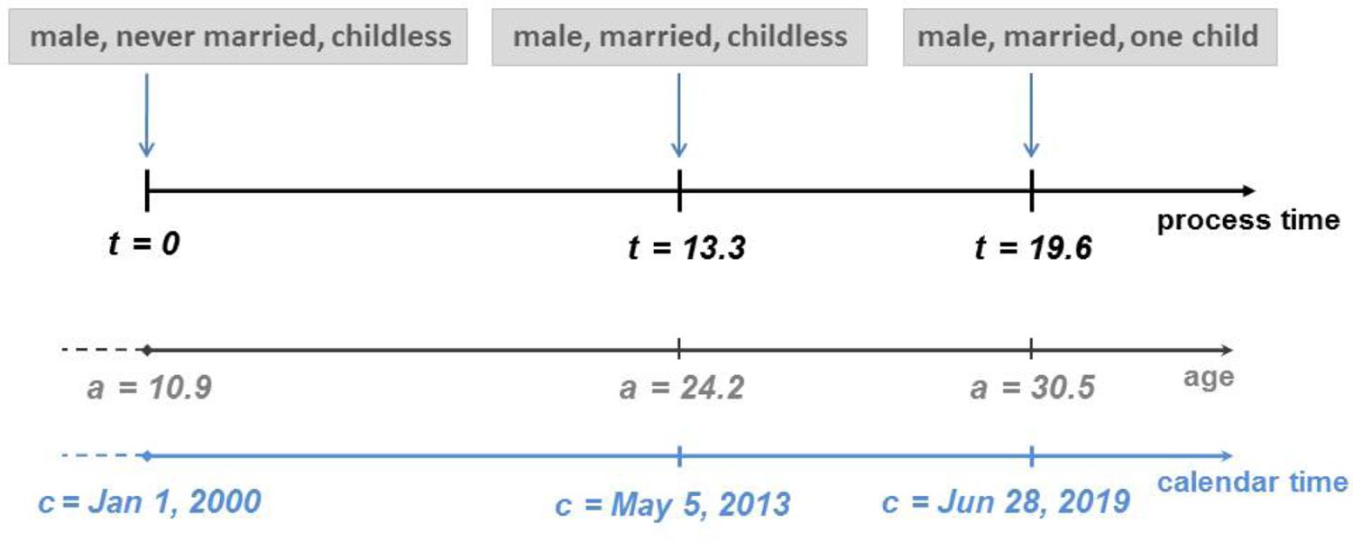
Sketch of a life-course of a male who is part of the initial population on January 1, 2000. At this time he is a = 10.9 years old, never married, and childless. On May 5, 2013, 13.3 years after he had entered the virtual population, he marries; and after 19.6 years he becomes father for the first time.

For many situations, it is feasible to assume that the propensity of an individual to change his/her current state depends only on his/her age, and possibly also on the calendar time. This applies, for example, to first birth events. However, some applications require the consideration of an additional third time scale: namely, the amount of time an individual has already spent in the current state. For example, the divorce risk strongly depends on the amount of time that has elapsed since the wedding (Becker et al., 1977; Diekmann & Schmidheiny, 2008) while the propensity to give birth to a second child depends on the amount of time that has elapsed since the delivery of the first child (Neyer & Andersson, 2008). To meet this need, the MicSim package allows life-course transitions hinging on age, calendar time, and also on the time already spent in a state. If life-course transitions are determined to depend on age or on age and calendar time, Z(t) can be described by a non-homogeneous continuous-time Markov process. If the user also assumes a dependence on the “time that has elapsed since the last event,” a non-homogeneous semi-Markov process must be used instead (Monteiro et al., 2006). Transition rates describing the propensity to leave a state to enter another one are the key quantities of the kind of stochastic processes. Once they are known, one can compute the distribution functions of the waiting times in the distinct states of the state space, and thus random variates of (latent) waiting times to next events. Since the microsimulation model implemented in the MicSim package specifies life-courses as sequences of waiting times to the next event, these random waiting time variates are its building blocks. A comprehensive and detailed documentation of how to derive from transition rates waiting time variates and from them synthetic life-courses is given in great detail elsewhere, see, for example, Zinn (2011, Chapter 2.3). We refer the interested reader to this literature.

In the MicSim package, life-courses can be described using non-homogeneous continuous-time Markov processes and non-homogeneous semi-Markov processes in combination; that is, different types of life-course events can be specified by either one or the other model type. For example, as a next event, a married woman with one child might either experience a divorce or become mother again or die. A different stochastic model might apply to each of these events. Concretely, the divorce risk and the propensity of giving birth to a second child can properly be explained by non-homogeneous semi-Markov processes, whereas mortality can be mapped by a non-homogeneous continuous-time Markov process. Once the user has figured out for a specific application the best models to use, that information and the corresponding transition rates have to be entered into MicSim. The process for doing this is the topic of the next section.

Note that in MicSim the life-course of an individual is censored at simulation end date if simulation stop date has been reached before the individual has died or emigrated.

2.4.2 Specifying models for life-course events in MicSim

Before life-courses can be constructed, the transition pattern applied during simulation has to be detailed. In other words, the user has to provide MicSim with information about the events that should be considered. The MicSim package requires two types of information: first, for all events and time scales along which dependency is assumed, functions of transition rates have to be defined; and, second, a transition matrix has to be determined which indicates when which transition rates function applies.

Transition rates functions

All of the transition rates have to be provided in form of R functions; that is, for each transition considered during the simulation, the user has to specify a corresponding transition rates function. By convention, a transition rates function might apply to distinct types of events; for example, a function describing non-parity specific fertility rates applies to all parity-specific birth events. The naming of the transition rates functions is up to the user. Each transition rates function has to feature three numerical input arguments: age, calTime, and duration. Via age the age of an individual is provided, via calTime the calendar time is entered, and via duration the time that has been elapsed since the last transition is provided. Not all of the input parameters have to affect the result of the transition rates function (also only one or two input parameters can affect the result). The user can also specify that none of the input parameters affects the result of the transition rates function; that is, a transition rate can be defined as being constant. This depends on the stochastic model assumed for an event. If the rates are assumed to be independent of a specific time scale, the corresponding input argument can simply be ignored within the body of the function when determining the specific rate values. All of the input arguments have to be given in decimal years. It should be noted that the time elapsed is measured starting from the last change in the state variable affected; that is, if a transition rates function describes the propensity for a second birth, duration marks the time since the first birth. For example, the transition rates among women of giving birth to a second child could be assumed to follow the Hadwiger mixture model (Chandola et al., 1999):


R> fert2Rates <- function(age, calTime, duration){
+ b <- ifelse(calTime <= 2020, 6.0, 5.7)
+ c <- ifelse(calTime <= 2020, 32, 33)
+ rate <- (b / c) * (c / age) <sup>Λ</sup> (3 / 2) *
+ exp(- b <sup>Λ</sup> 2 * (c / age + age / c − 2))
+ rate[age <= 15 | age >= 45 | duration < 0.75] <- 0
+ return(rate)
+ }

Here, the transition rates to giving birth to a second child are defined such that they vary with age, calendar time, and the time elapsed since first birth. The function returns zero for a time period of 0.75 years after the first birth. Thus, it accounts for the time range when a woman is pregnant. Furthermore, the function fert2Rates defines that women younger than age 16 and older than age 44 cannot have a (further) child. To describe age- and calendar time-dependent mortality rates, we might use the Gompertz model, parameterized to vary with age, and for periods before the year 2020 and after that year. Since we measure the duration in a state starting from the last change in the state variable affected, any kind of duration dependence of the mortality process is already described by its age dependence. (In other words, age is the time already spent in the “alive state.”) Hence, the duration argument is not used when computing the mortality rates.


R> mortRates <- function(age, calTime, duration){
+ a <- 0.00003
+ b <- ifelse(calTime <= 2020, 0.1, 0.097)
+ rate <- a * exp(b * age)
+ return(rate)
+ }

To ensure viable simulation results, every transition rates function has to return feasible values, at least for the considered simulation horizon and for all ages ranging from zero to the maximum age specified. All of the transition rates functions specified have to handle vectors of input values.⁹ This is the case with most R functions, and should not cause any problems. A special feature of the MicSim package is that it is able to handle deterministic events which occur with the probability of one at predetermined (whole numbered) ages, calendar years, or duration spans. This is achieved by setting the accordant transition rate(s) to infinity. For instance, we determine that every child will certainly enter elementary school in the year when he/she turns seven years old. The respective transition rates function may then be defined as follows:


R> noToLowEduRates <- function(age, calTime, duration){
+ rate <- ifelse(age == 7, Inf, 0)
+ return(rate)
+ }

This function returns infinity for age seven, and zero otherwise. It does not depend on calendar time nor on the time elapsed in a state. If for one specific transition deterministic events have been defined to happen at several points in time (e.g., at age seven, age 20, and age 50), MicSim chooses the earliest of these events.

Transition matrix

After having defined transition rates functions for all events of interest, the user has to specify the transition pattern to which they apply. For this purpose, a transition matrix (denoted as transitionMatrix) has to be constructed which indicates the possible (and impossible) transitions between the states of the state space, as well as the names of the functions determining the respective events. The transition matrix consists of as many rows as the state space contains states, and of as many columns as the state space contains states, plus the number of absorbing states defined. Since dying is a competing risk to which all individuals are always exposed, it mandatorily comprises a minimum of one absorbing state (namely, “dead”), and a maximum of two absorbing states if “emigrated” is also considered. By definition, the rows of the transition matrix correspond to the states in which the transitions start, and the columns correspond to the states in which the transitions end. We illustrate the design of the transition matrix by means of our simple mortality example that includes only two state variables: sex and mortality. The accordant state space is defined as


R> sex <- c("m", "f")
R> stateSpace <- sex R> attr(stateSpace, "name") <- "sex"
R> absStates <- "dead"

Here, we determine that transitions are only possible to dead; that is, this example does not include any transitions between nonabsorbing states. The MicSim package contains the function buildTransitionMatrix, which helps the user construct the transition matrix. The function has three input arguments: allTransitions, absTransitions, and stateSpace. Obviously, the argument stateSpace comprises the nonabsorbing states of the state space of the microsimulation application. Its definition is extensively described in Section 2.1. The input matrix allTransitions consists of all of the possible transitions between values of state variables (which are not “dead” or “emigrated”) in the first column and in the second column it contains the names of the functions that define the corresponding transition rates. Likewise, the matrix absTransitions contains the names of the absorbing states which individuals are exposed to (i.e., “dead” for being dead or “rest” for emigrated) in the first column, and the names of the functions defining the corresponding transition rates in the second column. By means of buildTransitionMatrix, we can define the transition matrix of our simple example as follows.


R> absTransitions <- c("dead", "mortRates")
R> transitionMatrix <- buildTransitionMatrix(
+ allTransitions = NULL, absTransitions =
+ absTransitions, stateSpace = stateSpace)

Here, allTransitions is set to NULL because our simple example only includes transitions to “dead.” To absTransitions a vector is assigned which indicates that the (user-defined) function mortRates describes all of the mortality rates. Hence, in sum, we yield the subsequent transition matrix. (The character “0” marks impossible transitions.)

m f dead
m "0" "0" "mortRates"
f "0" "0" "mortRates"

For further illustration, let us consider a slightly more complicated example involving the three state variables sex, being partnered, and mortality. Being partnered takes the two values “being alone” (labeled as “A”) and “being partnered” (labeled as “P”). The corresponding state space is given by


R> sex <- c("m", "f")
R> partnered <- c("A", "P")
R> stateSpace <- expand.grid(sex = sex, partnered =
+ partnered)
R> absStates <- "dead"

We are interested in partnership formation and dissolution events; that is, in the transitions between “A” and “P.” Furthermore, all of the individuals are always exposed to the risk of dying. In this example, for all of the events we assume distinct transition rates for females and males. We construct the corresponding transition matrix using the function buildTransitionMatrix. The specification of stateSpace is as described. As was already stated, the matrix allTransitions determines the transitions originating from nonabsorbing states in its first column, and the corresponding transition rates functions in its second column. Each element of its first column has to be of the form “X->Y,” with “X” indicating the starting value of a transition and “Y” indicating the arrival value. The character -> is the placeholder defined as marking a transition. For example, “A” describes the starting value of a partnership formation event and “P” describes its arrival value. (Clearly, all of the value labels used have to be identical to the value labels of the state variables specifying the simulation model.) In the example considered, we assume that all of the transition rates depend on the value of another state variable; namely, on the value of sex. The buildTransitionMatrix function allows us to use such a setting in a straightforward way, as it facilitates the specification of transitions that depend on one or more state variables. Therefore, the starting value and the arrival value of a transition have to be specified as a combination of the considered attributes, separated by a forward slash and in accordance with the ordering of the state variables in the state space. For example, “f/A->f/P” describes a female specific transition from “A” to “P.” For absorbing states, a prefix indicates the attributes on which a transition is assumed to depend (also separated by a forward slash), for example, “f/dead” and “m/dead” describe gender-specific mortality transitions. Thus, the input matrices allTransitions and absTransitions can be defined as follows:


R> trMatrix_f <- cbind(c("f/A->f/P", "f/P->f/A"),
+ c("rates1", "rates2"))
R> trMatrix_m <- cbind(c("m/A->m/P", "m/P->m/A"),
+ c("rates3", "rates4"))
R> allTransitions <- rbind(trMatrix_f, trMatrix_m)
R> absTransitions <- rbind(c("f/dead", "mortRates_f"),
+ c("m/dead", "mortRates_m"))

Here, rates1, rates2, rates3, and rates4 indicate (where applicable) the transition rate functions related to partnership formation and dissolution, and mortRates_f and mortRates_m give gender-specific mortality rates. Hence, for allTransitions we obtain


[1,] "f/A->f/P" "rates1"
[2,] "f/P->f/A" "rates2"
[3,] "m/A->m/P" "rates3"
[4,] "m/P->m/A" "rates4"

and for absTransitions we get


[,1] [,2]
[1,] "f/dead" "mortRates_f"
[2,] "m/dead" "mortRates_m"

All in all, we obtain the corresponding transition matrix by


R> transitionMatrix <- buildTransitionMatrix(
+ allTransitions = allTransitions, absTransitions =
+ absTransitions, stateSpace = stateSpace)

that is, the transitionMatrix is


m/A f/A m/P f/P dead
m/A "0" "0" "rates3" "0" "mortRates_m"
f/A "0" "0" "0" "rates1" "mortRates_f"
m/P "rates4" "0" "0" "0" "mortRates_m"
f/P "0" "rates2" "0" "0" "mortRates_f"

3. Special features of micSim

The base population, the transition matrix, and the corresponding transition rates functions are mandatory ingredients for conducting a microsimulation run. The inclusion of migration, the creation of newborns during the simulation, and enrollment in elementary school is optional. This section deals with the specification of these extra options

3.1 Simulating offspring

In the MicSim package, the user decides whether female fertility results in offspring. For this purpose, an accordant vector (denoted as fertTr) has to be specified marking all of the transitions triggering a childbirth event during simulation; that is, the creation of a new individual. Obviously, such transitions have to be in accordance with the state space and the previously defined transition pattern. Consider, for example, the following state space comprising sex and fertility:


R> sex <- "f"
R> fert <- c("0", "1+")
R> stateSpace <- expand.grid(sex = sex, fert = fert)
R> absStates <- "dead"

The state variable “sex” takes only the value female (labeled “f”), and the state variable fert maps being childless (labeled “0”) and being mother (labeled “1+”). The corresponding transition matrix is defined as:


R> allTransitions <- cbind(c("0->1+", "1+->1+"),
+ c("fertRates1", "fertRates2"))
R> absTransitions <- c("dead", "mortRates")
R> transitionMatrix <- buildTransitionMatrix(
+ allTransitions = allTransitions, absTransitions =
+ absTransitions, stateSpace = stateSpace)

On that, we define that during simulation transitions of the type “0→1+” and “1+→1+” imply newborns.


R> fertTr <- c("0->1+","1+->1+")

Once the microsimulation yields a newborn, he/she has to be assigned to the state space. The process MicSim employs to do this is detailed in Section 2.3. Ultimately, it is left to the user to determine the possible initial states of newborns and their occurrence probabilities (initStates and initStatesProb). As a default, the MicSim package does not account for any offspring; i.e., fertTr = c(), initStates = c(), initStatesProb = c().

3.2 Enrolment in elementary school

If the state space includes educational achievement and if individuals of the relevant age are simulated, it may be necessary to model the enrolment of children in elementary school. The MicSim package is able to take into account enrolment events that take place on a general enrolment date (denoted as dateSchoolEnrol) of a particular year. For this purpose, first a state variable defining educational attainment has to be created. Then, labels of possible values have to be defined, with “no” describing no education and “low” describing elementary education. The general enrolment date is set via dateSchoolEnrol using a string of the form “month/day,” for example, “09/13” for September 13. The default setting is “09/01.” Finally, the transition function determining the transition rate for the respective enrolment event has to be defined to return Inf for the age x at which children should be enrolled (e.g., at age seven), and zero otherwise. In this way, an event “school enrolment on dateSchoolEnrol of the year in which a child turns x years old” is determined.


R> sex <- c("m", "f")
R> edu <- c("no", "low")
R> stateSpace <- expand.grid(sex = sex, edu = edu)
R> absStates <- "dead"


R> dateSchoolEnrol <- "09/01"
R> noToLowEduRates <- function(age, calTime, duration){
+ rate <- ifelse(age == 7, Inf, 0)
+ return(rate)
+ }


R> allTransitions <- matrix(c("no->low",
+ "noToLowEduRates"), nrow = 1)
R> absTransitions <- c("dead", "mortRates")
R> transitionMatrix <- buildTransitionMatrix(
+ allTransitions = allTransitions, absTransitions =
absTransitions, stateSpace = stateSpace)

Generally, it is completely up to the user how to define changes in the educational achievement. As described, enrolment to elementary school can be modelled to happen on a pre-defined general enrolment date at a certain age. Alternatively, it can be modelled to happen, for example, in a certain (whole numbered) year or even completely at random. In the latter cases, the user has simply to choose labels others than “no” and “low” to describe enrolment to elementary school, set dateSchoolEnrol=c(), and to determine the related transition rates functions accordingly (cp. Section 2.4.2).

3.3 Following migrants

The MicSim package also offers the option of allowing immigrants to enter the virtual population during simulation. In Section 2.3, we describe in detail how migration data have to be prepared so that MicSim can process them. After migrants have entered the virtual population, the user might be interested in following them. The generic model of MicSim can easily cope with such a demand. The user simply has to specify a state variable called “being a migrant,” with a value that indicates whether an individual is a migrant. When entering the virtual population, the respective state value is then assigned according to the migration status of an individual. For example, the state (male, divorced, childless, high education, being migrant) describes a childless, divorced man with a high level of education who is flagged as being a migrant when entering the virtual population by immigration. Once a migrant is assumed to be assimilated into the population of immigration his/her status changes to “not being a migrant.” For this purpose, only an accordant transition rate has to be defined. For example, five years after migration, the probability that a migrant will behave like a native is assumed to be one. By its very nature, such an event is similar to an enrolment event into elementary school (cp. Section 3.2), and thus has to be defined accordingly: namely, a transition rate is defined as being equal to infinity for a duration of stay that is five years or longer. An excerpt of the related source code is given in the subsequent. The whole example can be found in the appendix.


R> migrant <- c("mig", "notMig")
R> stateSpace <- expand.grid(sex = sex, migrant = migrant)
R> migToNotMigRates <- function(age, calTime, duration){
+ rate <- ifelse(duration >= 5, Inf, 0)
+ return(rate)
+ }
R> allTransitions <- matrix(c("mig->notMig",
+ "migToNotMigRates"), nrow = 1)

4. Conducting microsimulation and output

After having defined

the base population initPop,
the maximum age maxAge,
the simulation horizon simHorizon,
the state space of nonabsorbing states stateSpace,
the set of absorbing states absStates, and
the transition rates functions and the accordant transition pattern (reported by means of the transition matrix; transitionMatrix),

and, optionally also

data on migrants immigrPop,
transitions leading to offspring fertTr, and
a general date of enrolment to elementary school dateSchoolEnrol,

the MicSim package has been provided with all of the information required to perform a microsimulation run. For this purpose, the package offers two functions. The function micSim conducts microsimulation using one single CPU core. In terms of run times, this is not a very performant solution, especially today when most computers are equipped with CPUs with more than one core. The function micSimParallel performs microsimulation making use of as many cores as the user specifies. Of course, the number is restricted by the maximum number of cores a computer (or a computer cluster) has. When conducting any kind of simulation, one should always pay special attention to the pseudo random number generator (PRNG). By default, R uses the Mersenne Twister, which is based on a matrix linear recurrence over a finite binary field (Matsumoto & Nishimura, 1997). The MicSim package relies on the positive qualities of the Mersenne Twister, and applies it for microsimulation. To ensure that the results are replicable and are therefore reasonable, the user should always assign a seed to each PRNG representation used. Thus, for each core accessed, MicSim asks for a seed. When running the microsimulation on a single core, we define the seed by means of the set.seed function before calling the actual microsimulation function micSim.


R> set.seed(234)
R> pop <- micSim(initPop = initPop, transitionMatrix =
+ transitionMatrix, absStates = absStates, maxAge =
+ maxAge, simHorizon = simHorizon)

Alternatively, if immigration, offspring born during the simulation, and enrolment in elementary school are also considered, the following command conducts a single-core microsimulation run:


R> set.seed(234)
R> pop <- micSim(initPop = initPop, immigrPop = immigrPop,
+ transitionMatrix = transitionMatrix, absStates =
+ absStates, initStates = initStates, initStatesProb =
+ initStatesProb, maxAge = maxAge, simHorizon =
+ simHorizon, fertTr = fertTr, dateSchoolEnrol =
+ dateSchoolEnrol)

In the multicore specification, we enter a set of seeds via the input arguments of micSimParallel. An accordant example is given in the appendix.

The output object pop of micSim and micSimParallel is a data frame that contains the whole synthetic population considered during the simulation, including all of the events generated; that is, the pop object contains as many rows as there are transitions performed by the individuals of the virtual population. (“Entering the virtual population” is also considered as an event.) For the example focusing on individual behaviour concerning changes in marital status, educational attainment, and fertility status (The accordant state space is described in Section 2.3.) and the simulation horizon from January 1, 2014, to December, 31, 2050, we get the following output:

birthDate

initState

From

transitionTime

transitionAge

25/Feb/1968

f/3+/NM/med

f/3+/M/med

29/Jul/2018

50.43

25/Feb/1968

f/3+/NM/med

f/3+/M/med

dead

30/Apr/2049

81.18

09/Jun/1984

m/3+/M/high

m/3+/D/high

07/Apr/2023

38.83

09/Jun/1984

m/3+/M/high

m/3+/D/high

m/3+/M/high

21/Feb/2024

39.70

06/0ct/1989

f/2/D/med

f/3+/D/med

13/Jul/2015

25.77

06/0ct/1989

f/2/D/med

f/3+/D/med

29/Mar/2020

30.48

06/0ct/1989

f/2/D/med

f/3+/D/med

05/Sep/2020

30.92

06/0ct/1989

f/2/D/med

f/3+/D/med

25/Jan/2021

31.31

15299

06/Dec/2050

m/0/NM/no

<NA>

15300

23/Dec/2050

f/0/NM/no

<NA>

The column ID gives the unique numerical person identifiers, the column birthDate gives the birth dates of the individuals, and the column initState gives the states the individuals were in when they entered the virtual population. The columns From and To mark the transitions the individuals experienced during the simulation. From gives the states of origin and To gives the states of destination. The columns transitionTime and transitionAge document the corresponding transition dates and ages. In the example given, the individual with ID=1 is a female born on February, 25, 1968, who enters the virtual population by being part of the base population. At simulation starting time she is a never married woman with a lower secondary education and mother of three or more children. She marries on July 29, 2018 at age 50.43. On April 30, 2049 at age 81.18 she dies. The two individuals shown at the end of the example are born during the simulation; namely, on December 6, 2050 and on December 23, 2050. Apart from their birth, no further events are simulated up to the end point of the simulation, as indicated by the <NA> and NA entries in the respective lines. Generally, micSim and micSimParallel return all of the birth dates and the transition dates in the form of chron objects.

To ease further processing, the MicSim package provides a function that reshapes the microsimulation output into a long format that might be more familiar to people working with event data. That function, called convertToLongFormat, transforms the microsimulation output into a dataset with one row for each episode which an individual experiences.¹⁰ The function convertToLongFormat contains two input arguments: the output object of micSim or micSimParallel and an indicator variable marking whether the simulation model considered immigration (the default setting is “no immigration considered”).


R> convertToLongFormat(pop, migr = TRUE)

By means of the example given above, we detail the output of the function convertToLongFormat.

birthDate

Tstart

Tstop

status Entry

status Exit

Episode

sex

fert

marital

edu

25/Feb/1968

01/Jan/2014

29/Jul/2018

NM->M

med

25/Feb/1968

29/Jul/2018

30/Apr/2049

dead

med

09/Jun/1984

01/Jan/2014

07/Apr/2023

M->D

high

09/Jun/1984

07/Apr/2023

21/Feb/2024

D->M

high

09/Jun/1984

21/Feb/2024

31/Dec/2050

cens

high

06/Oct/1989

01/Jan/2014

13/Jul/2015

2->3+

med

06/Oct/1989

13/Jul/2015

29/Mar/2020

3+->3+

med

06/Oct/1989

29/Mar/2020

05/Sep/2020

3+->3+

med

15299

06/Dec/2050

<NA>

31/Dec/2050

cens

15300

23/Dec/2050

<NA>

31/Dec/2050

cens

The first column gives the unique numerical person identifier ID and the second column gives the birth date of an individual. The variables Tstart and Tstop mark the start and the end dates of episodes. The column statusEntry specifies whether the entry into an episode has been observed. The value “1” marks an observed entry, and the value “0” marks a left-truncated episode. Likewise, the column statusExit specifies whether the episode was completed by a transition between two states or by right-censoring. Value “1” indicates a transition and value “0” indicates a censoring event. The column OD identifies the transition which completed an episode. Here, right-censoring is marked by “cens.” The column ns gives the number of episodes an individual has passed and the column Episode enumerates these episodes. The last columns of the data frame contain for each individual and episode the values of the state variables during that episode, such as “sex,” or “education.”

5. Conclusion

The R package MicSim performs continuous-time microsimulations for population projection. Its key ingredients are the virtual population and a stochastic model describing life-course dynamics. The virtual population maps the composition and the development of the population under study along simulation time. To each individual who is part of the virtual population, a set of demographically relevant attributes is assigned. These attributes may change along the simulation time span. To describe life-course dynamics, stochastic models are usually applied. The MicSim package implements two classes of stochastic models: non-homogeneous continuous-time Markov processes and non-homogeneous semi-Markov processes. The first class of models specifies life-course events over age and calendar time. The second class of models also postulate duration dependence; that is, it assumes that the propensity of an individual to change his/her current set of attributes may depend not only on his/her age and on calendar time, but also on the amount of time elapsed since a last transition. Thus, the MicSim package is able to cover a wide range of situations relevant for demographic population projections. A further useful feature of the MicSim package is its ability to deal with deterministic events. In other words, the package allows the user to specify that certain events will occur with a probability of one. A relevant example is the enrolment of children in elementary school in the year in which they turn seven years old. Furthermore, due to the generic structure of the microsimulation model being implemented, the MicSim package allows users to follow migrants once they have entered the virtual population. All in all, we find that the MicSim package is able to conduct meaningful population projections at a very fine-grained level from a relatively low level entry point. This article provides excerpts of examples that illustrate its applicability. The full specification of the examples given can be found on the help pages of the package.

Clearly, the work on the MicSim package is not completed, and there are several issues that still need to be addressed. One challenge lies in taking into account the amount of time individuals have already spent in their initial states when entering the virtual population. This is of special importance if semi-Markov processes are used to describe life-course dynamics. Ignoring the time already spent in the initial states might cause distorted first event times. In particular, members of the base population and migrants are affected by this problem. In its current version, the MicSim package does not ask for the time spans members of the base population and migrants have spent in their initial states. Thus, this kind of information is not accessible for further processing. This issue is related to another problem: namely, that of which time point should be used as a reference point for duration measurement. Currently, the MicSim package measures the length of duration starting from the last change of the affected state variable. While this might make sense with regard to birth intervals and gestation gaps, it could be problematic with regard to divorce events. For example, we know that the divorce risk depends not only on the time elapsed since the wedding, but also on the time elapsed since the last birth event (if there was one). We are currently extending the MicSim package to tackle these issues: First, we are broadening the definition of the base population and the definition of the set of immigrants so that the time already spent in the initial states can be documented. In addition, we will provide the user with the opportunity to decide the reference point of the duration measurement for each event separately.

The R environment provides a huge set of visualization tools. However, the MicSim package currently does not make use of this potential and does not offer any plotting option. As the MicSim package relies on a generic microsimulation model, the simulation outcome might be of any type, and tailor-made plotting functions are hard to specify. We therefore argue that the user will know best how he/she wants the simulation output of a specific application to be visualized. Furthermore, we recommend the use of existing visualization devices provided by other related R packages. For example, the Biograph package (Willekens, 2013) makes it possible to plot life histories in Lexis diagrams and to generate state occupation diagrams, while the TraMineR package facilitates the visualization of state and event sequences (Gabadinho et al., 2014). Nevertheless, we are currently working on a set of plotting functions that apply to particular situations, such as population pyramids that refer to distinct time points.

The presented microsimulation model can be extended in other directions, as well. Parental characteristics and behaviour might be modelled to influence children’s characteristics and behaviour. Marriage markets can be included, with couples and household entities being modelled and simulated. Furthermore, macro components such as macroeconomic indicators might be considered and spatial patterns may be added. However, including a large number of potential influencing factors in a microsimulation model is generally difficult, as causal relationships might be disturbed and even distorted. Hence, while it is possible to add some of the functionality outlined above to the MicSim package, doing so would require very careful reasoning, and thus remains an issue for further research and software versions.

Footnotes

1.

The MicSim package is licensed under the terms of the GPLv2.

2.

For example, a single-core run of the microsimulation application on studying living arrangement, educational carrier and fertility transitions which we describe in Section 2 lasts ca. 400 seconds on a desktop workstation equipped with Intel(R) Core(TM)i7, CPU 2.80GHz, 8GB RAM, under Windows 7 (64bit), MicSim version 1.0.6 and R version 3.0.1. Running the same application with six cores lasts ca. 65 seconds. This is an approximate run time reduction by factor 6. By contrast, the Mic-Core needs ca. 6 seconds to perform a comparable simulation run, which means a further run time reduction by approximately factor 10.

3.

To access the help page of the micSim function start R. Then, instruct R to download the packages MicSim, chron, snowfall, and rlecuyer from the R package database CRAN. After R has finished this task, enter the command library(MicSim) into the R input window (completed by pressing ENTER). The MicSim package is loaded. Subsequently, enter the command ?micSim (again completed by pressing ENTER). Now the help page of the micSim function of the MicSim package opens.

4.

The source code can simply be copied into the R input window and the examples instantly being performed.

5.

If the user really does not want to incorporate transitions to “dead,” this can be achieved by setting the mortality risk to zero; see also Section 2.4.3.

6.

If other states than “dead” or “emigrated” should be defined as not being left again, their transition rates have to be set to zero; see also Section 2.4.3.

7.

Here, we have to be careful to ensure that R does not convert strings into factors when constructing the data frame, by using the command stringsAsFactors = FALSE. This type of conversion causes problems when the microsimulation is run.

8.

In the recent version of the MicSim package, all individuals are modelled and simulated as being completely independent of each other. Consequently, for example, child characteristics cannot be made dependent on mother characteristics. The only exception is the event of childbirth. If specified by the user, such an event leads to the creation of a new individual, see Section 3.1. The assumption of independent life-courses is a clear limitation, which surely has to be changed in an upcoming version of the MicSim package. However, the source code of all functions implemented in the package can be read by the user and thus be adapted to meet own needs. The user has simply to enter the name of the function of interest into the R input window, for example, micSim. Then, the related source code is printed. Admittedly, adapting source code requires a deeper knowledge of R programming.

9.

The MicSim package solves the integrated hazard which is an essential part of the distribution function of a latent waiting time in a state by means of R’s integrate function. This function requires the functions to integrate to be able to deal with vectors of input values.

10.

The MicSim package also provides the function convertToWideFormat reshaping microsimulation output into wide format. In wide format, the data comprises for each episode which an individual experiences additional column entries.

Following migrants: an example

The MicSim package allows following migrants and integrating them into the native population after some time, for example, after five years. The source code of an accordant example is given in the subsequent.

First, we define the simulation horizon and the state space comprising besides “dead” the state variables “sex” and “migrant”. The migrant variable has two values: “being migrant” (mig) and “not being migrant” (notMig).


R> simHorizon <- setSimHorizon(startDate="01/01/2000",
+ endDate="31/12/2020")
R> sex <- c("m", "f")
R> migrant <- c("mig", "notMig")
R> stateSpace <- expand.grid(sex = sex, migrant = migrant)
R> absStates <- "dead"

Then, we construct a base population with five individuals.


R> dts <- c("31/12/1930", "03/04/1999", "15/10/1956",
+ "11/11/1991", "01/01/1965")
R> birthDates <- chron(dates = dts, format = c(dates =
+ "d/m/Y"))
R> initStates <- c("f/notMig", "m/notMig", "f/notMig",
+ "m/notMig", "m/notMig")
R> initPop <- data.frame(ID = 1:5, birthDate = birthDates,
+ initState = initStates, stringsAsFactors = FALSE)

We create five migrants entering the virtual population at June 6, 2001.


R> # Defining a set of migrants; M=5 R> IMdts <- rep(c("6/6/2001"), 5)
R> immigrDates <- chron(dates = IMdts, format = c(dates =
+ "d/m/Y"))
R> IMinitStates <- c("f/mig", "m/mig", "f/mig", "m/mig",
+ "m/mig")
R> immigrPop <- data.frame(ID = 6:10, immigrDate =
+ immigrDates, birthDate = birthDates, immigrInitState =
+ IMinitStates, stringsAsFactors = FALSE)

The transition rate for experiencing a transition from “being migrant” to “not being migrant” is set to zero during the first five years after migration and set to infinity after that time.


# Defining a transition rate for becoming a nonmigrant R> migToNotMigRates <- function(age, calTime, duration){
+ rate <- ifelse(duration >= 5, Inf, 0)
+ return(rate)
+ }

We use the Gompertz model to describe mortality rates.


R> mortRates <- function(age, calTime, duration){
+ a <- 0.00003
+ b <- ifelse(calTime <= 2020, 0.1, 0.097)
+ rate <- a * exp(b * age)
+ return(rate)
+ }

The transition matrix determines two possible events, namely the transition from “being migrant” to “not being migrant” and dying.


R> allTransitions <- matrix(c("mig->notMig",
+ "migToNotMigRates"), nrow = 1)
R> absTransitions <- c("dead", "mortRates")
R> transitionMatrix <- buildTransitionMatrix(
+ allTransitions = allTransitions, absTransitions =
+ absTransitions, stateSpace = stateSpace)

After having defined all of the ingredients required, we are ready to conduct a microsimulation run.


R> set.seed(234)
R> pop <- micSim(initPop=initPop, immigrPop=immigrPop,
+ transitionMatrix=transitionMatrix,
+ absStates=absStates, maxAge=maxAge,
+ simHorizon=simHorizon)

Parallel execution via micSimParallel

For a simple setting (without considering immigration, offspring born during the simulation, and enrolment in elementary school), a parallel execution on, for example, five cores can be performed by:


R> cores <- 5
R> seeds <- c(1233, 1245, 1234, 5, 2)
R> pop <- micSimParallel(initPop = initPop, transitionMatrix + = transitionMatrix, absStates = absStates, maxAge =
+ maxAge, simHorizon = simHorizon, cores = cores, seeds
+ = seeds)

Here, the number of cores to be accessed and the related set of seeds are given to micSimParallel via its input arguments cores and seeds. When accounting in addition for migration, offspring born during the simulation, and enrolment in elementary school, the following command is used:


R> cores <- 5
R> seeds <- c(1233, 1245, 1234, 5, 2)
R> pop <- micSimParallel(initPop = initPop, immigrPop =
+ immigrPop, transitionMatrix = transitionMatrix,
+ absStates = absStates, initStates = initStates,
+ initStatesProb = initStatesProb, maxAge = maxAge,
+ simHorizon = simHorizon, fertTr = fertTr,
+ dateSchoolEnrol = dateSchoolEnrol, cores = cores, seeds
+ = seeds)

References

1
Survival and event history analysis: A process point of view
(2008)
Springer.
- Google Scholar
2
Multi-state models for event history analysis
1. P Andersen
2. N Keiding
(2002)
Statistical Methods in Medical Research 11:91–115.
- Google Scholar
3
An economic analysis of marital instability
(1977)
The Journal of Political Economy 85:1141–1187.
- Google Scholar
4
Event history analysis
(1989)
Lawrence Erlbaum Associates.
- Google Scholar
5
The log-logistic rate model: Two generalizations with an application to demographic data
1. J Brüderle
2. A Diekmann
(1995)
Sociological Methods & Research 24:158–186.
- Google Scholar
6
Recent European fertility patterns: Fitting curves to ‘distorted’ distributions
(1999)
Population Studies 53:317–329.
- Google Scholar
7
The intergenerational transmission of divorce: A fifteen-country study with the Fertility and Family Survey (ETH Zurich Sociology Working Papers No. 4)
1. A Diekmann
2. K Schmidheiny
(2008)
ETH Zurich, Chair of Sociology.
- Google Scholar
8
TraMineR: Trajectory miner: A toolbox for exploring and rendering sequence data [Computer software manual]
(2014)
TraMineR: Trajectory miner: A toolbox for exploring and rendering sequence data [Computer software manual], http://cran.r-project.org/package-TraMineR, (R package version 1.8.8).
- Google Scholar
9
Discrete-time and continuous-time approaches to dynamic microsimulation (reconsidered) (Tech. Rep.)
1. H Galler
(1997)
University of Canberra: NATSEM, National Centre for Social and Economic Modelling, University of Canberra.
- Google Scholar
10
Description of the microsimulation model (Technical report, MicMac project)
1. J Gampe
2. S Zinn
(2007)
Rostock: MPIDR.
- Google Scholar
11
JAMES II: Extending, using, and experiments
1. J Himmelspach
(2012)
208–210, Proceedings of the 5th International ICST Conference on Simulation Tools and Techniques, ICST, Brussels, Belgium, Belgium, ICST (Institute for Computer Sciences, Social-Informatics and Telecommunications Engineering).
- Google Scholar
12
Multi-state models: A review
1. P Hougaard
(1999)
Lifetime Data Analysis 5:239–264.
- Google Scholar
13
Markov processes for stochastic modeling
1. M Kijima
(1997)
167–241, Continuous-time Markov chains, Markov processes for stochastic modeling, Chapman & Hall.
- Google Scholar
14
Simulation modeling and analysis
1. A Law
2. W Kelton
(2000)
437–495, Generating random variates, Simulation modeling and analysis, Mc Graw Hill Higher Education.
- Google Scholar
15
jamsim: Java & R based microsimulation
1. O Mannion
(2014)
16
Jamsim: A microsimulation modelling policy tool
1. O Mannion
2. R Lay-Yee
3. W Wrapson
4. P Davis
5. J Pearson
(2012)
Journal of Artificial Societies and Social Simulation 15:8.
- Google Scholar
17
Mersenne twister: A 623-dimensionally equidistributed uniform pseudo-random number generator
1. M Matsumoto
2. T Nishimura
(1997)
Transactions on Modeling and Computer Simulation: Special issue on uniform random number generation 8:3–30.
- Google Scholar
18
Event history analysis in life course research
1. K Mayer
2. N Tuma
(editors) (1990)
University of Wisconsin Press.
- Google Scholar
19
Non-parametric estimation for non-homogeneous semi-Markov processes: an application to credit risk
(2006)
Tinbergen Institute.
- Google Scholar
20
Consequences of family policies on childbearing behavior: Effects or artifacts?
1. G Neyer
2. G Andersson
(2008)
Population and Development Review 34:699–724.
- Google Scholar
21
Parallel discrete-event simulation tool for population analysis
1. B Onggo
(2010)
Proceedings of the Operational Research Society Simulation Workshop 2010 (sw10).
- Google Scholar
22
μsik: A micro-kernel for parallel/distributed simulation systems
1. K Perumalla
(2005)
ACM/IEEE/SCS Workshop on Parallel and Distributed Simulation (pads).
- Google Scholar
23
R: A language and environment for statistical computing [Computer software manual]
1. R Development Core Team
(2013)
R: A language and environment for statistical computing [Computer software manual], Vienna, Austria.
24
Simulation and the Monte Carlo Method (2nd ed.)
1. R Rubinstein
2. D Kroese
(2008)
Wiley.
- Google Scholar
25
Modgen version 10.1.0: Developer's guide
1. Statistics Canada
(2011)
Modgen version 10.1.0: Developer's guide.
26
New frontiers in microsimulation modelling
1. F Willekens
(2009)
353–376, Continuous-time microsimulation in longitudinal analysis, New frontiers in microsimulation modelling, Ashgate, Farnham, Surrey, UK, (Book released during 2nd International Microsimulation Conference, Ottawa, June 2009).
- Google Scholar
27
Biograph: Explore life histories [Computer software manual], version (R package version 2.0.4)
1. F Willekens
(2013)
Biograph: Explore life histories [Computer software manual].
28
Simulation methods for analyzing continuous-time event-history models
1. D Wolf
(1986)
Sociological Methodology 16:283–308.
- Google Scholar
29
MicSim: Performing continuous-time microsimulation [Computer software manual], version (R package version 1.0.6)
1. S Zinn
(2014)
MicSim: Performing continuous-time microsimulation [Computer software manual].
30
Proceedings of the 2009 winter simulation conference
1. S Zinn
2. J Himmelspach
3. J Gampe
4. A Uhrmacher
5. MD Rossetti
6. RR Hill
7. B Johansson
8. A Dunkin
9. RG Ingalls
(2009)
Mic-core: A tool for microsimulation, Proceedings of the 2009 winter simulation conference, Piscataway, NJ, IEEE.
- Google Scholar
31
A continuous-time microsimulation and first steps towards a multi-level approach in demography
1. S Zinn
(2011)
PhD dissertation, Faculty of Information Science and Electrotechnics, University of Rostock, http://rosdok.unirostock.de/file/rosdok derivate0000004766/DissertationZinn2011.pdf.
- Google Scholar

Article and author information

Author details

Sabine Zinn
1. Max Planck Institute for Demographic Research Rostock, Germany
2. Leibniz Institute for Educational Trajectories Bamberg, Germany
For correspondence
sabine.zinn@lifbi.de

Acknowledgements

I have to acknowledge my gratitude to Frans Willekens who encouraged me and gave me the opportunity to develop and to work on the MicSim package. Furthermore, I am in debt to him and Anna Klabunde for fruitful discussions, a lot of helpful suggestions, and for revising first versions of this article. Moreover, I have to thank two anonymous referees for very helpful comments to improve the quality and the content of this article.

Publication history

Version of Record published: December 31, 2014 (version 1)

Copyright

This article is distributed under the terms of the Creative Commons Attribution License, which permits unrestricted use and redistribution provided that the original author and source are credited.

Download links

A two-part list of links to download the article, or parts of the article, in various formats.

Downloads (link to download the article as PDF)

Article PDF

Download citations (links to download the citations from this article in formats compatible with various reference manager tools)

BibTeX
RIS

Open citations (links to open the citations from this article in various online reference manager services)

Mendeley

Example state space: State variables and their corresponding values. (Value labels, subsequently used, are given in parentheses)

Author details

Sabine Zinn

For correspondence

Downloads (link to download the article as PDF)

Download citations (links to download the citations from this article in formats compatible with various reference manager tools)

Open citations (links to open the citations from this article in various online reference manager services)

Categories and tags