Spot on or way off? Validating results of the AVID microsimulation model retrospectively
- Deutsche Rentenversicherung Bund, Germany
Abstract
A well-known challenge for developers and users of dynamic microsimulation models is the question of credibility, the so-called black box problem. Several strategies have been proposed to validate models. They typically involve comparing the results of a simulation run to other suitable figures. This paper approaches the issue after a considerable time lag and uses empirical data for a retrospective comparison. The validation is concerned with the German AVID model, or more precisely, with the basic employment histories module of the model. The model uses survey data and process-generated data on app. 12 000 Germans to project future employment histories and future old age incomes. After seven years the original respondents were surveyed again so that it is possible to compare their simulated and empirical employment histories. Several aspects regarding desired properties of the simulation results and the characteristics of employment histories are discussed. They include global indicators like cross-sections on the aggregate level, cumulative values on the individual level, and structural indicators on the individual level. The results of the comparison are generally encouraging. On the aggregate and cumulative level there is a very good resemblance. Substantial deviations are only found on the individual, structural level: The empirical employment histories are much more continuous than the simulated ones. This overestimation of complexity can be explained by the developments in the time period used for the estimation of the model parameters, but it still leads to a general underestimation of social inequality in the simulation results.
1. Introduction
The motivation for this paper is the well-known perception of microsimulation models as black boxes. By their nature, the results of complex models and their underlying dynamics cannot be made completely transparent. Still, and especially in policy consulting, there is a need for information and for measures of credibility which can enhance the trust in a model. Commonly this trust is created by more or less extensive validation exercises.
The validation of complex models is not an easy task. It involves the question of what data the projection results should be compared to, and decisions on which areas should be taken into account and which indicators should be used. The approach taken in this paper is a retrospective one which compares the results of the projection with actual empirical data after a considerable time lag. The focus of this comparison is on employment histories, which form the core part of the AVID model.
Several indicators are considered. They cover different areas of interest when considering the quality of simulation results. Since the focus is on longitudinal, sequential data, it is not enough to consider cross-sections on an aggregate level. While they must of course fit with the comparison data, it is worthwhile to dig a bit deeper and consider indicators on the individual level as well. In the first part of the paper, different indicators are proposed, which shed light on different aspects such as the aggregate and individual level, and the content and structural dimensions of the employment histories.
However, the question of how well the model projected the actual developments is not the only one of interest in this paper. A second question, which is equally important to the validation exercise, is the question of how the differences between the two data sources can be explained, or, of what drives the results. Do we get these results because of something inherent in the model set-up, or should we point the finger at the base period used to estimate the parameters for the model?
This second question is especially important in the context of the German AVID model which used the ten years from 1992 to 2001 as base period. The 1990ies, following the collapse of the socialist Eastern bloc and the German reunification, have been very turbulent times, particularly in the Eastern part of the country. Period effects such as these pose a great challenge to model development since any projection has to rely on information derived from past events. But from a methodological point of view this is also a unique opportunity to see how the developments in the base period might affect the projection results.
The paper is structured as follows: Chapter 2 contains a brief discussion of previous research and introduces the AVID model. Then, a set of indicators is developed, which cover different aspects of the simulation. Lastly, the validation approach and data sources are explained. In chapter 3 the results are presented following the basic outline of the indicators introduced in chapter 2. A discussion highlights the most important results and puts them into perspective (Chapter 4), before Chapter 5 offers some concluding remarks.
2. Background
The validation of a dynamic microsimulation model typically consists of comparing the model results to other suitable figures. The idea is to see if the numbers fit and, especially if there are differences, to gain a better understanding of what drives the results (Morrison 2008: 12). While the model is still under construction it can be helpful to run it for a time in the past, i.e. the time period which the parameters are derived from. Another approach along these lines could be to divide the data in halves and use the parameters from the training set to reproduce the results in the comparison set. But “other suitable figures” could also be runs of the same model without certain modules or the results of a simple stylized model (Dekkers 2014).
It is apparent that the term validation is used for different actions and in different stages of the model development. Validation can be understood very broadly and comprehensively and then it can encompass many different activities with which the development team ensures that the model results are plausible and credible. Examples of this broad approach which also give a detailed description of different validation activities can be found in Morrison (2008) and Harding, Keegan and Kelly (2010).
The idea of a stylized model introduced by Dekkers (2014) has a much narrower understanding of validation which is closer to how the concept is used in this paper.1 Validation in this sense has less to do with model development and more with credibility, application and selling of the results. With this approach the validation exercise should provide a feeling for “how good the projection results are” and ideally provide the model with credibility. This paper shares the narrow definition of validation, but the model results are compared to empirical data, a retrospective approach also suggested by Li, O'Donoghue and Dekkers (2014). This unfortunately implies that the validation can only happen after a considerable time lag when the urgency of creating trust in the model’s results is less strong. But the advantage of this approach lies in the authenticity of the comparison data.
The three examples given above show that the setup of validation exercises can be very different. But they always have to fit with the aim and scope of the model and the indicators should reflect these as much as possible. The following section therefore provides some brief background information on the AVID dynamic microsimulation model. It then presents the aspects of the projection which are considered important and introduces the corresponding indicators. Lastly the approach is explained in more detail and the empirical data used for the retrospective validation is introduced.
2.1 The AVID model
The AVID dynamic microsimulation model was developed by ASKOS and TNS Infratest Sozialforschung for the German Federal Pension Insurance and the German Federal Ministry of Labour and Social Affairs (Heien, Kortmann & Schatz 2007). Its purpose is the projection of future pension entitlements in all German pension schemes, including occupational pension schemes and private provisions.
The current model is based on an earlier version (AVID 1996) and was developed between 2002 and 2007 (Roth, Stegmann & Bieber 2002). As no suitable data source was available which covered life courses and pension provisions in detail, a special survey was carried out to provide the data for the projection. It was designed as an individually linked dataset of survey data and administrative pension record data for Germans born between 1942 and 1961 and their spouses (n = 13.716, Heien, Kortmann & Schatz 2007: 12). At the time of the main survey in 2002 the respondents were between 40 and 59 years old.
The core of the AVID model consists of three main modules: The base model determines the social employment state (SES) and the two following ones define the working hours and the hourly wages if SES is employment with mandatory social security contributions. While the base SES module is very detailed, other aspects of the projection are dealt with in a simplified manner. For example, the model ignores demographic changes or individual retirement timing.
The focus of this paper lies on the employment histories which the AVID model projects on a monthly basis as a precondition for the calculation of the pension entitlements. Information on the empirical employment histories is derived from both survey data and administrative data. The employment histories are recorded on a monthly basis using 13 distinct SES categories.
The SES model follows a longitudinal approach and estimates transition probabilities for the transitions between the 13 distinct SES. The parametric multi-state multi-spell hazard rate model is estimated on data from 1992 to 2001. These ten years are referred to as the base period of the model. The simulation is carried out separately for four groups: men and women and West and East Germany.
If the number of spells allows, which is the case for the most important or common transitions, three types of covariates are considered:
Time independent covariates (i.e. education level, marriage status, children)
Aggregated time dependent covariates (capturing the past employment history)
Time dependent covariates (referring to the preceding month).
A detailed description of the AVID setup, the different modules, the model calibration and the choice of the “best biography” can be found in Schatz (2010).
2.2 Indicators
Different kinds of results can be derived from a microsimulation model, depending on the aims of the projection and the model setup. This section introduces some thoughts on what might be important as far as the validation of the AVID model is concerned.
To shed light on different aspects it seems helpful to develop some sort of systematic order and consider different levels and dimensions. The two levels of interest regarding employment histories are the aggregate and the individual level.2 Let’s first consider the aggregate level, represented by cross-sectional snapshots at different points in time. If the model is producing implausible results on the aggregate level it is obviously not a good model. For example, the unemployment rates at a certain point in time should be within a reasonable range.
The individual level is more closely related to the longitudinal specification of the model. Here, the first aim is to produce employment histories which show plausible cumulative durations of different SES. But it might also be of interest to consider how many people achieve maximal values or do not show a certain SES at all.
This thought implies that there is a need to differentiate between content and structure. The two are not independent of each other but highlight different aspects of sequential data. The content dimension refers to the substance contained in a certain employment history: Which particular SES can be found and to what extent? The structural dimension covers other aspects: How many different SES can be found and how many transitions do occur? In other words, the structural dimension is concerned with the stability or discontinuity of the employment histories.
For the simulation of employment histories the structural dimension indeed matters too: It does make a difference for future employment prospects, and in Germany for the calculation of pension benefits if 5 cumulative years of unemployment are spent in one long episode or if they are made up of shorter episodes interspersed with episodes of employment (Windzio 2001; Wunder 2005).
To cover all of these aspects it seems necessary to define a set of indicators rather than one single key figure. Table 1 summarizes the indicators proposed for the validation of the AVID model along the central concepts discussed above.
Indicators.
| Level | Orientation | Content | Structure | |
|---|---|---|---|---|
| Step 1 | Aggregate | Cross-sectional | States per month | Transversal entropy |
| Step 2 | Individual | Longitudinal | Cumulative duration | Complexity index |
| Step 3 | Individual | Longitudinal | Extreme values | Extreme values |
-
Source: Own description.
On the aggregate level we will consider the share of states at different points in time as well as the transversal entropy. The share of states, or transversal state distribution, relates to the content dimension and the transversal entropy covers the structural dimension. The concept used to measure the transversal entropy is a normalised index based on the Shannon entropy. The entropy is defined as
where pi is the proportion of cases in state i at the considered position and a is the size of the alphabet, or the number of possible states (Gabadinho, Ritschard, Müller et al. 2011: 20). The index is normalised using hmax and thus has a range of 0 to 1.3 It is 0 when all cases are in the same state at the time in question and it reaches the maximum of 1 if all possible states are present with equal shares. The transversal entropy shows “how the diversity of states evolves along the time axis” (Gabadinho, Ritschard, Müller et al. 2011: 20f).
On the individual level the cumulative duration of the different states represents the content indicator. As structural counterpart we will look at the longitudinal complexity. The complexity index was introduced by Gabadinho, Ritschard, Studer et al. (2010) as a measure which captures not only the proportion of different states present within a sequence but additionally accounts for the instability of the sequence.
The complexity index is a composite indicator which combines the longitudinal entropy with the number of transitions and is defined as
where nt(x) is the number of transitions in a sequence x which is standardised by its length l(x) and h(x) is the longitudinal Shannon entropy standardised by its theoretical maximum hmax (Gabadinho, Ritschard; Müller et al. 2011: 23; Gabadinho, Ritschard, Studer et al. 2010: 64). The complexity index reaches its minimum value 0 if the sequence considered contains only one single state (entropy = 0 and no transitions). The maximum value of 1 occurs if the sequence contains every single possible state of the alphabet, the time spent in each of these states is exactly equal and the number of transitions is maximal (this would be sequence length l(x) – 1 or in our case a transition every month).
However, on the individual level it is not enough to consider the averages and maybe standard deviations of the proposed indicators. A lot of information can actually be gained from looking at the extreme values of the cumulative duration and complexity indicators. In a third step, we will therefore look at extreme values or, to be more precise, the share of respondents who show these extreme values.
2.3 Approach and data
The term validation in the context of this paper refers to a retrospective comparison of the results of the AVID model with empirical data. The empirical data for the comparison is provided by the survey “Individuelles Altersvorsorgeverhalten 2009” (IAV). It was conducted in 2009 on the original sample of the AVID survey and includes monthly information on the employment histories from 2002. The comparison can thus cover a time period of 90 months or 7.5 years from January 2002 to June 2009.
The IAV survey uses the same SES concept as in the original AVID data. There is however no information on working hours and earnings in the empirical database so that the comparison is limited to the base module of the AVID model which simulates the SES.
Due to the set-up of the model (i.e. no individual timing of retirement), it seems appropriate to focus the comparison on younger birth cohorts (1950–61) which do not reach retirement age in the time period available for comparison. They are also the most interesting ones as the projection constitutes a large share of their completed life courses and the projected pension incomes are thus heavily influenced by the simulation data.
To get an idea whether differences between the projected and empirical data are due to the actual model set-up or to the choice of base period used to estimate the parameters for the model, another comparison is included in the results section. This second comparison uses the first 7.5 years of the 10 year base period (1992–2001) to gain a better understanding of what drives the results.
Germany is a special case regarding the choice of base period because the model has to deal with a strong period effect: After the fall of the Berlin wall in 1989 the German Democratic Republic (GDR) joined the Federal Republic of Germany (FRG) in a monetary, economic and social union. A state-directed economy with low productivity was transformed into a market economy in a very short time. This transformation entailed a fast process of privatisation and deindustrialisation. Many companies were closed down and unemployment, which had virtually been non-existent in the GDR, became a widespread phenomenon. Furthermore, qualifications acquired in the GDR were often useless in the new economic environment so that people were forced to re-train if they were young enough, take early retirement or remain in long-term unemployment (Diewald, Goedicke & Mayer 2006).
The AVID birth cohorts were in the middle of their working lives at the time of the transformation. For the projection of the East German life courses this means that we have life courses which were characterised by continuous employment with mandatory social security contributions during the GDR. Then, during a very short time of a few years many of these life courses became discontinuous and showed SES like unemployment, self-employment or marginal employment. Such a disruption is not easily dealt with in projections. But in the wake of the financial crisis and its repercussions for national economies and labour markets, other countries might well face similar challenges and the question of how strong period effects in the base period affect the results could become increasingly important.
The birth cohorts for the comparison with the base period were chosen so that the age range fits as best as possible to the initial comparison of projected and empirical data: all respondents who were under the age of 60 in 1999 were included. Table 2 provides an overview of time periods, birth cohorts and the number of respondents on which the results are based.
Comparison groups.
| Start date | End date | Birth cohorts | n | |
|---|---|---|---|---|
| Projection | 01/2002 | 06/2009 | 1950–1961 | 4,883 |
| Empirical data | 01/2002 | 06/2009 | 1950–1961 | 4,883 |
| Base period | 01/1992 | 06/1999 | 1942–1951 | 4,951 |
-
Source: Own description.
Mirroring the simulation process, the results are presented for men, women, East and West Germany. Table 3 shows the breakdown of the population for the projection and base periods.4
Population of comparison groups.
| Projection / Empirical data | Base period | |||
|---|---|---|---|---|
| Frequency | Percent | Frequency | Percent | |
| Men West Germany | 1,761 | 36.1 | 2,117 | 42.8 |
| Women West Germany | 2,170 | 44.4 | 1,692 | 34.2 |
| Men East Germany | 427 | 8.7 | 609 | 12.3 |
| Women East Germany | 525 | 10.8 | 533 | 10.8 |
| TOTAL | 4,883 | 100.0 | 4,951 | 100.0 |
-
Source: AVID 2005 and IAV 2009, own calculations.
In this paper it is not possible to consider the SES in the same detail in which they were recorded originally. Some of the less important and less frequent states were thus combined to form bigger categories. The following states are distinguished in the analysis:
Employment with mandatory social security contributions (Employment – Social insurance);
Other forms of employment (Employment – Other), most notably civil service and self-employment;
Unemployment;
Family work, such as raising children or caring for relatives;
Other states, including illness, invalidity or marginal employment.
Marginal employment is a form of employment particular to the German labour market: It is characterized by wages under 450 € per month. This form of employment used to be exempt from regular social security contributions so that the net salary used to be comparably high (a new law has recently introduced mandatory contributions with the possibility to opt out). West German Women in particular use marginal employment to combine work and family in a modernised form of the male-breadwinner-model (Klenner & Schmidt 2011).
3. Results
This chapter is structured roughly along the lines set out in Table 1. The first section presents findings for the aggregate level and the second one reports results on the individual level. In both sections results are presented separately according to gender and region and both of the comparisons discussed in Section 2.3 are addressed.5 For most of the calculations the R package TraMineR was used (Gabadinho, Ritschard, Müller et al. 2011).
3.1 Aggregate level
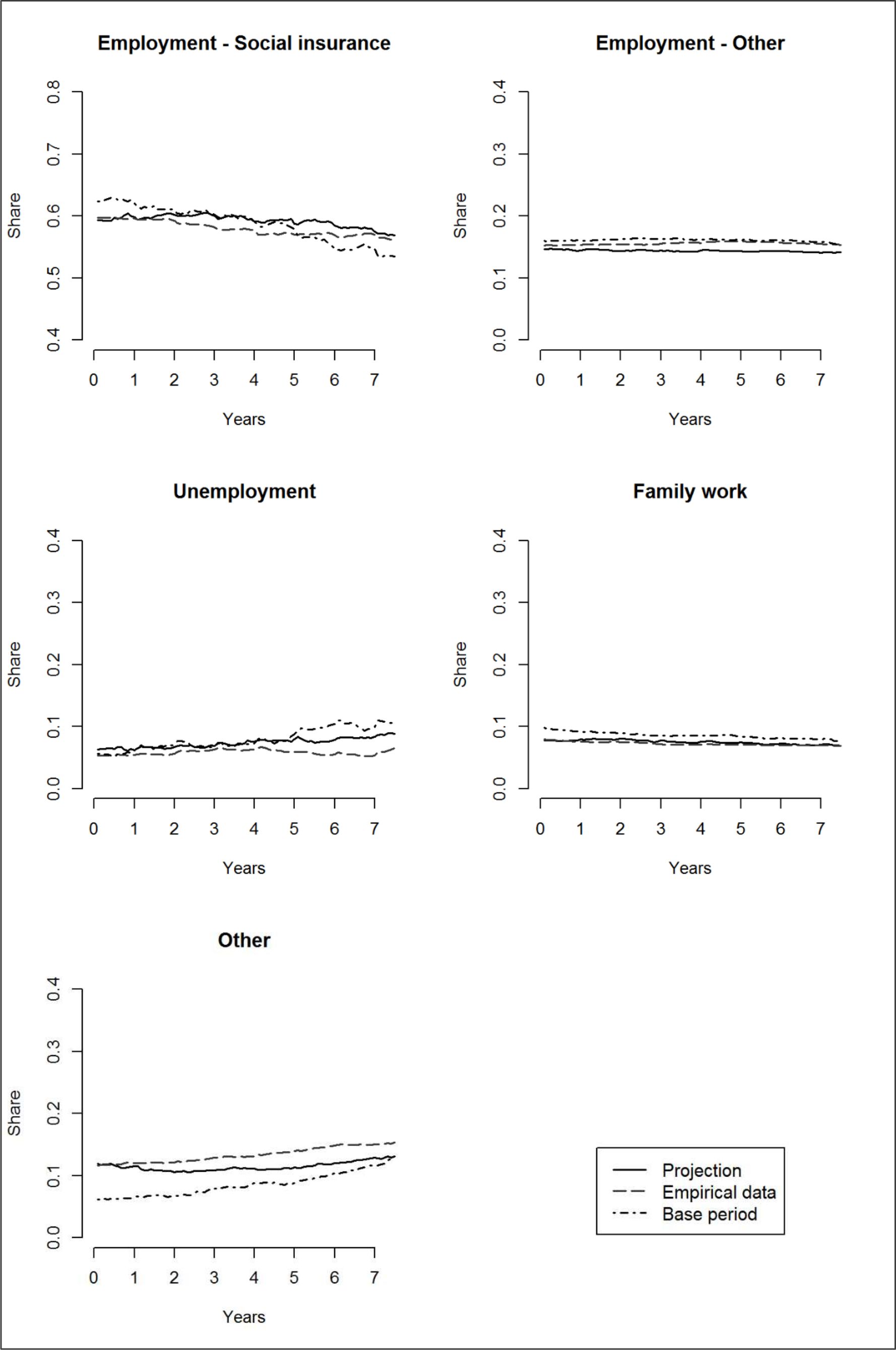
The first indicator to consider on the aggregate level is the share of states per month and how it develops over time during the projection. As an introductory overview Figure 1 shows the shares of SES for the projected, empirical and base data without differentiation of the population.6 The horizontal axis shows the time in years even though the calculations are actually carried out on a monthly basis. Please note that the range of the vertical axis for Employment – Social insurance differs from the other graphs. Even though the differing ranges might be misleading at a first glance, focussing on the relevant segment of the axis does make it easier to see the differences.
Development of SES states, total of the population.
Source: AVID 2005 and IAV 2009, own calculations.
The first impression of the projection is very positive. The projected distribution of states mirrors the empirical distribution of states almost exactly with an average deviation of only 1 percentage point (maximum 3 percentage points). For the share of unemployment there is however an increasing difference during the observation period, amounting at the end to around 3 percentage points. This is most certainly due to the developments in the base period: Here, we observe an increasingly higher share of unemployment over the years which is even higher than the share of this SES in the projection. This phenomenon and how the model was restricted to not pick up the full extent of this development is discussed further with the groups specific results for East Germany. With SES Other there are also similar differences between projection and empirical data. Most probably this is due to the empirical increase in marginal employment, but since this is a category which comprises several different SES a substantial explanation is difficult.
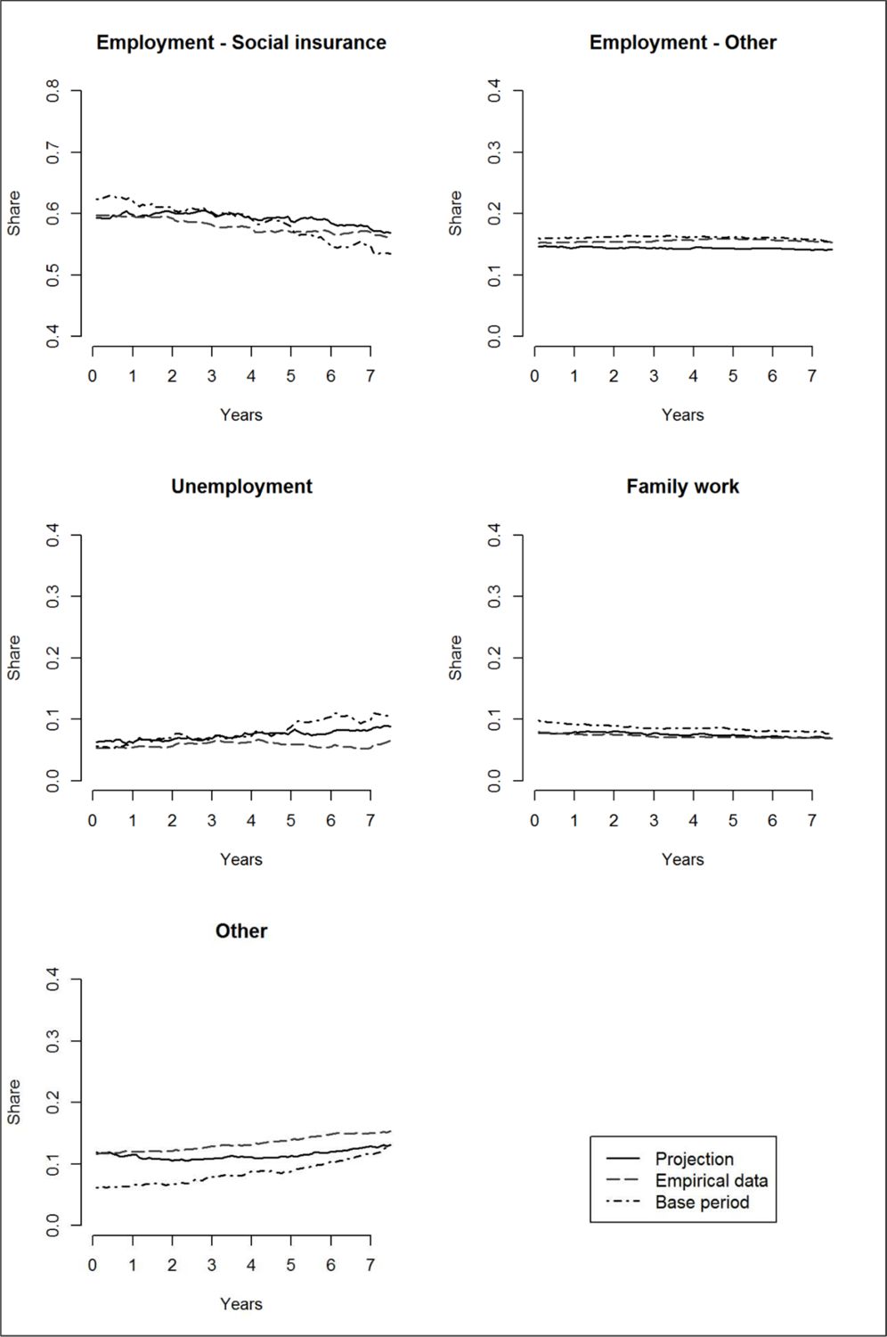
Figure 2 presents the results for West German men. For this subgroup, the picture fits even better with an average deviation of 0 percentage points. In the projected data the share of the most relevant SES Employment – Social insurance is at the maximum 2 percentage points lower than in the empirical data and correspondingly the share of unemployment is at the maximum 3 percentage points higher. Considering the development in the base period where we observe a still lower share of Employment – Social insurance these differences seem small enough and the development trend for Employment – Social insurance was actually forecast quite well. The model translates the increasing share of unemployment in the base period – quite correctly in a modelling logic – into higher aggregate levels of unemployment in the projection which then did not materialise since the situation on the labour market in Germany improved from 2005.

Development of SES states, West German men.
Source: AVID 2005 and IAV 2009, own calculations.
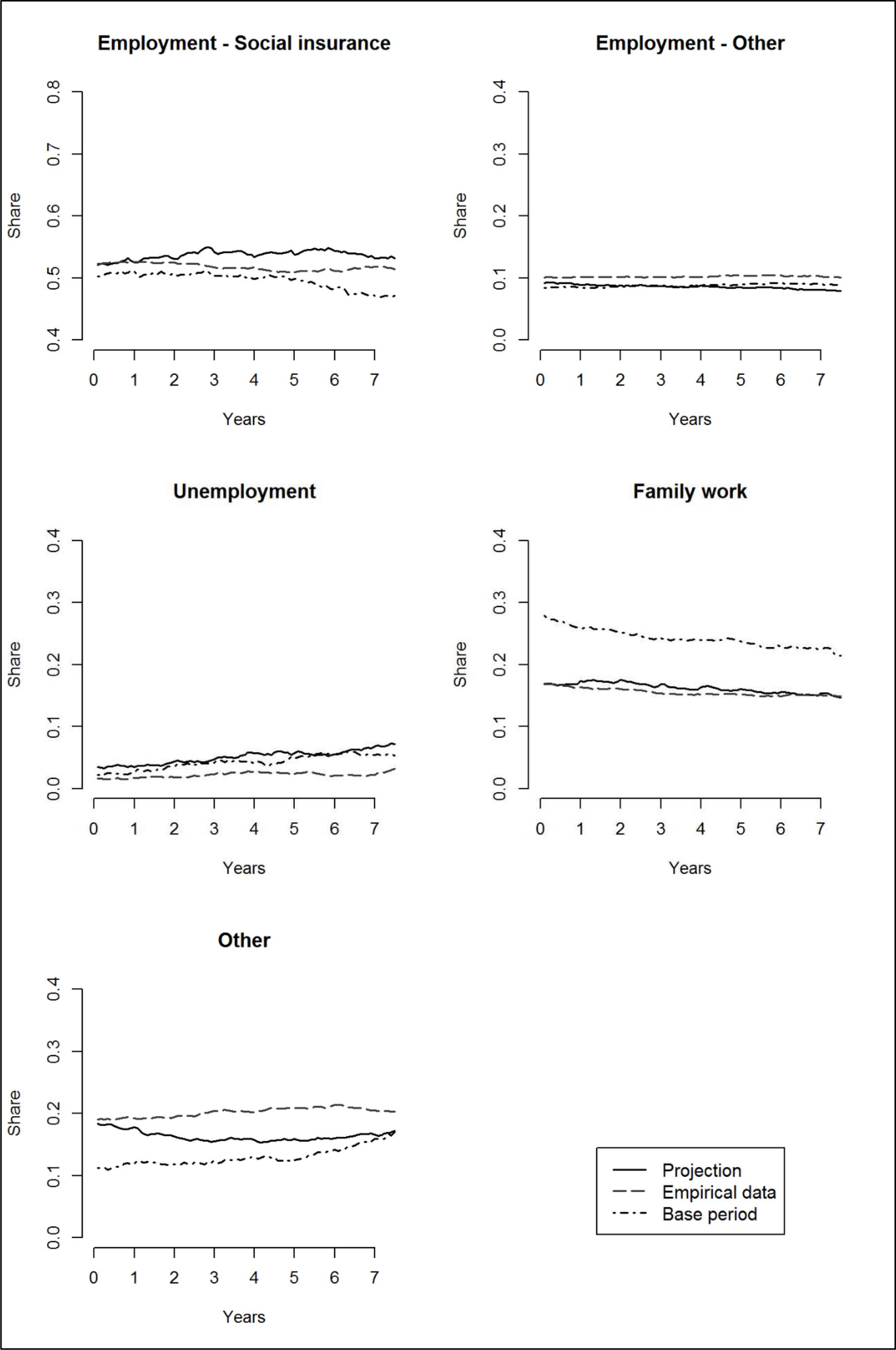
The findings for West German women are presented in Figure 3. The average deviation of the projected and empirical data is 2 percentage points, but again we find a higher share of unemployment in the projected data than was empirically observed. The maximal difference between the two data sources in this case is almost 5 percentage points. Considering that the maximum share of unemployment in the empirical data is only 3 percent this difference seems rather large. However, the projected trend seems to mirror the developments in the base period very closely, while the empirical development followed a completely different route.

Development of SES states, West German women.
Source: AVID 2005 and IAV 2009, own calculations.
More importantly though, in the projection as well as in the empirical data we see a share of Employment – Social insurance which is higher than expected considering the base period data. This trend of an increasing female labour market participation is well documented for West German women and was reproduced surprisingly well in the model (Wanger 2015).
West German women are the only subgroup with a high share of SES Other (up to 21% in the empirical data). This is mostly due to the fact that a lot of West German women are not regularly employed but prefer marginal employment. At the end of the base period we observe an increase in SES Other which the model translated into a higher share in the projection, however, the actual empirically observed levels are even up to 5 percentage points higher.
Compared to the other subgroups West German women show a higher diversity of states: The share of Employment – Social insurance is still the most dominant one, but with a share between 47% and 55% (depending on the point in time and the data source) it is low compared to the other groups. The shares of Family work (between 17% and 20%) and SES Other (between 11% and 21%) are correspondingly high. Greater heterogeneity and discontinuity of individual life courses which are well documented for West German women compared to their male counterparts translate into higher diversity on the aggregate level as well (Klammer, Bosch, Helfferich et al. 2011).
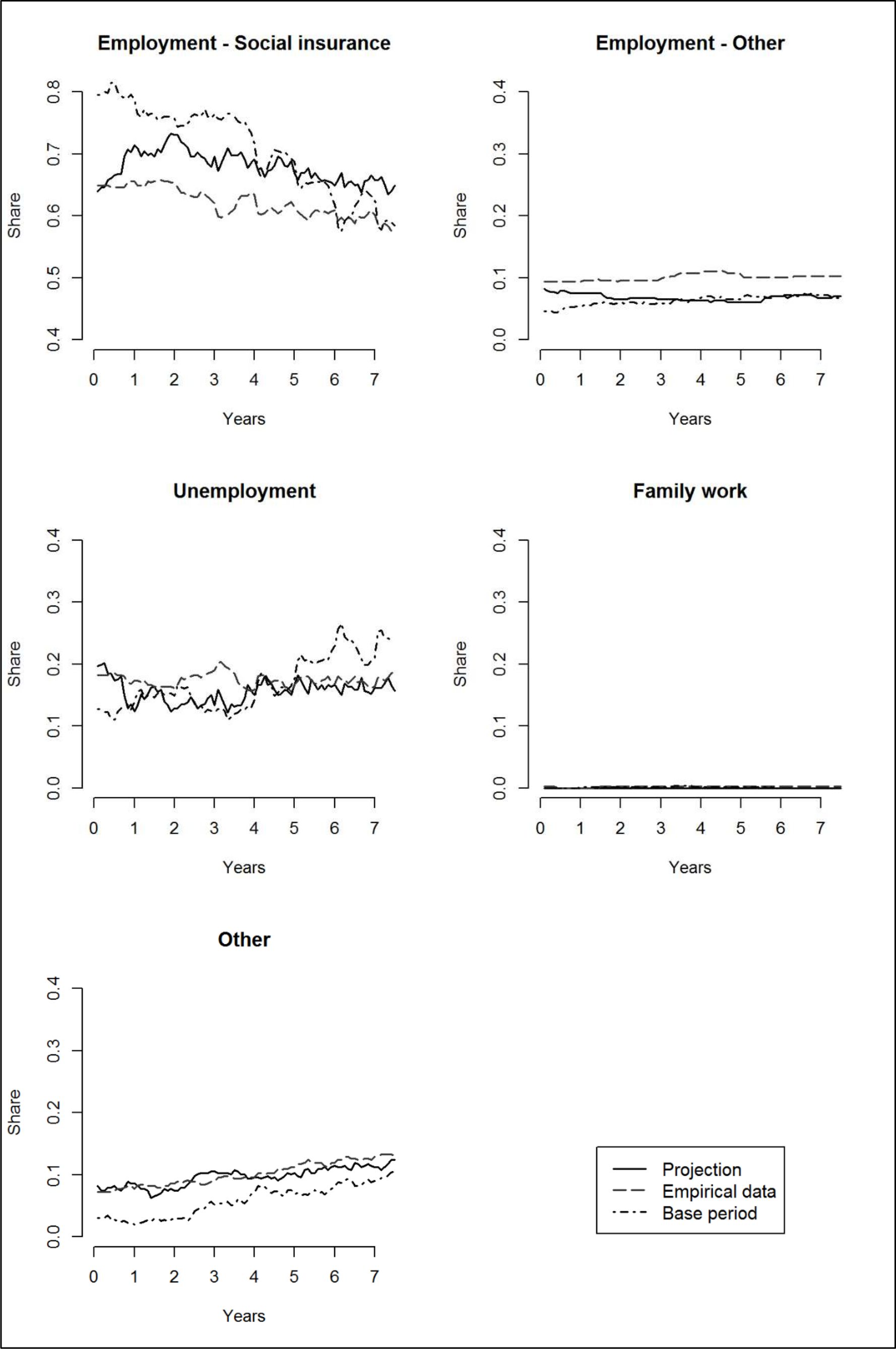
Period effects present particular challenges for the alignment of microsimulation models. Due to the turbulent transition period in the 1990ies, the projection of East German life courses turned out to be much more complex than the projection of West German ones. During the base period the share of Employment – Social insurance for East German men dropped from over 80% to less than 60% and at the same time the level of unemployment more than doubled from 12% to 25% (Figure 4). This challenge is reflected in the projection results: While the average overall deviation is still only 2 percentage points, the share of Employment – Social insurance is at the maximum 11 percentage points higher in the projection than in the empirical data while the shares of SES Unemployment and Employment – Other are too low (maximally 7 and 5 percentage points) compared to the empirical data.

Development of SES states, East German men.
Source: AVID 2005 and IAV 2009, own calculations.
The increasing share of unemployment observed in the base period was to some extent corrected for in the modelling process so that the amount of unemployment would not build up to an implausible degree in the projection period. For this purpose biographical SES ratios were calculated and the transition probabilities were adjusted so that the ratio for Unemployment in the projection period stayed roughly the same as in the base period (Schatz 2010: 54f).7 This intervention certainly accounts for the surprising stability of SES Employment – Social Insurance and Unemployment in the projection data. But while the intervention seems to have regulated the amount of unemployment towards the end of the observation period quite well, it is most certainly also responsible for the – in hindsight too high – projected level of Employment – Social insurance.
Figure 5 shows the results for East German women. The projected and empirical distributions fit remarkably well (average deviation 1 percentage point and maximal deviation 4 percentage points), especially considering the pronounced negative trend in the base period for Employment – Social insurance. As for East German men the transition probabilities were corrected for to avoid further implausible increases of the level of unemployment. The high share of unemployment in the base period thus did not carry over into the projection.

Development of SES states, East German women.
Source: AVID 2005 and IAV 2009, own calculations.
Contrary to East German men we do not find the increasing effect of the intervention on the levels of Employment – Social insurance though. This certainly reflects that the drop in Employment – Social insurance in the base period was not quite as sharp for East German women as it was for East German men, so there was less to correct for. Another interfering factor might also be the development of marginal employment, which in East Germany provides an alternative to being unemployed. The increase in SES Other for East German women during the base period is mostly due to an increase in marginal employment. This increasing trend in the base period results in a stable and comparably high share of SES Other in the projection which fits well with the empirical data.
To complete the picture on the aggregate level, Figure 6 presents the corresponding transversal entropies for all subgroups and comparison periods. For the total of the population as well as for West German men and women, the development of the transversal entropy measure seems unremarkable. There are no major deviations or discrepancies.
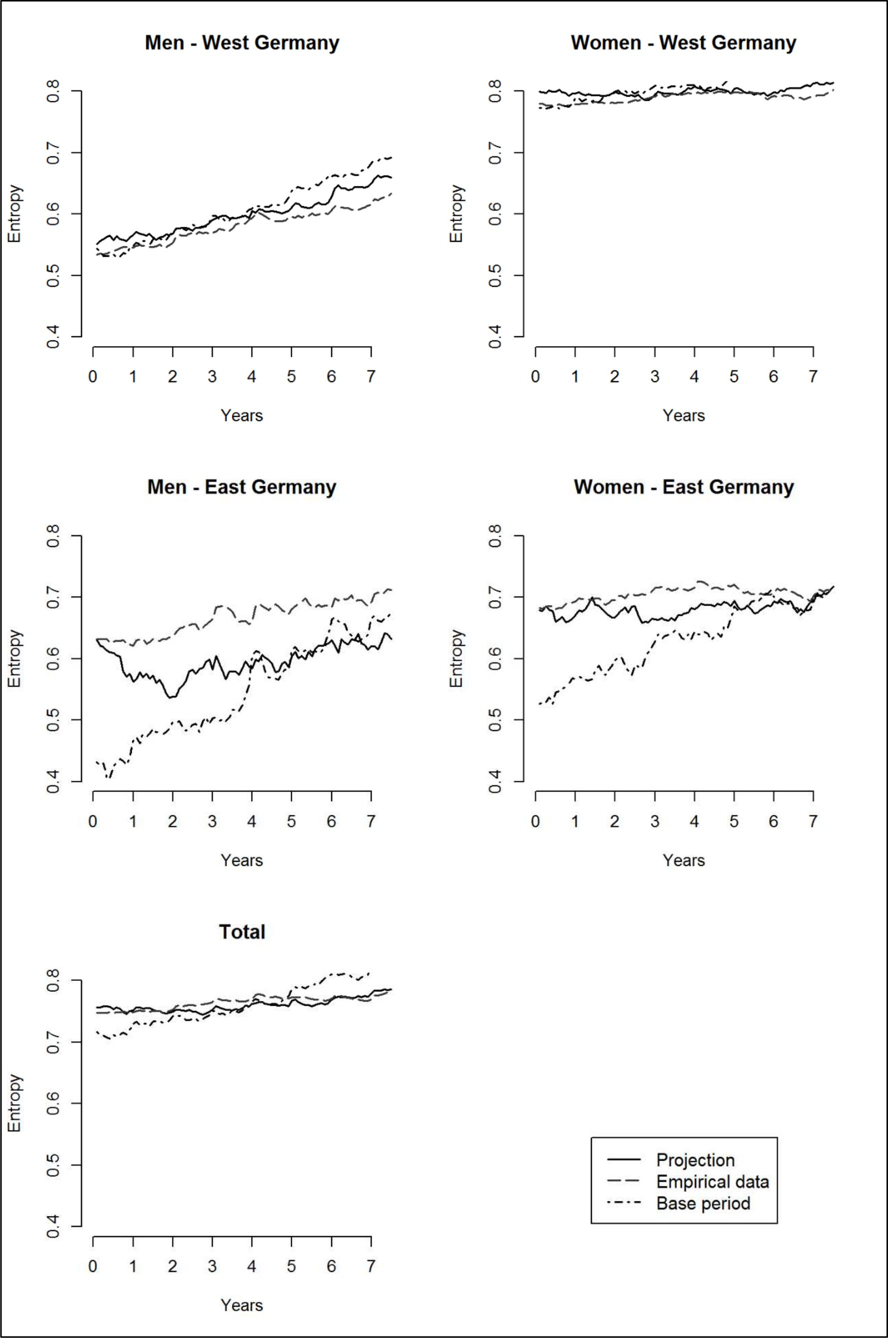
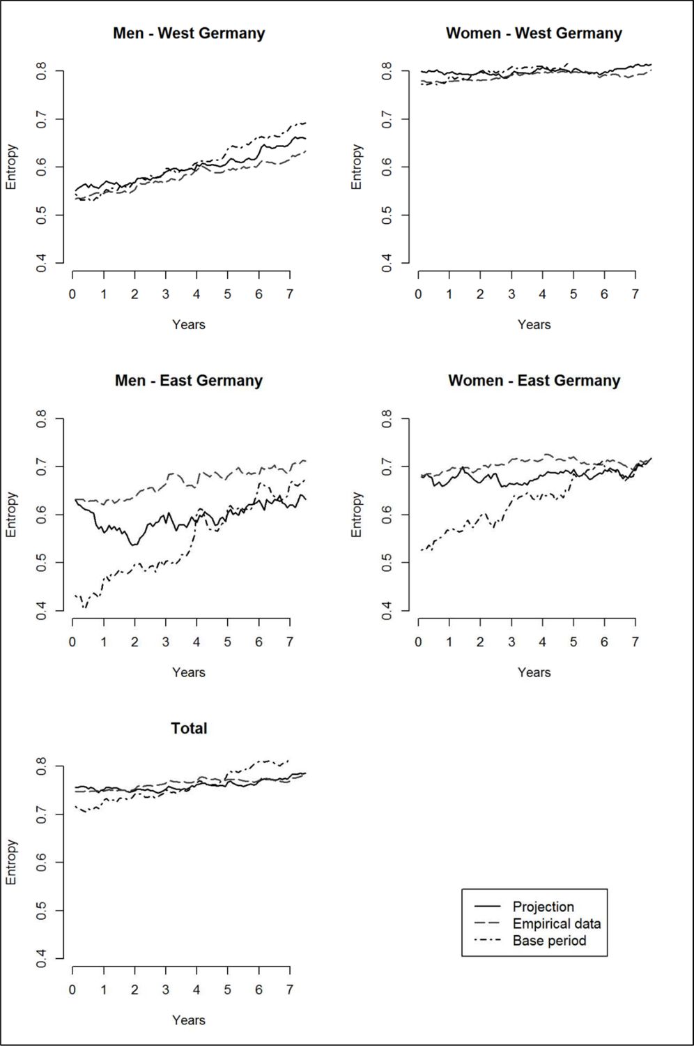
Transversal entropies.
Source: AVID 2005 and IAV 2009, own calculations.
Generally, in the base period there is a pronounced increase in entropy which reflects the situation on the labour market in Germany in the 1990ies and early 2000s. The decrease in Employment – Social Insurance and the increase in Unemployment, and to a lesser extent in self-employment and marginal employment which were discussed above result in a greater diversity of states at each point in time and in higher transversal entropies.
For West German men we observe a slightly increasing trend in all three datasets, corresponding to the decreasing trend in Employment – Social insurance (Figure 2) and indicating a higher diversity of states towards the end of the observation periods. The trend is most pronounced in the base period data and least obvious in the empirical data.
West German women show the highest entropy level of all subgroups (around 0.8). This is not surprising as for West German women we observe a higher diversity of states compared to the other groups (Figure 3) which manifests in continuously high levels of transversal entropy.
For East Germany the transversal entropies are all in all less homogenous than the ones for the West German subgroups. For East German men we observe a steep increase during the base period, an oscillating pattern for the projection and a more or less level but comparably high line for the empirical data. This is an indication of the difficulties encountered in the projection which are created by the choice of base period. East German men start with the lowest entropy levels, a legacy of the labour market situation in the GDR: Of all the subgroups they are the ones with the lowest diversity of states and the highest level of Employment – Social insurance. During the base period there is a strong increase in entropy, corresponding to the fast changes in the economic landscape and the rising levels of unemployment. As discussed before, the projection should not carry this development further without any correction, and the model was adapted to take less of the historical information on board, which in turn produces a more erratic behaviour during the projection.
The development of the transversal entropies for East German women is similar but less extreme. The entropies referring to the base period increase over the observation period while the ones for the projection and empirical data are more or less stable on an overall higher level. At the end of the observation periods we observe just about the same entropy values. For East German women the increase of the entropy values in the base period was less pronounced than for East German men, partly because they start from a higher level. The corrections during the projection were thus less intervening than the ones for East German men.
3.2 Individual level
This section focuses on the individual level and the longitudinal characterization of the sequences. The first indicator in this section refers to the content dimension or the average extent to which different SES are present in the individual life courses. Table 4 shows the mean cumulative durations and the related standard deviations (SD) for each SES in months.
Cumulative duration of states (in months).
| Projection | Empirical data | Base period | |||||
|---|---|---|---|---|---|---|---|
| Mean | SD | Mean | SD | Mean | SD | ||
| Men West | Employment – Social insurance | 56.8 | 40.0 | 57.4 | 41.3 | 55.1 | 40.9 |
| Employment – Other | 23.4 | 37.8 | 23.6 | 38.7 | 25.2 | 39.3 | |
| Unemployment | 4.3 | 14.1 | 3.1 | 13.2 | 4.2 | 13.6 | |
| Family work | 0.2 | 4.2 | 0.1 | 2.4 | 0.2 | 3.6 | |
| Other states | 5.2 | 17.0 | 5.7 | 19.8 | 5.3 | 17.0 | |
| Women West | Employment – Social insurance | 48.3 | 38.1 | 46.6 | 42.6 | 44.7 | 41.2 |
| Employment – Other | 7.7 | 23.9 | 9.2 | 26.4 | 7.9 | 24.6 | |
| Unemployment | 4.6 | 12.7 | 2.0 | 9.3 | 3.9 | 12.7 | |
| Family work | 14.6 | 27.9 | 14.0 | 30.8 | 21.8 | 35.9 | |
| Other states | 14.7 | 26.6 | 18.2 | 33.3 | 11.7 | 25.9 | |
| Men East | Employment – Social insurance | 61.1 | 35.5 | 55.9 | 39.3 | 63.7 | 29.5 |
| Employment – Other | 6.1 | 20.8 | 9.1 | 25.7 | 5.7 | 19.5 | |
| Unemployment | 14.0 | 22.2 | 15.8 | 29.2 | 15.3 | 21.1 | |
| Family work | 0.0 | 0.0 | 0.2 | 3.5 | 0.1 | 1.8 | |
| Other states | 8.7 | 19.9 | 9.1 | 24.0 | 5.2 | 15.0 | |
| Women East | Employment – Social insurance | 55.8 | 32.6 | 54.5 | 39.6 | 57.4 | 31.9 |
| Employment – Other | 4.8 | 17.6 | 5.6 | 20.8 | 3.0 | 13.3 | |
| Unemployment | 17.1 | 24.6 | 17.6 | 30.7 | 20.4 | 25.1 | |
| Family work | 1.8 | 9.0 | 2.4 | 13.4 | 1.8 | 11.2 | |
| Other states | 10.6 | 21.7 | 10.0 | 24.4 | 7.3 | 19.7 | |
-
Source: AVID 2005 and IAV 2009, own calculations.
For West German men, there are virtually no differences between the projection and the empirical data (Table 4). But they are also the least interesting of the subgroups from a methodological point of view: The model should produce good results with stable, clear-cut employment histories which are typical for West German men.
West German women also show a good resemblance between the simulated and the empirical data, although they usually have more discontinuous employment histories than their male counterparts. Apart from that, they are a good example of how dynamic microsimulation models are not mere transfer modules which reproduce patterns of the past. Instead, the different types of covariates are making use of the past for informed guesses on the future and capture important trends. For example, while women in the base period accumulate almost 22 months of family work, the younger cohorts in the projection only accumulate around 15 months, which is much closer to the actual empirical value of 14 months.
The projected cumulative values for East German men and women also fit quite well with the empirically observed ones. For the men the average amount of SES Employment – Social insurance might be comparably high (61 months in the projection vs. 56 months in the empirical data) while the average amount of Employment – Other seems low (6 months projected vs. 9 months empirically), but the overall picture is very positive, especially considering the developments in the base period discussed above.
One aspect concerning SES Unemployment seems especially noteworthy: For East German men and women we find high standard deviations in the empirical data compared to the other data sources. This variability is a new development in East Germany and could thus not be anticipated by the model.
In the following we will consider the structure of the sequences and look at findings for the complexity index (Table 5). For all groups the mean complexity indices calculated on the basis of the empirical data are lower than the ones we find for the projection or for the base period data. This is especially true for East German men and women. Here it becomes apparent again that the base period covered a special situation in Germany which did not continue along the same lines afterwards. East German men seem to be an especially difficult case again: The standard deviation in the projection data is very high compared to the other data points and to the other subgroups. There is no obvious explanation for this fact but maybe the altered transition probabilities which were introduced into the model to deal with the SES “Unemployment” lead to this implausibly high amount of variance.
Complexity index.
| Projection | Empirical data | Base period | ||
|---|---|---|---|---|
| Men West | Mean | 0.02 | 0.01 | 0.03 |
| SD | 0.04 | 0.03 | 0.05 | |
| Maximum | 0.27 | 0.26 | 0.35 | |
| % Minimum 0 | 66.6 | 84.3 | 70.7 | |
| Women West | Mean | 0.05 | 0.02 | 0.03 |
| SD | 0.05 | 0.04 | 0.06 | |
| Maximum | 0.27 | 0.26 | 0.37 | |
| % Minimum 0 | 43.2 | 77.5 | 62.3 | |
| Men East | Mean | 0.09 | 0.03 | 0.08 |
| SD | 0.12 | 0.06 | 0.08 | |
| Maximum | 0.46 | 0.25 | 0.32 | |
| % Minimum 0 | 51.3 | 67.4 | 33.8 | |
| Women East | Mean | 0.07 | 0.03 | 0.08 |
| SD | 0.07 | 0.05 | 0.08 | |
| Maximum | 0.30 | 0.24 | 0.30 | |
| % Minimum 0 | 29.7 | 66.3 | 33.6 |
-
Source: AVID 2005 and IAV 2009, own calculations.
The same impression is conveyed when we look at the maximal complexity values in the projected data (Table 5). The maximal value for East German men seems implausibly high compared to the other values.8 And there seems to be a clear East West difference. For West German men and women the projected and empirical maximal values are virtually the same while the maximal value in the base period is much higher. For East Germans the base period and projected data show high maximal values, while the empirical maximal values are lower. We thus observe a convergence in the empirical data where the maximal values are almost exactly the same over all the subgroups.
Lastly, we take a look at the share of respondents with a complexity index of 0 (Table 5). This indicates that they spend the whole observation time of 90 months in one single state. For all groups we find the highest share of respondents with complexity 0 in the empirical data. For West German men the share is 84%. This means that more than 4 out of 5 of them have not experienced a single transition. The share is lower for West German women with around 3 out of 4 (76%) and still lower for East German men and women with around 2 out of 3 (67% and 66%). Overall we find a remarkable stability of the empirical employment histories though.
The projection does not capture this empirically observed stability very well. On the contrary, for most subgroups the share of respondents with a complexity index of 0 is even lower in the projection than in the base period. This is especially true for West German women where the difference amounts to almost 20 percentage points. The odd ones out are again East German men. For them, the share of respondents with a complexity index of 0 is much higher in the projection data than in the base period data (17 percentage points). There seems to be no ready explanation for this finding, especially considering that in this subgroup we also find a high mean complexity and an extremely high maximum value for the complexity index.
To complete the picture Table 6 shows the share of respondents whose employment histories did not contain a certain SES at all (0 months), only contained one certain SES (90 months), or who find themselves in between these extreme values (1–89 months).9 A pattern is immediately obvious: The shares in the simulation data for the two extreme points 0 months and 90 months are notably lower than the ones in the empirical data.10 This is another general indication for the fact that the projection might not produce entirely satisfying results on the individual level when not averages but the underlying distribution of SES episodes is concerned.
Distribution of cumulative duration of states (in %).
| Months | Projection | Empirical data | Base period | |||||||
|---|---|---|---|---|---|---|---|---|---|---|
| 0 | 1–89 | 90 | 0 | 1–89 | 90 | 0 | 1–89 | 90 | ||
| Men West | Employment – Social insurance | 26.6 | 30.2 | 43.2 | 31.4 | 13.0 | 55.6 | 31.1 | 24.9 | 44.0 |
| Employment – Other | 69.6 | 9.7 | 20.7 | 71.0 | 5.3 | 23.7 | 68.8 | 7.1 | 24.1 | |
| Unemployment | 82.3 | 17.4 | (0.3) | 90.2 | 8.7 | 1.1 | 83.6 | 15.9 | 0.5 | |
| Family work | 99.4 | (0.4) | (0.2) | 99.6 | (0.4) | - | 99.7 | (0.2) | (0.1) | |
| Other states | 79.0 | 18.8 | 2.2 | 88.5 | 7.5 | 4.0 | 78.3 | 19.5 | 2.2 | |
| Women West | Employment – Social insurance | 27.4 | 47.4 | 25.2 | 41.1 | 16.2 | 42.8 | 39.1 | 29.0 | 31.9 |
| Employment – Other | 88.9 | 4.8 | 6.3 | 88.0 | 3.4 | 8.6 | 89.7 | 3.3 | 7.0 | |
| Unemployment | 76.6 | 23.2 | (0.2) | 91.6 | 8.0 | (0.4) | 84.4 | 15.3 | (0.3) | |
| Family work | 66.7 | 27.2 | 6.1 | 79.6 | 8.2 | 12.2 | 66.8 | 16.4 | 16.8 | |
| Other states | 61.3 | 33.3 | 5.4 | 71.3 | 15.2 | 13.5 | 69.6 | 24.2 | 6.2 | |
| Men East | Employment – Social insurance | 8.9 | 47.1 | 44.0 | 25.8 | 29.3 | 45.0 | 5.4 | 65.0 | 29.6 |
| Employment – Other | 88.5 | 7.0 | 4.4 | 87.4 | 4.4 | 8.2 | 88.8 | 7.9 | 3.3 | |
| Unemployment | 55.5 | 44.5 | - | 64.9 | 26.5 | 8.7 | 43.0 | 57.0 | - | |
| Family work | 100.0 | - | - | 99.5 | (0.5) | - | 99.7 | (0.3) | - | |
| Other states | 67.0 | 30.2 | 2.8 | 80.6 | 13.8 | 5.6 | 67.7 | 31.2 | (1.1) | |
| Women East | Employment – Social insurance | 9.5 | 68.6 | 21.9 | 26.5 | 28.6 | 45.0 | 8.4 | 63.4 | 28.1 |
| Employment – Other | 88.8 | 8.4 | 2.9 | 91.8 | 3.0 | 5.1 | 92.7 | 6.6 | (0.8) | |
| Unemployment | 47.0 | 51.8 | (1.1) | 65.0 | 26.1 | 9.0 | 40.7 | 58.2 | (1.1) | |
| Family work | 93.9 | 5.9 | (0.2) | 96.2 | 2.3 | (1.5) | 95.7 | 3.4 | (0.9) | |
| Other states | 53.1 | 43.2 | 3.6 | 77.7 | 16.6 | 5.7 | 69.0 | 28.3 | 2.6 | |
-
Source: AVID 2005 and IAV 2009, own calculations, ( ) n < 10, – n = 0.
This fact is relevant as it seems that there was a general trend towards more inequality after 2001. For example, the empirical data show a higher share of respondents who were not affected by unemployment than the projection. This can partly be attributed to a better situation on the labour market, but it is also an indicator for more inequality as less people show longer periods of unemployment.
The following paragraphs look more closely at the results for the different subgroups (Table 6). For West German men there are only small differences. As noted before, for projection purposes they are the easiest of the various subgroups. For West German women there are two points which stand out: First of all, in the projection both shares for the extreme values of SES Employment – Social insurance are very low. Together they cover just over half of the female West German respondents (53%) while in the empirical data they cover more than four out of five (84%). This cannot be attributed to the base period data since here the two extreme values together cover a share of 71%.
Secondly, the extreme values for SES Family work are notable. The share of West German women with no Family work is about 13 percentage points lower in the projection than in the empirical data. But the projected share is close to the share in the base period. The share with the maximum value of 90 months is also much lower in the projection than in the empirical data, but both shares are lower than the one in the base period data. It seems that the projection has captured that there has been some sort of change in the family care behaviour of West German women, but it has not been able to line out the details of these changes quite correctly.
For East German men we look at the two pivotal SES Employment – Social insurance and Unemployment. The share of East German men with zero months in Employment – Social insurance is below a tenth (9%) in the projection – probably because of an even lower share in the base period (5%) – while it is over a forth (26%) in the empirical data. The share of men with a maximum of 90 months is virtually the same in the projection and empirical data (44% and 45%); even though it is around 15 percentage points lower in the base period (30%).
As far as SES Unemployment is concerned, the highest share of men without the SES can be found in the empirical data (65 %), the lowest share can be found in the base period (43 %) and the projected share is almost exactly in the middle between these two values (56 %). The maximum of 90 months cannot be observed in the base period or in the projection, but in the empirical data there is a surprisingly large share of 9% of East German men who spent the entire observation period in unemployment.
This pattern of an increasingly divided labour force is equally apparent with East German women. The share of women with zero months of Employment – Social insurance is around ten percent in the projection (10%) and the base period (8%) but 27% in the empirical data. The share of women who reach the maximal value is 22% in the projection, 28% in the base period and 45% in the empirical data. As far as Unemployment is concerned, in the projection almost half of the East German women (47%) show the minimum value of zero, while this share is as high as two thirds (65%) in the empirical data and the lowest with 41% the base period data. The maximum value is not reached by a statistically sufficient number of women in either the projection or the base period, in the empirical data though, we find almost a tenth (9%) of women with 90 months of continuous unemployment.
4. Discussion
The findings presented in this paper highlight different aspects of the simulation. Overall, the results are encouraging. The projected average values, which are most commonly considered when validating a model, fit very well with the empirical data. The deviation between the projected and empirical shares is only 1 percentage point on average. If we consider the structure of the employment histories though, we find bigger differences. The projection spread the SES over too many individuals and thus underestimated the stability of employment histories and the amount of inequality. This phenomenon is apparent in all the subgroups considered, but it is especially pronounced for East German men and women whose life courses are more challenging to project due to a strong period effect.
Since the model set-up is explicitly longitudinal we would expect discontinuity and spell lengths to be adequately accounted for. The major source for the observed discrepancy between the projected and empirical data is therefore the situation in the base period. The findings show that we can at least partly attribute the surplus of discontinuity to the period effect and the amount of discontinuity present in the base period. The stability observed in the empirical data is an expression of social change which could not be foreseen by the model.
In case of the AVID the modifications of the transition probabilities for East Germany might also have led to shorter spell lengths and higher discontinuity measures. However, with the retrospective comparisons presented here it is not possible to quantify to which extent this might be the case.
The retrospective validation of the AVID model also allows for another interesting observation. We can get a feeling for the importance of the specification of the base period by comparing the results for East and West Germany. While the 1990ies were turbulent times for the whole of Germany, the East of the country underwent a complete transition. At the end of the decade just about everything had changed: the political system, the economic system, the labour market, and the educational requirements for successful participation in the labour market. This means that East Germans had very continuous employment histories as a legacy of the state-directed economy which were interrupted quite suddenly for a big part of the population. As expected, the comparisons presented above show clearly that the projection was much closer to the empirical data for West Germany than for East Germany and we observe the highest deviation between projection and empirical data for East German men for whom the changes were most pronounced. However, considering the vast and sudden changes, the projection for East Germany was not very far off the empirical mark either. As far as the validation process is concerned, the AVID model seems to be quite robust which suggests that while the choice of base period does matter it is only one part of the model set-up.
For microsimulation modelling this is an encouraging result. With the last financial crisis and the repercussions for national economies and labour markets, more models will have to deal with turbulent base periods and parameters which are influenced by period effects and external shocks. And while the findings presented in this paper suggest that the projections can still be quite accurate, they also highlight the need for validation and more precisely for retrospective validation which goes further than average values.
5. Conclusion
This paper was concerned with a retrospective comparison of projected and empirical data on life courses. The overall aim of the paper was to develop indicators which help to decide questions on how good a simulation model is and whether we can use the results without reservations. The proposed indicators cover different aspects of the simulation such as the aggregate and individual level, the different dimensions of content and structure and use averages as well as extreme values to get a deeper understanding of the results.
In case of the AVID model the answer to the above questions is yes and no. Overall there is a good resemblance between the projection and the empirical data and no deteriorating trend could be detected towards the end of the observation period. This is important since an increasing difference between the projection and the empirical data would suggest that the results at the end of the projection period, which is considerably longer than the observation period in this paper, could be very far off the empirical benchmark.
The average values on the aggregate and the individual level were very similar in the projection and the empirical data, but the projection underestimated the stability of the employment histories. This can be explained by the developments in the base period, but it is nevertheless an important information for the application and interpretation of the results. A higher stability of employment histories in the context of similar average values means higher inequality as i.e. the same amount of unemployment is concentrated on fewer people who face longer episodes of unemployment or even continuous unemployment.
Usually in the development of a microsimulation model resources for in depth validation are limited. But the results presented in this paper suggest that it is worthwhile taking a detailed look and it might even be helpful to calculate these indicators for different stages of the model development and find out when differences occur and if they increase or decline in the development process.
Footnotes
1.
During the development of the AVID model other and broader validation activities were carried out routinely which are not commented on here. For example the model was run for the base period to check if the development of the SES was reproduced correctly (Schatz 2010).
2.
Harding, Keegan and Kelly (2010) set up their validation along similar lines even though they do not discuss the levels and dimensions explicitly.
3.
The maximum value of the entropy given the size of the alphabet a is defined as hmax = log a.
4.
Unweighted results are presented throughout the paper. Weighting only leads to minimal differences.
5.
An earlier version of this analysis with a limited number of birth cohorts can be found in Frommert (2014).
6.
Please refer to Table 3 for the number of respondents.
7.
Further adjustments were necessary for marginal employment and invalidity (Schatz 2010: 54f).
8.
The maximal value is not an extreme outlier as could be assumed at first sight.
9.
The shares for the maximum of 90 months for the different SES add up to the share of respondents with a complexity index of 0. Any discrepancies are due to rounding error.
10.
The same pattern occurs with a tolerance margin of three months.
References
-
1
What are the driving forces behind trends in inequality among pensioners? Validating MIDAS Belgium using a stylized modelIn: G Dekkers, M Keegan, C O’Donoghue, editors. New pathways in microsimulation. Farnham: Ashgate Publishing Limited. pp. 287–304.
-
2
After the fall of the wall: Life courses in the transformation of East GermanyStanford, California: Stanford University Press.
-
3
Gut geschätzt oder weit daneben? Ein Vergleich simulierter und empirischer Erwerbsverläufe auf Basis der Erhebungen “Altersvorsorge in Deutschland 2005” und “Individuelle Altersvorsorge 2009”Deutsche Rentenversicherung 69:178–192.
-
4
Analyzing and visualizing state sequences in R with TraMineRJournal of Statistical Software 40:1–37.
-
5
Indice de complexité pour le tri et la comparaison de séquences catégoriellesExtraction et gestion des connaissances (EGC 2010), Revue des nouvelles technologies de l’information E-19:61–66.
-
6
Validating a dynamic population microsimulation model: Recent experience in AustraliaInternational Journal of Microsimulation 3:46–64.
-
7
Altersvorsorge in Deutschland 2005: Alterseinkommen und BiographieAltersvorsorge in Deutschland 2005: Alterseinkommen und Biographie, DRV-Schriften 75 and BMAS-Forschungsbericht 365, Berlin.
-
8
Neue Wege – Gleiche Chancen: Kurzfassung des ersten Sachverständigengutachtes zum Ersten Gleichstellungsbericht der BundesregierungIn: U Klammer, M Motz, editors. Neue Wege – Gleiche ChancenNeue Wege – Gleiche Chancen: Expertisen zum Ersten Gleichstellungsbericht der Bundesregierung. Wiesbaden: VS Verlag für Sozialwissenschaften. pp. 13–43.
-
9
Teilzeitarbeit im Lebenslauf von abhängig beschäftigten FrauenIn: U Klammer, M Motz, editors. Neue Wege – Gleiche Chancen: Expertisen zum Ersten Gleichstellungsbericht der Bundesregierung. Wiesbaden: VS Verlag für Sozialwissenschaften. pp. 253–311.
-
10
Dynamic ModelsIn: C O’Donoghue, editors. Handbook of Microsimulation Modelling. Howard House, UK: Emerald. pp. 305–343.
-
11
Validation of longitudinal models: DYNACAN practices and plans. APPSIM Working Papers No. 8National Centre for Social and Economic Modelling, University on Canberra.
-
12
Die Aktualisierung der Studie Altersvorsorge in Deutschland: Inhaltliche und methodische Neuerungen der AVID 2002Deutsche Rentenversicherung 57:612–641.
-
13
Altersvorsorge in Deutschland (AVID) 2005: Methodenbericht Teil II: Fortschreibung und AnwartschaftsberechnungMünchen: TNS Infratest Sozialforschung.
-
14
Traditionelle Erwerbs- und Arbeitszeitmuster sind nach wie vor verbreitet. IAB Kurzbericht 4/2015Traditionelle Erwerbs- und Arbeitszeitmuster sind nach wie vor verbreitet. IAB Kurzbericht 4/2015.
-
15
Übergänge und Sequenzen: Der Einfluss von Arbeitslosigkeit auf den weiteren ErwerbsverlaufIn: R Sackmann, M Wingens, editors. Strukturen des Lebenslaufs: Übergang – Sequenz – Verlauf. Weinheim/München: Juventa Verlag. pp. 163–198.
-
16
Arbeitslosigkeit und Alterssicherung: Der Einfluss früherer Arbeitslosigkeit auf die Höhe der gesetzlichen AltersrenteZeitschrift für Arbeitsmarkt Forschung 38:493–509.
Article and author information
Author details
Acknowledgements
I would like to thank Torsten Heien, Christof Schatz, the editor of this journal and an anonymous referee for their helpful comments.
Publication history
- Version of Record published: April 30, 2015 (version 1)
Copyright
© 2015, Frommert
This article is distributed under the terms of the Creative Commons Attribution License, which permits unrestricted use and redistribution provided that the original author and source are credited.