Endogenizing take-up of social assistance in a microsimulation model a case study for Germany
- Institute for Employment Research (IAB), Germany
Abstract
Microsimulation studies typically assume that all entitlements to means-tested benefits are actually claimed by eligible households, despite a large body of research that suggests that take-up rates are substantially below 100%. The assumption of full take-up tends to exaggerate the simulated increase in caseloads and fiscal costs of a social policy reform. This paper investigates the impact of non-take-up for two hypothetical scenarios, namely increasing and decreasing the base amount of social assistance in Germany by €100 per month. We find a substantial effect of considering non-take-up on the simulated change in fiscal costs and in particular on the change in caseloads, where the full take-up assumption exaggerates the latter change by a factor of about two.
1. Introduction
An important aspect of assessing the impact of social assistance policies is to consider non-take-up of the targeted population, i.e., people might not claim a welfare benefit despite being eligible to receive it. Non-take-up has been the subject of a large number of empirical studies in recent decades (see, e.g., Blundell, Fry, & Walker, 1988; Duclos, 1995; Fry & Stark, 1987; Hancock, Pudney, Barker, Hernandez, & Sutherland, 2004; Hancock, Pudney, Sutherland, Barker, & Hernandez, 2005; Kayser & Frick, 2001; Keane & Moffitt, 1998; Moffitt, 1983; Pudney, Hancock, & Sutherland, 2006; Riphahn, 2001). Recent analyses for Germany (Bruckmeier, Pauser, Walwei, & Wiemers, 2013; Bruckmeier & Wiemers, 2012) estimate rates of non-take-up for social assistance of more than 40%.
By contrast, microsimulation studies typically assume full benefit take-up, ignoring factors impeding the claim of social assistance, e.g., stigmatization, information deficits, and complex claiming schemes. This tends to overstate the efficiency of social assistance in fulfilling the needs of the eligible population. Assuming full benefit take-up also tends to exaggerate the increase in caseloads and fiscal costs when, e.g., increasing the base amount of social assistance. Households that were borderline noneligible before the increase will have a small entitlement after the increase. For these households costs of take-up will likely exceed the utility from claiming, resulting in non-take-up.
In this paper, we investigate the importance of non-take-up regarding its impact on the outcome of a policy simulation. Because policy makers are foremost interested in reliable estimates of the fiscal costs of a reform, we simulate the effect of increasing (or decreasing) the base amount of social assistance on fiscal costs and the number of households claiming the benefit when assuming i) 100 % take-up and ii) endogenous benefit take-up.
The contribution of this paper to the literature consists in combining the method of Pudney et al. (2006) for endogenizing take-up behavior in a microsimulation model with a model of benefit take-up for Germany along the lines of Bruckmeier and Wiemers (2012) and applying this methodology to a specific policy reform using a microsimulation model based on German survey data. Our simulations show that ignoring non-take-up in a policy simulation strongly exaggerates the change in fiscal costs for social assistance and, in particular, the change in the caseloads.
The remainder of the paper proceeds as follows. In the next section we briefly lay out the framework for endogenizing benefit take-up as a component of our microsimulation model. Section 3 gives a short overview of the data and the employed microsimulation model followed by the simulation results for social assistance take-up. Section 4 presents the estimated take-up equations and demonstrates the effect of considering non-take-up in an example application that consists in increasing or decreasing the base amount of social assistance. Section 5 concludes.
2. Take-up behavior in a changing policy environment
2.1 Take-up behavior
We follow the literature on welfare benefit take-up and analyze take-up behavior within a discrete choice framework (see, e.g., Blundell et al., 1988; Bruckmeier & Wiemers, 2012; Riphahn, 2001; Whelan, 2010; Wilde & Kubis, 2005). Benefit take-up will be observed if the net level of utility from claiming a benefit exceeds the utility from not claiming the benefit. Because the decision to claim a benefit hinges on unobservable factors (perceived degree and duration of being needy, informational costs, and fear of stigmatization), estimating take-up equations requires choosing observable proxy variables for the utility and costs of claiming SA.
Assuming linear forms for the utility and costs of claiming, the probability of observing take-up (P = 1) is given by
with denoting the latent take-up propensity, where the vector of proxy variables x includes the observed characteristics that determine take-up. The benefit b is determined according to the rules of the benefit system, represented by the function b = b (y, x*, τ), which depends on earned income y, other household characteristics x*, and the parameters τ describing the tax and transfer rules. Assuming a normal distribution F (.) = Φ(.) for the error term υ leads to a (pooled) probit estimator, where Φ (.) stands for the cumulative standard normal distribution.
Alternatively, we account for the potential endogeneity of the entitlement b by estimating an instrumental variable (IV) probit model, as proposed by, e.g., Whelan (2010) and Bruckmeier and Wiemers (2012). The estimation of the IV probit requires the choice of instruments on the benefit level. Following Bruckmeier and Wiemers (2012), we use the level of household income independent of the current choice of labor supply (including pension, widow’s pension, child benefits, maternity allowance and rental income) as well as the maximum level of SA excluding housing costs.1 These instruments are determinants of the computation of the level of SA and thus satisfy the requirement that the instrument be correlated with the endogenous variable. Additionally, both of these instruments are arguably not correlated with the unobserved factors determining the take-up decision.
Finally, we exploit the panel structure of our data and estimate a random effects probit model of benefit take-up. In this model, the probability of take-up for household i in period t is given by
where εit are i.i.d. Gaussian errors with mean zero and variance , independent of the random effects vi, which are i.i.d. N(0, ). The share of the total variance contributed by the panel-level variance component is given by . In the case of ρ = 0 the random effects model coincides with the pooled probit model. Thus, a likelihood-ratio test of ρ = 0 can be employed to formally test the pooled probit against the panel probit estimator.
2.2 Policy reforms and take-up behavior
Pudney et al. (2006) discuss the possibility that take-up behavior may change after policy reforms that have an impact on benefit entitlement. This in turn requires a distinction between sunk and non-sunk claim costs. At least some fraction of take-up costs will likely be sunk in nature, especially regarding the initial take-up decision.
Sunk costs of claiming can be accounted for by specifying the take-up propensities before and after a reform (denoted by superscripts “0” and “1”, respectively) as follows:
with Pt = 1 (P*t > 0), t = 0,1 and δ the share of sunk claim costs (0% for δ = 0 and 100% for δ = +∞).2 We have redefined the variables determining take-up (including the benefit) as x = x (τ) to indicate that these variables are known functions of the parameters τ characterizing the tax and transfer system. Equation (3) also illustrates that a reform (τ0 → τ1 might not only change the individual benefit amount as well as other variables determining take-up, but also the coefficients β and the disturbances υ. Thus, ex ante analyses of a reform proposal are impossible without further assumptions. We proceed with the assumption that neither the coefficients β nor the random error υ are affected by the reforms, i.e., we assume β0 = β1, υ0 = υ1, Therefore, the policy change is assumed to be completely summarized by the transition x0 (τ0) → x1 (τ1. The assumption τ0 = τ1 seems plausible, since the random errors U represent fundamental unobserved personal attitudes towards welfare dependency that are likely not affected by a policy reform. Regarding δ, we consider the two extreme cases δ = 0 and δ = +∞, i.e., we assume the share of sunk costs of take-up to be zero or one, respectively. Since we cannot estimate the share of sunk costs of take-up from the data, this approach allows as to estimate the maximum impact of sunk costs on the simulation results.
We employ the flexible stochastic simulation approach suggested by Pudney et al. (2006) to calculate the impact of a policy change when allowing for non-take-up. The approach is outlined in Appendix A.3
3. Microsimulation model and data
We use the Tax-Transfer Microsimulation Model of the Institute for Employment Research (IAB-STSM) to simulate entitlements to SA. The IAB-STSM is based on the Steuer-Transfer-Mikrosimulationsmodell (STSM) of the Centre for European Economic Research (ZEW).4 The IAB- STSM is a static microsimulation model that consists of a detailed implementation of the German tax and transfer system as well as an econometrically estimated labor supply model. The model is mainly used for the ex ante evaluation of social policy reforms directed at low-income households in Ger-many. Its validity with regard to official statistics and its robustness referring to model assumptions and data selection has been verified in several studies (Arntz et al., 2007; Blos, Feil, Rudolph, Walwei, & Wiemers, 2007; Bruckmeier & Wiemers, 2012; Wiemers & Bruckmeier, 2009). A brief overview of the model is given in Appendix B.
The IAB-STSM is based on data from the German Socio-Economic Panel (GSOEP), a representative yearly household panel study in Germany.5 We employ the GSOEP waves 2005 to 2011 with information on approximately 11,000 households and 20,000 individuals aged 17 and older in each wave. Due to the reorganization of the welfare system in Germany in 2005 (see, e.g., Bruckmeier and Wiemers (2011) for details of the reform), we exclude data from before 2005 from our analysis.
For the period 2005 to 2011, we simulate a total of 35.2 million households (5,960 observations) eligible for SA.6 Hence, on average about five million households are eligible per wave. Table 1 shows the rates of non-take-up for each wave and pooled over all waves. Approximately 42.4 percent of all eligible households do not claim their entitlements when pooling observations. For the individual waves, rates of non-take-up range from 38.6% to 48.0%. Based on the 95% confidence intervals, the pairwise differences in the rates are in general not statistically different from zero. The resulting rates of non-take-up are comparable to the results of Bruckmeier and Wiemers (2012), who find rates of non-take-up between 41% and 49% for the years 2005 to 2007.7
Rates of non-take-up of social assistance 2005–2011
| Non-take-up Rate | 95%-Confidence Interval | |
|---|---|---|
| 2005 | 48.0 | [43.6–52.5] |
| 2006 | 42.6 | [38.6–46.6] |
| 2007 | 40.8 | [36.7–44.9] |
| 2008 | 45.3 | [40.7–49.9] |
| 2009 | 38.6 | [33.8–43.4] |
| 2010 | 38.8 | [33.4–44.1] |
| 2011 | 42.8 | [37.8–47.8] |
| Pooled | 42.4 | [40.7–44.1] |
-
Weighted non -take-up rates in percent. Source: GSOEP years 2005–2011, pooled data, IAB-STSM
4. Results
4.1 Estimation results
Table 2 reports the estimation results for three specifications of the take-up equation. See Appendix C for a brief discussion of the expected effects of the proxy variables on the utility and costs of take-up. Descriptive statistics of the regressors are given in Table 6 in Appendix D. The first column gives the result for a pooled probit model, which does not correct for the potential endogeneity bias of the level of SA. The results of the instrumental variable (IV) probit estimation for the pooled data are given in in the second column.8 Finally, estimation results for the random effects probit estimation are given in the third column of Table 2.
In general, the estimated signs of the coefficients are consistent with our expectations about the impact of the proxy variables on the take-up decision, as discussed in Appendix C, and are in line with the literature (see, e.g., Bruckmeier & Wiemers, 2012; Frick & Groh-Samberg, 2007; Whelan, 2010). The main variable of interest is the effect of the calculated monthly benefit on take-up behavior. The marginal effect of the benefit in the probit model implies that an increase of 100 € per month in SA increases the probability of take-up by 7.2 percentage points. The RE probit model gives a slightly higher effect (7.5 percentage points). Taking account of the potential endogeneity of the calculated SA using the IV probit approach reduces the marginal effect only slightly (0.9 percentage points relative to the simple probit model and 1.2 percentage points relative to the RE probit model).9 Thus, considering endogeneity of the simulated benefit only has a small impact on the marginal effects.
Marginal effects on probability of take-up (dependent variable).
| Model 1 Probit | Model 2 IV Probit | Model 3 RE Probit | |
|---|---|---|---|
| Simulated monthly benefit (in 100 EUR) | .0718*** | .0627*** | .0745*** |
| (.0016) | (.0062) | (.0023) | |
| Single | .0463*** | .0444*** | .0278 |
| (.0144) | (.0150) | (.0244) | |
| Single parent | .0529** | .0780*** | .0506 |
| (.0217) | (.0277) | (.0358) | |
| Family with children | .0112 | .0353 | .0123 |
| (.0242) | (.0299) | (.0371) | |
| Number of children aged < = 3 years | .0545*** | .0699** | .0696** |
| (.0205) | (.0230) | (.0289) | |
| Number of children age > 14 years | −.0410*** | −.0345** | −.0360* |
| (.0124) | (.0138) | (.0184) | |
| HHH retired | −.0161 | −.0528* | .0063 |
| (.0195) | (.0306) | (.0315) | |
| Disability of HHH | .0579 | .0588 | .1059** |
| (.0385) | (.0402) | (.0522) | |
| High qualif. HHH (ref.: med. qual.) | −.1322*** | −.1375*** | −.1824*** |
| (.0158) | (.0168) | (.0271) | |
| Low qualif. HHH (ref.: med. qual.) | .0302** | .0420*** | .0568*** |
| (.0128) | (.0151) | (.0216) | |
| Age of HHH | .0045*** | .0053*** | .0042*** |
| (.0004) | (.0007) | (.0007) | |
| Male HHH | .0233** | .0310** | .0371** |
| (.0110) | (.0124) | (.0187) | |
| Home owner household | −.1715*** | −.1961*** | −.2275*** |
| (.0166) | (.0224) | (.0280) | |
| Rural area (ref.: interm. area) | .0369** | .0367** | .0437 |
| (.0155) | (.0162) | (.0272) | |
| Metrop. area (ref.: interm. area) | −.0016 | −.0002 | −.0039 |
| (.0111) | (.0116) | (.0186) | |
| Eastern Germany | .1375*** | .1447*** | .1816*** |
| (.0115) | (.0126) | (.0200) | |
| EU migrants | −.0946*** | −.1035*** | −.0594 |
| (.0347) | (.0374) | (.0626) | |
| Non-EU migrants | .0111 | .0199 | .0323 |
| (.0215) | (.0231) | (.0365) | |
| Migrants with German citizenship | .0114 | .0156 | .0213 |
| (.0137) | (.0147) | (.0223) | |
| Observations | 5960 | 5960 | 5960 |
| Wald test of exogeneity: 㱲2(1) | 2.88* | ||
| (Pseudo)log-likelihood | −2749.99 | −17327.596 | −2369.8414 |
| ρ | .717 |
-
Source: GSOEP 2005–2011, own calculations. HHH stands for head of household. Wave-dummies included in all models. Standard errors in parentheses.
-
*
p < 0.1.
-
**
p < 0.05.
-
***
p < 0.01.
From the set of dummy variables on family status, the dummies for being single and being a single parent have the expected signs and are highly significant for both the probit and IV probit specifi-cations, but not for the RE probit. The number of young (old) children in the household has a significant and positive (negative) impact on the probability of take-up for all specifications. We find that having a high (low) qualification significantly reduces (increases) the probability of take-up, with a high marginal effect (in absolute value) for being highly qualified. Contrary to our expectations, we find a significant, but small positive effect of being a male head of household. The dummy for home ownership shows a very strong negative effect on the probability of claiming SA. From the set of regional dummies, the dummy for residing in eastern Germany is significant for all specifications, with a very high positive marginal effect on the take-up probability, which probably reflects a worse labor market situation than in western Germany. Finally, the dummies on migration status are in general insignificant, with the exception of the dummy which indicates being a migrant from an EU state, which has a negative impact on the take-up probability for the pooled probit and IV probit, but not for the RE probit.
Summing up, the regression results suggest that the degree of needs, measured as the SA benefit level households are entitled to, being single or being a single parent, as well as the expected duration of being needy, expressed in proxy variables like having young children, qualification, living in eastern Germany, or age, are important determinants of the take-up decision. Proxy variables that mainly measure stigmatization and information costs only seem to play a minor role in the take-up decision.
4.2 Impact of non-take-up on simulation results
We now investigate the effect of non-take-up of SA under the two hypothetical scenarios, a) increasing and b) decreasing the base amount of SA10, which is €399 per month in 2015, by €100 per month11, while all other settings of the tax and transfer system remain constant. The base scenario is given by the actual tax and transfer system in 2015, as represented in our microsimulation model. Because policy makers are foremost interested in a reform’s fiscal effects and the change in the number of caseloads, we will mainly focus our results on these summary measures.
In order to highlight the effect of endogenous claiming, we will present summary measures for three different assumptions on take-up:
100% take-up as a reference point, since this is the standard assumption in microsimulation studies.
Endogenous take-up following the approach laid out in Section 2, either assuming δ = +∞, i.e., no sunk costs of previous take-up decisions, or assuming δ = +∞, i.e., the share of sunk costs equals one.
Table 3 shows the effects of a €100 per month increase or decrease in the base amount of monthly SA. The results are based on the IV probit estimation. Changing the estimation method has little impact on the reported summary measures.12 The results for the pooled probit and the RE probit are given in Tables 7 and 8 in Appendix E, respectively.13
Effects of changing social assistance by 100 € per month on finances and caseloads for different assumptions on take-up. Simulation of endogenous take-up based on pooled IV probit.
| Change monthly SA by | + 100 € | −100 € | ||||
|---|---|---|---|---|---|---|
| Take-up | 100% TU | ETU | ETU | 100% TU | ETU | ETU |
| Share of sunk costs | N/A | 0 | 1 | N/A | 0 | 1 |
| Caseloads (HH in 1,000) | ||||||
| Social assistance | +1,222 | +600 | +581 | −1,143 | −528 | −333 |
| Housing benefit | −506 | −336 | −338 | +856 | +561 | +558 |
| Enh. child benefit | −87 | −87 | −87 | +118 | +118 | +118 |
| Annual costs in m € | ||||||
| Social assistance (base amount) | +6,540 | +6,184 | +6,157 | −5,112 | −4,852 | −4,467 |
| Social assistance (housing) | +4,654 | +3,054 | +2,990 | −4,221 | −2,784 | −1,945 |
| Housing benefit | −449 | −356 | −358 | +1,350 | +1,029 | +1,029 |
| Enh. child benefit | −220 | −220 | −220 | +405 | +405 | +405 |
| Total effect in m € | +10,525 | +8,662 | +8,569 | −7,578 | −6,202 | −4,978 |
-
Notes: A negative sign for the annual total fiscal effect implies a budget surplus.
HH = households, TU = take-up, ETU = endogenous take-up.
-
Source: Own calculations based on SOEP 2005–2011.
As expected, allowing for non-take-up in the simulation has a particularly strong impact on the change in the caseloads. When assuming a claim rate of 100%, increasing (decreasing) SA by €100 per month leads to about 1.2 million additional (1.1 million less) households claiming SA. Thus, the reaction of caseloads to a change in the base amount of SA is approximately symmetrical. When assuming non-take-up with no sunk costs (columns “ETU 0”), the change of caseloads is only half as large (about 0.6 million) in absolute value.
For the case of increasing SA, a significant difference between the case of 100% take-up and endogenous take-up was to be expected, since an increase in the base amount of SA results in a large number of households newly eligible for SA that have relatively small claims. For these households, the costs of taking up SA will likely exceed the utility from claiming the benefit. Thus, the assumption of 100% take-up strongly exaggerates the change in the caseloads.
The lower panel of Table 3 presents the changes in the fiscal costs for the relevant means-tested benefit. The total effect for an increase of €100 in monthly SA shows that considering non-take-up leads to an increase in fiscal costs of slightly more than €9 billion, which is approximately 18% lower than the increase in case of assuming 100% take-up of SA. For the scenario of reducing SA and the case of a sunk cost share of one, the relative difference in total costs is even higher (34%).14
Table 3 also reveals an asymmetric impact of the sunk cost assumptions for the two scenarios. For the scenario of increasing monthly SA, both sunk cost assumptions result in nearly identical changes in caseloads and fiscal costs of SA. On the other hand, for the scenario of decreasing monthly SA, assuming a sunk cost share of one results in a much lower (in absolute terms) change in caseloads and costs of SA than assuming no sunk costs of take-up. This can be explained as follows.
Regarding the scenario of an increase in monthly SA first, the assumption of a sunk cost share of one implies that the conditional post-reform take-up probabilities are Pr (P1 = 1) = 1 for households that claimed the benefit pre-reform. In general, these households will also have relatively high post reform take-up probabilities if no sunk costs are assumed. Therefore, the two sunk cost assumptions result in relatively small differences in the post-reform take-up probabilities and thus in similar changes in the annuals costs and caseloads of SA.
On the other hand, assuming no sunk costs for the scenario of a reduction of the monthly amount of SA can lead to a marked decline in the post-reform take-up probabilities for households that claimed the benefit pre-reform, resulting in a relatively strong decrease in the number of caseloads. If instead a sunk cost share of one is assumed, the post-reform take-up probability for these households is again fixed to one: no matter how small the remaining entitlement after the reduction of SA, the household will always claim it since there are no current costs of take-up, resulting in a relatively small reduction of caseloads and fiscal costs.15
Table 3 also illustrates that any policy affecting the caseloads and expenditures for SA will have an opposing effect on the means-tested housing benefit and the children’s allowance. Because the latter two benefits are prioritized over (and cannot simultaneously be claimed with) SA, a rise in the base amount of SA will “push” households from receiving housing benefits to receiving SA, and vice versa for a decrease in the base amount of SA. Considering non-take-up reduces the changes in housing benefits (in absolute value) compared to the case of full take-up.16
5. Conclusion
Microsimulation studies typically assume that all entitlements to means-tested benefits are actually claimed by eligible households despite a large body of research that suggests that take-up rates are substantially below 100%. The contribution of this paper to the literature consists in combining the method of Pudney et al. (2006) for endogenizing take-up behavior in a microsimulation model with a model of benefit take-up for Germany along the lines of Bruckmeier and Wiemers (2012) and applying this methodology to a specific policy reform using a microsimulation model based on German survey data. The approach of Pudney et al. (2006) reflects that the probability of take-up should change with the level of the benefit and thus with the rules of the benefit system and that individuals with observed welfare benefit take-up will likely experience lower costs of take-up than those who did not claim their entitlement. The framework also considers sunk costs of take-up, i.e., the possibility that a share of take-up costs will be non-recurring in nature.
We investigate the impact of non-take-up for two hypothetical scenarios, namely increasing and de-creasing the base amount of social assistance by €100 per month. As expected, considering non-take- up has a substantial effect on the simulated change in fiscal costs, which are 18% to 34% lower (in absolute value) than for the case of full take-up, and in particular on the change in caseloads, where the 100% take-up assumption exaggerates the latter change by a factor of about two. Therefore, en- dogenizing the take-up decision is a crucial component for analyzing means-tested benefit policies using a microsimulation model. These results are robust with respect to the estimation approach employed for the take-up equation. Pooled probit, instrumental variable probit and random effects probit generate quantitatively similar reform effects.
Regarding the question whether our results can be generalized to other countries and other benefits than German SA, it can be stated that the importance of taking non-take-up of a benefit into account when performing a policy simulation obviously increases with the rate of non-take-up for the particular benefit. Whenever the rate of non-take-up for a benefit is substantial, our results strongly suggest that the take-up decision should be endogenized in the policy simulation.
Footnotes
1.
The maximum level of benefits is the legally defined benefit level before own income of the household is deducted to calculate the level of entitlement.
2.
1(A) is the indicator function, which is 1 if the expression A is true and 0 otherwise.
3.
Note that the approach of Pudney et al. (2006) does not account for potential labor supply effects of a reform. For the case of a change of the base amount of SA we consider in this paper, (moderate) labor supply effects are to be expected. Thus, a simultaneous model of labor supply and the take-up decision might be called for, along the lines of, e.g., Kalb (2000); Keane and Moffitt (1998) or Brewer, Duncan, Shepard, and Suárez (2006). Nonetheless, while a simultaneous modeling approach might produce low to moderate quantitative changes in the reform effects compared to the approach chosen here, it will arguably have no impact on the central result of the paper, namely that ignoring benefit non-take-up grossly exaggerates the reform’s effects on the change in fiscal costs and caseloads.
4.
For a documentation of the STSM see Jacobebbinghaus and Steiner (2003).
5.
See Haisken-DeNew and Frick (2005) and Wagner, Frick, and Schupp (2007) for documentation on the GSOEP.
6.
See Bruckmeier and Wiemers (2011) for a discussion of the features of the means tested benefits in Germany after the so-called “Hartz IV” reform in 2005.
7.
All available studies on non-take-up of SA in Germany find high rates of non-take-up between 40% and almost 70% (see, e.g., Becker & Hauser, 2005; Frick & Groh-Samberg, 2007; Kayser & Frick, 2001; Riphahn, 2001; Wilde & Kubis, 2005). Most of these estimates are based on data collected before the comprehensive reform of the German means-tested benefit system in 2005. Therefore, the comparability of these studies to our after-reform results is limited. Bruckmeier et al. (2013) find after-reform rates of non-take-up between 34% and 43% for the year 2008 using the “Income and Expenditure Survey” (EVS). Thus, all available studies find consistently high rates of non-take-up of SA in Germany, which are in line with our results.
8.
A linear regression of the first stage equation of the IV probit gives an R2 of 0.32. Both instruments are highly significant (p < 0.001), where we compute heteroscedasticity-robust standard errors. A test of both instruments being jointly zero is strongly rejected (F (2,5932) = 200.99, p < 0.0001). Since we have one instrument more than required to identify the parameters of the IV probit, we also test the overidentifying restriction. The null of both instruments being uncorrelated with the error term υ in (1) cannot be rejected. The Amemiya-Lee-Newey minimum χ2 statistic (Lee, 1992) is χ2 (1) = 0.889, which corresponds with a p-value of 0.35. Note that tests on overidentifying restrictions simultaneously test the null hypothesis of a correctly specified model. Thus, the tests cannot reject the validity of the instruments as well as the specification of the structural equation.
9.
The estimated correlation between the error terms of the IV probit equations is ρ = 0.13 with a robust standard error of 0.078, suggesting a weak positive relationship between the unobservable factors which determine the probability of claiming SA and the level of the calculated benefits. The Wald test reported in the table rejects the null hypothesis of exogeneity of the simulated SA benefit at the 10% level. For the case of SA in Canada, Whelan (2010) finds higher values of ρ, ranging from 0.26 to 0.45 (in absolute value). Given the proportionally higher standard errors he estimates, Whelan can reject exogeneity of the benefit level at most at the 5% level. Also note that the marginal effects of the pooled probit and the RE probit are quite similar, although the null of a pooled probit is strongly rejected in the RE probit estimation (ρ = 0.7169 with a standard error of 0.023).
10.
The base amount of SA is defined to cover the basic needs of a single person household, excluding the costs of housing, which are granted on a lump-sum basis. For couples, each of the partners is eligible for 90% of the base amount. Children are entitled to a lower fraction of the base amount (between 60% and 80%, depending on their age).
11.
The legally defined needs of a single person household are the sum of the base amount of SA (399 € in 2015) plus the costs of housing (approximately 350 € in 2015). Thus, an increase/decrease of the base amount of SA by 100 € approximately amounts to a 13% increase/decrease of the legally defined needs for a single person household. For multiperson households, the relative change is smaller, since members of the household receive only a share of the base amount, ranging from 60% to 90% of 399 € in 2015.
12.
Also note that our usage of the IV probit as the baseline specification does not imply that the Pudney et al. (2006) approach for endogenizing take-up in a microsimulation model hinges on regarding the benefit level to be an endogenous variable in the take-up equation. Since the coefficient sets between the three specifications do not differ much, they are equally well suited for endogenizing take-up in a policy simulation.
13.
We used R = 1000 drawings to simulate the conditional take-up probabilities. Increasing the draws to R = 10000 only has a marginal effect on the summary measures. Thus, all the reported results are based on R = 1000 draws.
14.
We separate the costs of SA into the base amount (“Regelsatz”) and the SA for covering housing costs in order to demonstrate that allowing for non-take-up mainly effects the SA costs for housing. This can be explained by the fact that a households’ income from work is deducted from the base amount of SA first. Only the income that exceeds the base amount of SA is deducted from SA for housing. Thus, households with relatively high income from work will have a relatively low entitlement to SA, which consists in large parts (or entirely) of SA for housing. Since these households also have relatively low probabilities of claiming SA, the highest impact of considering take-up is observed in the costs of SA for housing.
15.
This asymmetry poses the question whether assuming no sunk costs or assuming full sunk costs is more appropriate for German SA recipients. Since the reform of the German means-tested benefit system in 2005, there is strong administrative pressure on all employable recipients of SA to constantly apply for jobs and take up available work, arguably resulting in continuous search costs of receiving SA. Therefore, the assumption of no sunk costs is arguably a closer approximation to true sunk costs than assuming full sunk costs.
16.
Note that the changes in children’s allowance are identical for the cases of full take-up and non-take-up. This is because households that were eligible to children’s allowance in the baseline scenario and become eligible to SA after an increase in the base amount of SA lose their eligibility to children’s allowance at the same time. Put differently, because of the regulations governing eligibility to children’s allowance, a household that chooses not to take up SA cannot fall back to claiming children’s allowance, while it is allowed to claim housing benefits instead of SA benefits.
17.
Obviously, the approach requires out-of-sample-predictions from the estimated take-up equations for the case that a household that was not eligible for SA under the current law becomes eligible under the reform alternative.
18.
All the R random draws have to be retained, if we are interested in summaries of individuals changes. An example is the proportion of gainers and losers. In this case, the joint distribution of υ0, υ1 has to be considered.
19.
The legal definition given in § 8(1) SGB II loosely states that a person is employable, if illness or disability does not disable her to work at least three hours a day under the regular conditions of the labor market for the foreseeable future. In practice, employability is determined by public health officers.
20.
A disability degree of 80% is chosen to approximately calibrate the relative number of SGB II to SGB XII recipients in the model to the official numbers of SGB II and SGB XII recipients.
Appendices
A. Calculating the impact of a reform
In principle, it is possible to derive analytical expressions for any kind of relevant summary measure of a policy reform. The main disadvantage of the analytical approach is that each statistic requires a different expression, which can get very complicated, especially if it is conditioned on initial take-up behavior P0. Therefore, Pudney et al. (2006) suggest a more flexible stochastic simulation approach.
The stochastic approach consists of the following steps, which can be used to simulate any statistic of interest:
Draw R error terms for each , i = 1,...,N, r = 1,...,R, and t = 0,1, where i denotes the household index. The error terms in t = 0 (pre-reform) should be consistent with the observed take-up decision, i.e., for pre-reform non-take-up and for pre-reform take-up, r = 1,...,R. This can be achieved by drawing the according to
(4)where denotes a draw from the uniform random distribution on the (0,1) interval and Φ(.)denotes the standard normal distribution function.
Determine for all , i = 1,...,N and r = 1,...,R whether the error term will lead to take-up or non-take-up post-reform, i.e., set .
Calculate net household incomes using the R pairs of indicators , t = 0,1, i.e.,
(5)where denotes household income excluding SA.17
These calculations give N × R pairs of net household incomes, which can be used to compute any desired summary measure. Note that we only consider changes in summary measures (e.g., grossed up costs of SA or the number of case loads pre reform and post reform) in the present paper. Therefore, it is sufficient to compute mean conditional take-up probabilities, , which avoids the need to store all the R draws for every household. Additionally, the joint distribution of υ0, υ1 is not relevant for our application because there are no comparisons on the individual level.18
B. The IAB-STSM microsimulation model
The principal task of the IAB-STSM tax and transfer module is the computation of household net income under varying tax and transfer rules. Therefore, we use all gross incomes of a household, e.g., labor and capital incomes, as they can be found in the underlying data. All deductions from gross income and public transfers are simulated on the basis of the simulation model. Table 4 describes the incomes, taxes and other income deductions considered in the computation of net household income.
Components of net household income in the IAB-STSM.
| Income components | Determined in tax and transfer module? | ||
|---|---|---|---|
| 1 | Earned income | no | |
| + | Self-employed income | no | |
| + | Capital income | no | |
| + | Rental income | no | |
| + | Other incomes (pensions) | no | |
| 2 | − | Social security contributions | yes |
| − | Income tax | yes | |
| − | Alimony payments | yes | |
| 3 | + | Child benefit | yes |
| + | Child-raising allowance | yes | |
| + | Unemployment benefits | yesa | |
| + | Federal student support, stipends, claims to maintenance, widow’s allowance, maternity allowance, reduced hours compensation | no | |
| 4 | + | Housing allowance | yes |
| + | Children’s allowance | yes | |
| + | Social assistance for employable persons (SGB II) | yes | |
| + | Social assistance for unemployable persons (SGB XII) | yes | |
| = | Net household income | yes |
-
a
Endogenous if labor supply reactions are considered. Otherwise we use reported unemployment benefits.
Source: Bruckmeier and Wiemers(2011).
Figure 1 shows the calculation of the four nationwide means-tested benefits a) social assistance for older and not employable persons (SGB XII), b) social assistance for employable persons between 15 and 64 years (SGB II), c) housing benefits (HB), and d) children’s allowance (CA), which are prioritized over social assistance. This means that persons who are eligible for HB and CA and whose total entitlements from these two benefits are at least as high as the entitlement to social assistance would be have to take up the former benefits. In our analysis non-take-up of SA implies non take-up of either an SGB II or an SGB XII entitlement. In order to determine eligibility for SA, a person first has to be classified as either employable or not employable. The legal definition of employability is rather vague.19 Thus, employability in the sense of the SGB II cannot be precisely determined using information from the GSOEP. In the model, we categorize a person as employable if he or she is aged between 15 and 64, does not work in a sheltered workshop, and either has a degree of disability smaller than 80%20 or receives earned income. If a household is categorized as unemployable and passes the eligibility check for SGB XII benefits, the model compares the claim of SA to a possible claim of HB. The model assumes that the household will take up the greater benefit. If, on the other hand, the household is classified as employable and passes the eligibility check for SGB II benefits, the model also checks eligibility for CA. Households are eligible for CA if the parents’ income is high enough to cover their own basic needs (determined by the SGB II), but not the basic needs of children in the household. In the case of eligibility for CA, the model compares the sum of CA and a possible claim to HB to the SGB II benefit and again assumes that the household claims the higher benefit. A detailed description of the calculation of a household’s needs and income and hence the household’s entitlements in the IAB-STSM is provided by Bruckmeier and Wiemers (2011).
C. Proxy variables for utility and costs of claiming social assistance
Table 5 shows the proxy variables used in the estimations, where we build on existing literature in choosing the variables (see Becker & Hauser, 2005; Bruckmeier & Wiemers, 2012; Frick & Groh-Samberg, 2007; Riphahn, 2001; Wilde & Kubis, 2005).
An obvious proxy for the utility from claiming SA is the amount of SA entitlement of the household (see e.g. Blundell, Fry, & Walker, 1988; Moffitt, 1983). We define the available SA benefit as the amount of SA the household is eligible for according to our microsimulation model. A number of additional household characteristics are used to approximate the utility from claiming SA. For example, both singles and households with children (single parents and couples) will be more likely to claim SA, since, on the one hand, the absence of a partner removes a source of potential income for the household and, on the other hand, children represent dependents for whom the parents are responsible. This holds in particular if young children are present in the household. A higher degree of needs might be perceived if members of the household are in need of care, particularly if the head of the household is disabled. From a dynamic perspective, the latter household characteristics will also tend to increase the perceived duration of being needy, which in turn should lead to a higher probability of claiming SA.
Costs, on the other hand, can be disaggregated into information costs (insufficient knowledge of en-titlement rules, the claiming process or of administrative procedures and stigma costs (fear of stigmatization, negative attitudes towards dependency on society), see van Oorschot (1991). Also, since the implementation of the so-called “Hartz reform” in 2005 (see Bruckmeier and Wiemers (2011) for a description of the reform), there is strong administrative pressure on all employable recipients of SA to constantly apply for jobs and take up available work, resulting in continuous search costs of receiving SA.
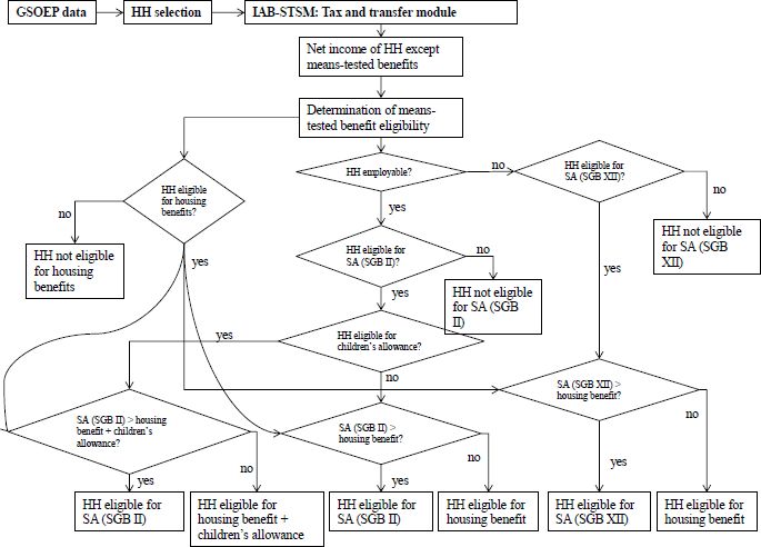

Simulation of welfare entitlements in the IAB-STSM.
Source: Bruckmeier and Wiemers (2011).
Note that according to Table 5 we expect many of the utility proxy variables to have an impact on the cost of take-up as well. In some cases (e.g., “single parents” or “disabled head of household”) the assumed effect on information and/or stigma costs works in the same direction as the effects on utility. In the case of single parents we assume lower stigma costs, since single parents may perceive themselves as being more needy than couples, who can share the burden of work and childcare. For this reason we expect these variables to have an unambiguous impact on the likelihood of take-up. This is not the case for variables like “age” or “qualification”, implying that we are agnostic about the sign of these coefficients. Additional variables, which should mainly be related to the costs of claiming SA, are “sex of the head of household” (higher social stigma for males), “area of living” (rural or metropolitan relative to intermediate area, where stigma in rural areas should be higher because of higher social control), a dummy for living in eastern Germany and for home owners. We hypothesize a positive relationship between living in eastern Germany and the degree and duration of needs, which should mainly reflect a worse labor market situation than in western Germany. Home owners, on the other hand, are likely to need SA for a shorter period than non-owners, if the earning potential of owners is higher on average. At the same time, a home owner’s fear of being forced to sell her home may detain her from claiming SA. We are agnostic about the impact of the migrant dummies on the take-up decision. Migrants – on average – have a higher degree of needs, but at the same time face higher information costs (language barriers). The last column of Table 5 shows the overall expected effect of the variables on the probability of claiming SA.
Proxy variables of utility and costs and their expected effect on the probability of claiming SA.
| Utility from SA | Claiming costs | Effect | |||
|---|---|---|---|---|---|
| Degree of needs | Duration of needs | Inform. costs | Stigma/fear | ||
| Calculated monthly benefit (cont.) | + | + | |||
| Singles (ref.: couple without children) | + | + | + | ||
| Single parent (ref.: couple without children) | + | + | − | + | |
| Family with children (ref.: couple without children) | + | + | ? | ||
| Number of children aged < = 3 years | + | + | + | ||
| Number of children aged > 14 years | − | − | − | ||
| HHH retired | + | + | + | ? | |
| Disability of HHH | + | + | − | + | |
| High qualif. HHH (ref.: med. qual.) | − | − | ? | ||
| Low qualif. HHH (ref.: med. qual.) | + | + | ? | ||
| Age, age2 of HHH | + | + | + | ? | |
| Male HHH | + | − | |||
| Home owner household | − | + | − | ||
| Rural area (ref.: interm. area) | + | + | + | ? | |
| Metropolitan area (ref.: interm. area) | − | − | − | ? | |
| Eastern Germany | + | + | + | ||
| EU migrants | + | + | + | + | ? |
| Non-EU migrants | + | + | + | + | ? |
| Migrants with German citizenship | + | + | + | + | ? |
-
Note: Column “effect” indicates the expected effect of the respective variable on the probability of claiming SA. A “+” sign in the utility columns corresponds to a positive expected effect on the probability of take-up, while a “+” sign in the cost columns has the opposite effect (vice versa for “-” signs). A “?” stands for an ambiguous overall effect. “HH” stands for household.
-
Source: Based on Bruckmeier and Wiemers (2011).
D. Means of the covariates for eligible households
Means of covariates used in the regression by take-up status, pooled sample 2005–2011.
| Non-take-up-households | Take-up-households | |
|---|---|---|
| Calculated monthly benefit (in €) | 292 | 662*** |
| Singles | 0.56 | 0 44*** |
| Single parents | 0.12 | 0.21*** |
| Family with children | 0.10 | 0.16*** |
| Number of children aged < = 3 years | 0.07 | 0.15*** |
| Number of children aged > 14 years | 0.16 | 0.24*** |
| HHH retired | 0.18 | 0.08*** |
| Disability of HHH | 0.02 | 0.02 |
| High qualif. HHH (ref.: interm. qual.) | 0.22 | 0.08*** |
| Low qualif. HHH (ref.: interm. qual.) | 0.23 | 0.31*** |
| Age | 43.38 | 44.60*** |
| Male HHH | 0.43 | 0.43 |
| Home owner household | 0.18 | 0.07*** |
| Rural area (ref.: interm. area) | 0.12 | 0.15*** |
| Metropolitan area (ref.: interm. area) | 0.40 | 0.39 |
| Eastern Germany | 0.31 | 0.46*** |
| EU Migrants | 0.03 | 0.02** |
| Non-EU-Migrants | 0.07 | 0.09* |
| Migrants with German citizenship | 0.19 | 0.20 |
| Dummy 2006 | 0.17 | 0.17 |
| Dummy 2007 | 0.16 | 0.16 |
| Dummy 2008 | 0.16 | 0.14* |
| Dummy 2009 | 0.13 | 0.15 |
| Dummy 2010 | 0.11 | 0.11 |
| Dummy 2011 | 0.13 | 0.16 |
| Sample size | 2810 | 3150 |
-
Source: GSOEP, authors’ own computations based on IAB-STSM. Stars denote rejection of the E-test on equal means of non-take-up vs. take-up households with the significance levels.
-
*
p < 0.1.
-
**
p < 0.05.
-
***
p < 0.01. HHH = head of household. The sample sizes add up to the number of observations used in the take-up estimations, 5960.
E. Reform effects for alternative estimation models
Effects of changing social assistance by 100 € per month on finances and caseloads for different assumptions on take-up. Simulation of endogenous take-up based on pooled probit.
| Change monthly SA by | +100 € | −100 € | ||||
|---|---|---|---|---|---|---|
| Take-up | 100% TU | ETU | ETU | 100% TU | ETU | ETU |
| Share of sunk costs | N/A | 0 | 1 | N/A | 0 | 1 |
| Caseloads (HH in 1,000) | ||||||
| Social assistance | +1,222 | +639 | +591 | −1,143 | −623 | −346 |
| Housing benefit | −506 | −329 | −331 | +856 | +540 | +533 |
| Enh. child benefit | −87 | −87 | −87 | +118 | +118 | +118 |
| Annual costs in m € | ||||||
| Social assistance (base amount) | +6,540 | +6,490 | +6,433 | −5,112 | −5,036 | −4,558 |
| Social assistance (housing) | +4,654 | +3,318 | +3,169 | −4,221 | −3,210 | −2,053 |
| Housing benefit | −449 | −350 | −353 | +1,350 | +1,027 | +1,028 |
| Enh. child benefit | −220 | −220 | −220 | +405 | +405 | +405 |
| Total effect in m € | +10,525 | +9,238 | +9,029 | −7,578 | −6,814 | −5,178 |
-
Notes: A negative sign for the annual total fiscal effect implies a budget surplus.
-
HH = households, TU = take-up, ETU = endogenous take-up.
-
Source: Own calculations based on SOEP 2005–2011.
Effects of changing social assistance by 100 € per month on finances and caseloads for different assumptions on take-up. Simulation of endogenous take-up based on RE probit.
| Change monthly SA by | +100 € | −100 € | ||||
|---|---|---|---|---|---|---|
| Take-up | 100% TU | ETU | ETU | 100% TU | ETU | ETU |
| Share of sunk costs | N/A | 0 | 1 | N/A | 0 | 1 |
| Caseloads (HH in 1,000) | ||||||
| Social assistance | +1,222 | +637 | +620 | −1,143 | −561 | −344 |
| Housing benefit | −506 | −335 | −337 | +856 | +561 | +557 |
| Enh. child benefit | −87 | −87 | −87 | +118 | +118 | +118 |
| Annual costs in m € | ||||||
| Social assistance (base amount) | +6,540 | +6,326 | +6,305 | −5,112 | −4,915 | −4,512 |
| Social assistance (housing) | +4,654 | +3,246 | +3,190 | −4,221 | −2,925 | −2,003 |
| Housing benefit | −449 | −355 | −357 | +1,350 | +1,028 | +1,029 |
| Enh. child benefit | −220 | −220 | −220 | +405 | +405 | +405 |
| Total effect in m € | +10,525 | +8,997 | +8,918 | −7,578 | −6,407 | −5,081 |
-
Notes: A negative sign for the annual total fiscal effect implies a budget surplus.
-
HH = households, TU = take-up, ETU = endogenous take-up.
-
Source: Own calculations based on SOEP 2005–2011.
References
-
1
Arbeitsangebot-seffekte und Verteilungswirkungen der Hartz-IV-ReformIAB Forschungsbericht.
-
2
Nicht-Inanspruchnahme zustehender Sozialhilfeleistungen (Dunkelzif ferstudie) - Endbericht zur Studie im Auftrag des Bundesministeriums für Gesundheit und Soziale SicherungBerlin: Edition Sigma.
-
3
Förderung Existenz sichernder Beschäftigung im NiedriglohnbereichIAB Forschungsbericht.
-
4
Modelling the Take-up of Means-Tested Benefits: The Case of Housing Benefits in the United KingdomEconomic Journal 98:58–74.
-
5
Did Working Families’ Tax Credit Work? The Impact of In-work Support on Labour Supply in Great BritainLabour Economics 13:699–720.
-
6
Simulationsrechnungen zum Ausmaβ der Nicht-Inanspruchnahme von Leistungen der GrundsicherungIAB-Forschungsbericht.
-
7
A New Targeting - A New Take-Up? Non-Take-Up of Social Assistance in Germany after Social Policy Reforms. IAB Discussion Paper No. 10/2011Nuremberg: Institute for Employment Research.
- 8
- 9
-
10
To Claim or Not to Claim: Estimating NonTake-Up of Social Assistance in Germany and the Role of Measurement Error. SOEP Papers on Multidisciplinary Panel Data Research, No. 53 DIWOctober, To Claim or Not to Claim: Estimating NonTake-Up of Social Assistance in Germany and the Role of Measurement Error. SOEP Papers on Multidisciplinary Panel Data Research, No. 53 DIW, Berlin.
-
11
The Take-Up of Supplementary Benefit: Gaps in the ‘Safety Net’?Fiscal Studies 8:1–14.
- 12
-
13
The Take-Up of Multiple Means-Tested Benefits by British Pensioners: Evidence from the Family Resources SurveyFiscal studies 25:279–303.
-
14
What Should Be the Role of Means-testing in State Pensions?Department of Health and Human Sciences, University of Essex.
-
15
Dokumentation des Steuer-Transfer-Mikrosimulationsmodells STSM - Version 1995-1999Dokumentation Nr. 03-06, Zentrum für Europäische Wirtschafts-forschung.
-
16
Labour Supply and Welfare Participation in Australian Two-Adult Households: Accounting for Involuntary Unemployment and the ‘Cost’ of Part-time Work (Tech. Rep.)Centre of Policy Studies/IMPACT Centre: Monash University.
-
17
Take It or Leave It: (Non-)Take-Up Behavior of Social Assistance in GermanyJournal of Applied Social Science Studies 121:27–58.
-
18
A Structural Model of Multiple Welfare Program Participation and Labor SupplyInternational Economic Review 39:553–589.
-
19
Amemiya’s Generalized Least Squares and Tests of Overidentification in Simultaneous Equation Models with Qualitative or Limited Dependent VariablesEconometric Reviews 11:319–328.
- 20
-
21
Simulating the Reform of Means-tested Benefits with Endogenous Take-up and Claim CostsOxford Bulletin of Economics and Statistics 68:135–166.
-
22
Rational Poverty of Poor Rationality? - The Take-up of Social Assistance Benefits379–398, Review of Income and Wealth, 47, 3, Review of Income and Wealth.
-
23
Non-Take-Up of Social Security Benefits in EuropeJournal of European Social Policy 1:15–30.
-
24
The German Socio-Economic Panel Study (SOEP)-Scope, Evolution and EnhancementJournal of Applied Social Studies 127:139–169.
- 25
-
26
Forecasting Behavioural and Distributional Effects of the Bofinger-Walwei Model Using MicrosimulationJahrbiicherfur Nationalokonomie und Statistik 229:492–511.
-
27
Nichtinanspruchnahme von Sozialhilfe - Eine empirische Analyse des Unerwarteten347–373, Jahrbiicher für Nationalokonomie und Statistik, 225, 3, Volk- swirtschaftliche Diskussionsbeitrage No. 31, Wirtschaftswissenschaftliche Fakultat, Martin- Luther-Universitat Halle-Wittenberg.
Article and author information
Author details
Acknowledgements
I would like to thank the editor of this journal and two anonymous referees for their helpful comments.
Publication history
- Version of Record published: August 31, 2015 (version 1)
Copyright
© 2015, Wiemers
This article is distributed under the terms of the Creative Commons Attribution License, which permits unrestricted use and redistribution provided that the original author and source are credited.