Endogenizing take-up of social assistance in a microsimulation model a case study for Germany
- Institute for Employment Research (IAB), Germany
- Article
- Figures and data
- Jump to
Figures

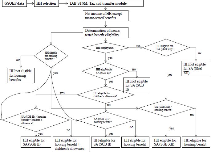
Simulation of welfare entitlements in the IAB-STSM.
Source: Bruckmeier and Wiemers (2011).
Tables
Rates of non-take-up of social assistance 2005–2011
| Non-take-up Rate | 95%-Confidence Interval | |
|---|---|---|
| 2005 | 48.0 | [43.6–52.5] |
| 2006 | 42.6 | [38.6–46.6] |
| 2007 | 40.8 | [36.7–44.9] |
| 2008 | 45.3 | [40.7–49.9] |
| 2009 | 38.6 | [33.8–43.4] |
| 2010 | 38.8 | [33.4–44.1] |
| 2011 | 42.8 | [37.8–47.8] |
| Pooled | 42.4 | [40.7–44.1] |
-
Weighted non -take-up rates in percent. Source: GSOEP years 2005–2011, pooled data, IAB-STSM
Marginal effects on probability of take-up (dependent variable).
| Model 1 Probit | Model 2 IV Probit | Model 3 RE Probit | |
|---|---|---|---|
| Simulated monthly benefit (in 100 EUR) | .0718*** | .0627*** | .0745*** |
| (.0016) | (.0062) | (.0023) | |
| Single | .0463*** | .0444*** | .0278 |
| (.0144) | (.0150) | (.0244) | |
| Single parent | .0529** | .0780*** | .0506 |
| (.0217) | (.0277) | (.0358) | |
| Family with children | .0112 | .0353 | .0123 |
| (.0242) | (.0299) | (.0371) | |
| Number of children aged < = 3 years | .0545*** | .0699** | .0696** |
| (.0205) | (.0230) | (.0289) | |
| Number of children age > 14 years | −.0410*** | −.0345** | −.0360* |
| (.0124) | (.0138) | (.0184) | |
| HHH retired | −.0161 | −.0528* | .0063 |
| (.0195) | (.0306) | (.0315) | |
| Disability of HHH | .0579 | .0588 | .1059** |
| (.0385) | (.0402) | (.0522) | |
| High qualif. HHH (ref.: med. qual.) | −.1322*** | −.1375*** | −.1824*** |
| (.0158) | (.0168) | (.0271) | |
| Low qualif. HHH (ref.: med. qual.) | .0302** | .0420*** | .0568*** |
| (.0128) | (.0151) | (.0216) | |
| Age of HHH | .0045*** | .0053*** | .0042*** |
| (.0004) | (.0007) | (.0007) | |
| Male HHH | .0233** | .0310** | .0371** |
| (.0110) | (.0124) | (.0187) | |
| Home owner household | −.1715*** | −.1961*** | −.2275*** |
| (.0166) | (.0224) | (.0280) | |
| Rural area (ref.: interm. area) | .0369** | .0367** | .0437 |
| (.0155) | (.0162) | (.0272) | |
| Metrop. area (ref.: interm. area) | −.0016 | −.0002 | −.0039 |
| (.0111) | (.0116) | (.0186) | |
| Eastern Germany | .1375*** | .1447*** | .1816*** |
| (.0115) | (.0126) | (.0200) | |
| EU migrants | −.0946*** | −.1035*** | −.0594 |
| (.0347) | (.0374) | (.0626) | |
| Non-EU migrants | .0111 | .0199 | .0323 |
| (.0215) | (.0231) | (.0365) | |
| Migrants with German citizenship | .0114 | .0156 | .0213 |
| (.0137) | (.0147) | (.0223) | |
| Observations | 5960 | 5960 | 5960 |
| Wald test of exogeneity: 㱲2(1) | 2.88* | ||
| (Pseudo)log-likelihood | −2749.99 | −17327.596 | −2369.8414 |
| ρ | .717 |
-
Source: GSOEP 2005–2011, own calculations. HHH stands for head of household. Wave-dummies included in all models. Standard errors in parentheses.
-
*
p < 0.1.
-
**
p < 0.05.
-
***
p < 0.01.
Effects of changing social assistance by 100 € per month on finances and caseloads for different assumptions on take-up. Simulation of endogenous take-up based on pooled IV probit.
| Change monthly SA by | + 100 € | −100 € | ||||
|---|---|---|---|---|---|---|
| Take-up | 100% TU | ETU | ETU | 100% TU | ETU | ETU |
| Share of sunk costs | N/A | 0 | 1 | N/A | 0 | 1 |
| Caseloads (HH in 1,000) | ||||||
| Social assistance | +1,222 | +600 | +581 | −1,143 | −528 | −333 |
| Housing benefit | −506 | −336 | −338 | +856 | +561 | +558 |
| Enh. child benefit | −87 | −87 | −87 | +118 | +118 | +118 |
| Annual costs in m € | ||||||
| Social assistance (base amount) | +6,540 | +6,184 | +6,157 | −5,112 | −4,852 | −4,467 |
| Social assistance (housing) | +4,654 | +3,054 | +2,990 | −4,221 | −2,784 | −1,945 |
| Housing benefit | −449 | −356 | −358 | +1,350 | +1,029 | +1,029 |
| Enh. child benefit | −220 | −220 | −220 | +405 | +405 | +405 |
| Total effect in m € | +10,525 | +8,662 | +8,569 | −7,578 | −6,202 | −4,978 |
-
Notes: A negative sign for the annual total fiscal effect implies a budget surplus.
HH = households, TU = take-up, ETU = endogenous take-up.
-
Source: Own calculations based on SOEP 2005–2011.
Components of net household income in the IAB-STSM.
| Income components | Determined in tax and transfer module? | ||
|---|---|---|---|
| 1 | Earned income | no | |
| + | Self-employed income | no | |
| + | Capital income | no | |
| + | Rental income | no | |
| + | Other incomes (pensions) | no | |
| 2 | − | Social security contributions | yes |
| − | Income tax | yes | |
| − | Alimony payments | yes | |
| 3 | + | Child benefit | yes |
| + | Child-raising allowance | yes | |
| + | Unemployment benefits | yesa | |
| + | Federal student support, stipends, claims to maintenance, widow’s allowance, maternity allowance, reduced hours compensation | no | |
| 4 | + | Housing allowance | yes |
| + | Children’s allowance | yes | |
| + | Social assistance for employable persons (SGB II) | yes | |
| + | Social assistance for unemployable persons (SGB XII) | yes | |
| = | Net household income | yes |
-
a
Endogenous if labor supply reactions are considered. Otherwise we use reported unemployment benefits.
Source: Bruckmeier and Wiemers(2011).
Proxy variables of utility and costs and their expected effect on the probability of claiming SA.
| Utility from SA | Claiming costs | Effect | |||
|---|---|---|---|---|---|
| Degree of needs | Duration of needs | Inform. costs | Stigma/fear | ||
| Calculated monthly benefit (cont.) | + | + | |||
| Singles (ref.: couple without children) | + | + | + | ||
| Single parent (ref.: couple without children) | + | + | − | + | |
| Family with children (ref.: couple without children) | + | + | ? | ||
| Number of children aged < = 3 years | + | + | + | ||
| Number of children aged > 14 years | − | − | − | ||
| HHH retired | + | + | + | ? | |
| Disability of HHH | + | + | − | + | |
| High qualif. HHH (ref.: med. qual.) | − | − | ? | ||
| Low qualif. HHH (ref.: med. qual.) | + | + | ? | ||
| Age, age2 of HHH | + | + | + | ? | |
| Male HHH | + | − | |||
| Home owner household | − | + | − | ||
| Rural area (ref.: interm. area) | + | + | + | ? | |
| Metropolitan area (ref.: interm. area) | − | − | − | ? | |
| Eastern Germany | + | + | + | ||
| EU migrants | + | + | + | + | ? |
| Non-EU migrants | + | + | + | + | ? |
| Migrants with German citizenship | + | + | + | + | ? |
-
Note: Column “effect” indicates the expected effect of the respective variable on the probability of claiming SA. A “+” sign in the utility columns corresponds to a positive expected effect on the probability of take-up, while a “+” sign in the cost columns has the opposite effect (vice versa for “-” signs). A “?” stands for an ambiguous overall effect. “HH” stands for household.
-
Source: Based on Bruckmeier and Wiemers (2011).
Means of covariates used in the regression by take-up status, pooled sample 2005–2011.
| Non-take-up-households | Take-up-households | |
|---|---|---|
| Calculated monthly benefit (in €) | 292 | 662*** |
| Singles | 0.56 | 0 44*** |
| Single parents | 0.12 | 0.21*** |
| Family with children | 0.10 | 0.16*** |
| Number of children aged < = 3 years | 0.07 | 0.15*** |
| Number of children aged > 14 years | 0.16 | 0.24*** |
| HHH retired | 0.18 | 0.08*** |
| Disability of HHH | 0.02 | 0.02 |
| High qualif. HHH (ref.: interm. qual.) | 0.22 | 0.08*** |
| Low qualif. HHH (ref.: interm. qual.) | 0.23 | 0.31*** |
| Age | 43.38 | 44.60*** |
| Male HHH | 0.43 | 0.43 |
| Home owner household | 0.18 | 0.07*** |
| Rural area (ref.: interm. area) | 0.12 | 0.15*** |
| Metropolitan area (ref.: interm. area) | 0.40 | 0.39 |
| Eastern Germany | 0.31 | 0.46*** |
| EU Migrants | 0.03 | 0.02** |
| Non-EU-Migrants | 0.07 | 0.09* |
| Migrants with German citizenship | 0.19 | 0.20 |
| Dummy 2006 | 0.17 | 0.17 |
| Dummy 2007 | 0.16 | 0.16 |
| Dummy 2008 | 0.16 | 0.14* |
| Dummy 2009 | 0.13 | 0.15 |
| Dummy 2010 | 0.11 | 0.11 |
| Dummy 2011 | 0.13 | 0.16 |
| Sample size | 2810 | 3150 |
-
Source: GSOEP, authors’ own computations based on IAB-STSM. Stars denote rejection of the E-test on equal means of non-take-up vs. take-up households with the significance levels.
-
*
p < 0.1.
-
**
p < 0.05.
-
***
p < 0.01. HHH = head of household. The sample sizes add up to the number of observations used in the take-up estimations, 5960.
Effects of changing social assistance by 100 € per month on finances and caseloads for different assumptions on take-up. Simulation of endogenous take-up based on pooled probit.
| Change monthly SA by | +100 € | −100 € | ||||
|---|---|---|---|---|---|---|
| Take-up | 100% TU | ETU | ETU | 100% TU | ETU | ETU |
| Share of sunk costs | N/A | 0 | 1 | N/A | 0 | 1 |
| Caseloads (HH in 1,000) | ||||||
| Social assistance | +1,222 | +639 | +591 | −1,143 | −623 | −346 |
| Housing benefit | −506 | −329 | −331 | +856 | +540 | +533 |
| Enh. child benefit | −87 | −87 | −87 | +118 | +118 | +118 |
| Annual costs in m € | ||||||
| Social assistance (base amount) | +6,540 | +6,490 | +6,433 | −5,112 | −5,036 | −4,558 |
| Social assistance (housing) | +4,654 | +3,318 | +3,169 | −4,221 | −3,210 | −2,053 |
| Housing benefit | −449 | −350 | −353 | +1,350 | +1,027 | +1,028 |
| Enh. child benefit | −220 | −220 | −220 | +405 | +405 | +405 |
| Total effect in m € | +10,525 | +9,238 | +9,029 | −7,578 | −6,814 | −5,178 |
-
Notes: A negative sign for the annual total fiscal effect implies a budget surplus.
-
HH = households, TU = take-up, ETU = endogenous take-up.
-
Source: Own calculations based on SOEP 2005–2011.
Effects of changing social assistance by 100 € per month on finances and caseloads for different assumptions on take-up. Simulation of endogenous take-up based on RE probit.
| Change monthly SA by | +100 € | −100 € | ||||
|---|---|---|---|---|---|---|
| Take-up | 100% TU | ETU | ETU | 100% TU | ETU | ETU |
| Share of sunk costs | N/A | 0 | 1 | N/A | 0 | 1 |
| Caseloads (HH in 1,000) | ||||||
| Social assistance | +1,222 | +637 | +620 | −1,143 | −561 | −344 |
| Housing benefit | −506 | −335 | −337 | +856 | +561 | +557 |
| Enh. child benefit | −87 | −87 | −87 | +118 | +118 | +118 |
| Annual costs in m € | ||||||
| Social assistance (base amount) | +6,540 | +6,326 | +6,305 | −5,112 | −4,915 | −4,512 |
| Social assistance (housing) | +4,654 | +3,246 | +3,190 | −4,221 | −2,925 | −2,003 |
| Housing benefit | −449 | −355 | −357 | +1,350 | +1,028 | +1,029 |
| Enh. child benefit | −220 | −220 | −220 | +405 | +405 | +405 |
| Total effect in m € | +10,525 | +8,997 | +8,918 | −7,578 | −6,407 | −5,081 |
-
Notes: A negative sign for the annual total fiscal effect implies a budget surplus.
-
HH = households, TU = take-up, ETU = endogenous take-up.
-
Source: Own calculations based on SOEP 2005–2011.