Regression-style models for parameter estimation in dynamic microsimulation: An empirical performance assessment
- Centre of Methods and Policy Application in the Social Sciences, The University of Auckland, New Zealand
- Article
- Figures and data
- Jump to
Figures
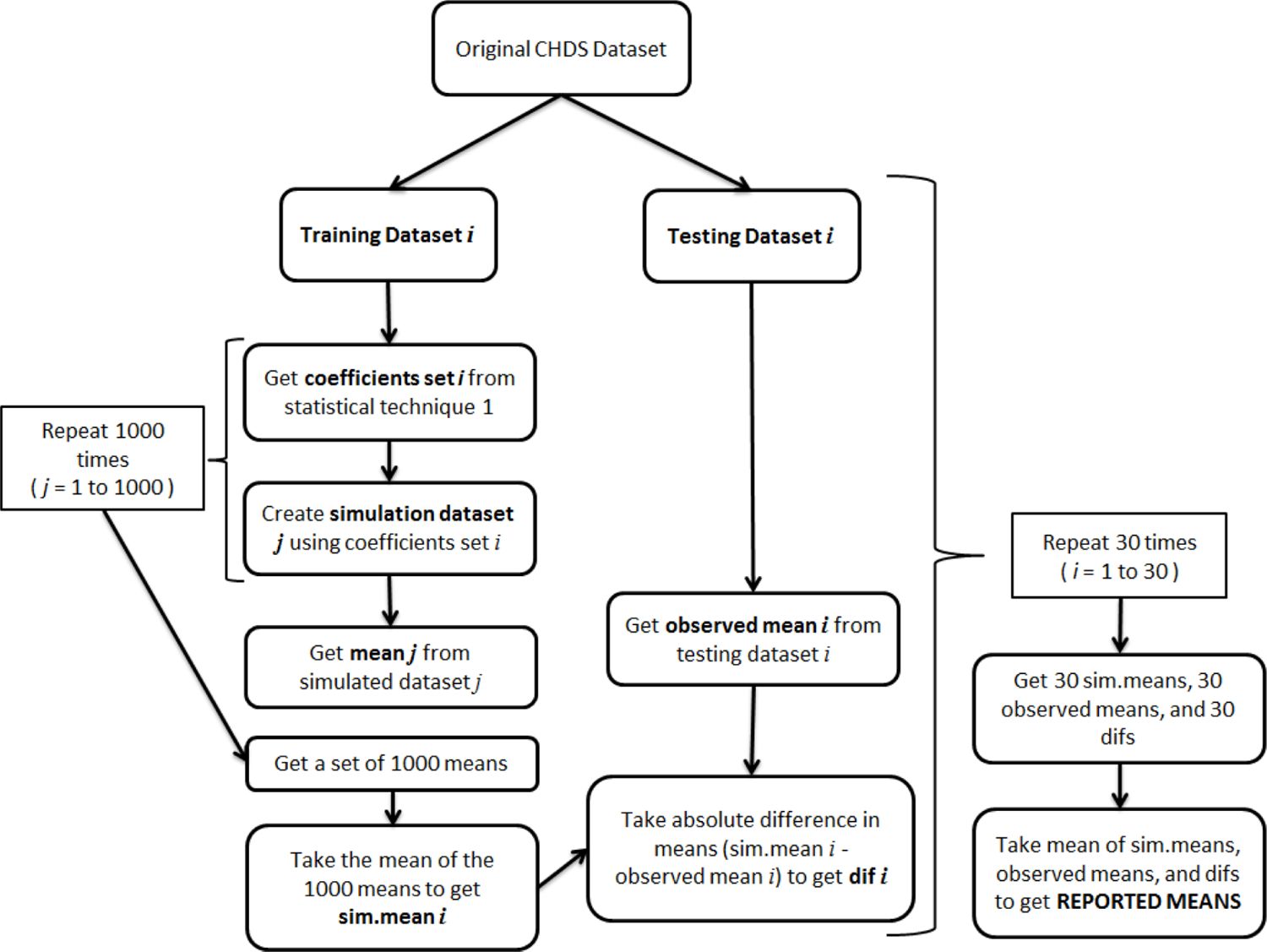
Flowchart showing the cross validation method used to calculate the simulated means, observed means, and the mean absolute differences reported in the results.

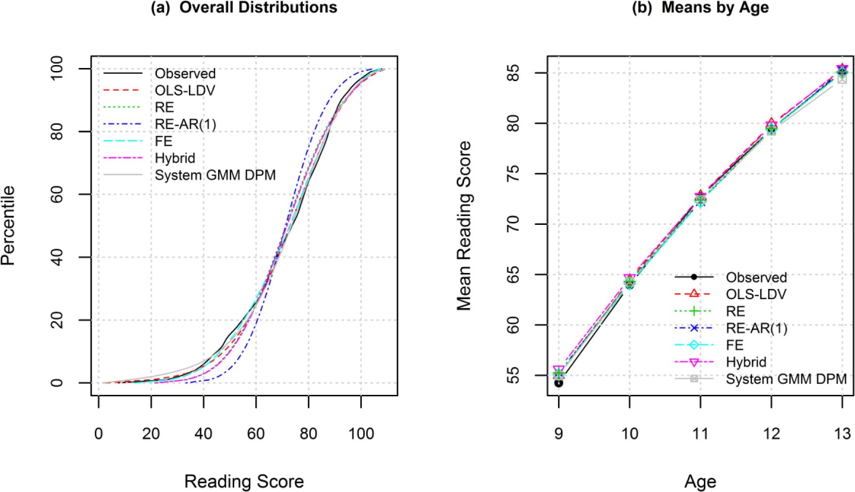
Comparison of the observed reading scores and the reading scores simulated under the six models.
(a) Cumulative distribution curves for the overall distributions.
(b) Means by age.

Cumulative distribution curves of the observed reading scores and the reading scores simulated under the six models.
(a) Child-specific correlations of current and lagged score
(b) Child-specific standard deviations.

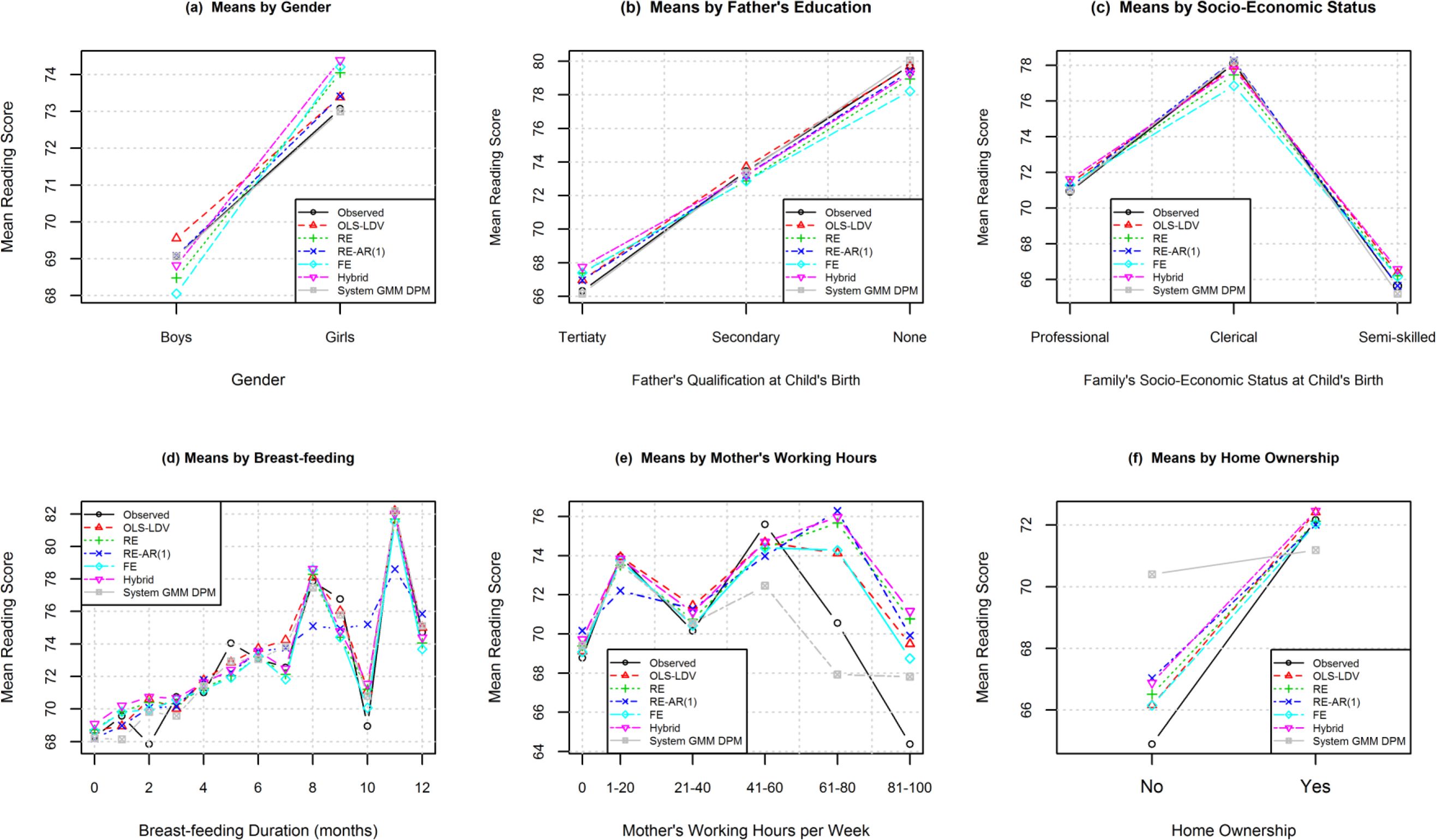
Comparison of observed and simulated mean reading scores by predictors.
(a) By gender. (b) By father's education. (c) By socio-economic status. (d) By breast-feeding. (e) By mother's working hours. (f) By home-ownership. Lines joining points are added to make distinctions between models more clear.
Tables
Statistical regression techniques used by other dynamic microsimulation models (Table legend).
| OLS regression with an LVD | Random effects | Fixed effects |
|---|---|---|
| MINT3: Earnings of retirees who choose to work, earnings of social security beneficiaries (Toder et al., 2002) | PenSim2: Earnings (Emmerson, Reed, & Shephard, 2004) | MINT1: Earnings (Toder et al., 2002) |
| SVERIGE: Earnings (Rephann & Holm, 2004) | MIDAS: Hours worked, wages (Dekkers et al., 2008) | Income Distribution of the Dutch Elderly: Income (Knoef, Alessie, & Kalwij, 2013) |
| DYNAMOD-2: Earnings (Bækgaard, 2002) | DYNASIM-3: Hours worked, earnings (Favreault & Smith, 2004) | MINT3: Pre-retirement earnings after age 50 (Toder et al., 2002) |
| LifePaths: Hours worked (Wolfson, 1995) | SAGE: Earnings (Zaidi et al., 2009) | |
| MINT3: Non-pension wealth, home equity, non-pension assets (Toder et al., 2002) | ||
| SESIM: Earnings, interest paid, size of loan (Klevmarken & Lindgren, 2008) |
Predictors used in the regression models.
| Variable | Categories/description |
|---|---|
| Time-invariant Predictors | Values available only at the child’s birth |
| Gender | Male; Female |
| Mother’s education | No formal qualifications; Secondary qualification; Tertiary qualification |
| Father’s education | No formal qualifications, Secondary qualification; Tertiary qualification |
| Family’s socio-economic position | Semi-skilled, Unskilled, unemployed; Clerical, technical, skilled; Professional, managerial |
| Based on the Elley-Irving scale (Elley & Irving, 1976) | |
| Breast-feeding | Duration in months |
| Time-variant Predictors | Values available at each year |
| LDV | The lagged dependent variable; The value of the reading score at the previous year |
| Child’s age | 8 to 13 years |
| Mother’s hours worked | The average number of hours of paid work performed per week by the mother/mother figure |
| Home ownership | Owned or mortgaged; Rented |
| Father’s smoking | The average number of cigarettes smoked per day by the father/father figure |
Assumptions made for each model. ✓A indicates that the assumption is made by the model. Following this may be either the result of testing for the assumption or a comment (A dash (-) indicates that the test is not relevant).
| Assumption | Test used | OLS-LDV | RE | RE-AR(1) | FE | HYBRID | GMM Dynamic Panel | |
|---|---|---|---|---|---|---|---|---|
| 1 | No individual effects: μi = 0, εi,t = υi,t | LR test for non-zero , p-value based on a mixture of chi-squares (COVTEST in the GLIMMIX procedure, SAS 9.3). | ✓ A, LDV in model: x2(1) = 0.00, p = .9999; LDV not in model: x2(1) = 7958, p < .0001 | - | - | - | - | - |
| 2 | Individual effects independent of within-child errors: Cov(μi, υi,t = 0 | Test for Pearson’s correlation between estimated individual effectsa and residuals | - | ✓A, , p < .0001 | ✓A, , p < .0001 | |||
| 3 | Individual effects independent of each other: μi~iid | Assumed by virtue of the individuals being randomly selected and from different families | - | ✓A | ✓A | μis eliminated by transformation | ✓A | μis eliminated by transformation |
| 4 | μi~N(0.σb) | Shapiro-Wilk test on the empirical BLUPsb of individual effects | - | ✓A, W = 0.99, p = .0001, but plotting shows distribution close to normal | ✓A, W = 0.99, p < .0001, but plotting shows distribution close to normal | ✓A, W = 0.99, p = .0001, but plotting shows distribution close to normal | ||
| 5 | Cross-sectional ‘between’ effects equal to within ‘fixed’ ,, . K = λ effects: k = λ | Hausman test | ✓A, x2(5) = 2.55, p = .7693 | ✓A, x2(5) = 2.55, p = .7693 | ✓A, x2(5) = 2.55, p = .7693 | Only λ estimated | λ and κ estimated separately | Only λ estimated |
| 6 | Exogenous time-invariant predictors (TIPs): Cov(υi,t, xi,t) = 0, Cov(zi, υi,t) = 0, | C statistic from endogtest in stata’s ivreg2c | ✓A, null of exogeneity not rejected for any TIPsd. LDV endogenous by definition. | ✓A, null of exogeneity rejected for most TIPse | ✓A, no convenient test – refer to tests for RE model | TIPs not used | ✓A, null of exogeneity rejected for half of the TIPse | Diff GMM: TIPs not used. System GMM: Assumption does not need to be made |
| 7 | Exogenous time-variant predictors (TVPs): Cov(εi,t, xi,t) = 0, Cov(μi, ) = 0 | C statistic from endogtest in stata’s ivreg2 or xtivreg2c | ✓A, null of exogeneity rejected for one TVPd | ✓A, null of exogeneity rejected for two TVPse | ✓A, no convenient test – refer to tests for RE model | ✓A, null of exogeneity not rejected for any TVPsf | ✓A, null of exogeneity rejected for one TVPe | Assumption does not need to be madeg |
| 8 | υi,t~iid N(0, σ2): Within-child errors serially uncorrelated | System GMM: Arellano-Bond test for AR in first differences Other models: xtserial in stata (Wooldridge 2002) | ✓A, F(1, 1003) = 398.5, p < .0001 | ✓A, F(1, 1043) = 115.5, p < .0001 | Assumes an AR(1) structureh | ✓A, F(1, 1043) = 115.5, p < .0001 | ✓A, F(1, 1043) = 115.5, p < .0001 | Assumption not made but choice of instruments depends on degree of serial correlation. instruments depends on degree of serial correlation. AR(2): z = 4.33, p < .0001. AR(3): z = -1.60, p = .109. |
| 9 | υi,t~iid N(0, σ2) Within-child errors independent across individuals (no cross-sectional dependence) | Pesaran’s test (Pesaran 2004): xtcsd in stata | - | ✓A, statistic = 6.62, p < .0001 | ✓A, no convenient test – refer to test for RE model | ✓A, statistic = 6.45, p < .0001 | ✓A, no convenient test – refer to tests for RE and FE models | ✓A, no convenient test – refer to tests for RE and FE models |
| 10 | Validity of moment conditions (validity of instruments) for Difference GMM | Hansen test | - | - | - | - | - | ✓A, x2(22) = 24.47, p = .323 |
| 11 | Validity of additional moment conditions for System GMM | Difference in Hansen test | - | - | - | - | - | ✓A, x2(4)=16.27, p=.003 |
| 12 | Stationarity of within-child errors | Hadri and Larsson (2005) | Z = -2.80, p = .0051 | Z = 19.31, p < .0001 | Z = 19.46, p < .0001 | Z = 19.34, p < .0001 | Z = 19.32, p < .0001 | System GMM: Z = -2.80, p = .0051 |
-
a
Estimated individual effects were the empirical BLUPs (best linear unbiased predictors) estimated by SAS
-
b
BLUP = best linear unbiased predictor. Empirical BLUPs estimated in SAS by requesting fitted values with and without BLUPS and taking the difference.
-
c
The tests utilised additional variables not included in any models as excluded instruments (each tested for exogeneity and relevance). Predictors were tested individually with all other variables in the model treated as exogenous. Each model was checked for identification and weak. Significance was set at the .05 level. Full results of the tests and stata code are available in the online Appendix.
-
d
LDV included in the model. cluster option not used (panel data structure ignored).
-
e
LDV not included in the model. cluster option used to indicate panel data structure.
-
f
LDV not included in the model. cluster option used to indicate panel data structure. fe option used.
-
g
Although the exogeneity if variables should be investigated so that the analyst has some indication of what variables need to be instrumented and which do not.
-
h
A test for whether the AR(1) structure was defensible compared to an unstructured structure was attempted in SAS but the model with the unstructured model would not converge
Mean absolute differences (MAD) (smaller is better) and standardised mean absolute differences (SMAD) (more negative is better) between simulated and observed data.
| Data characteristic | OLS – LDV | RE) | RE-AR(1) | FE | HYBRID | SYSTEM GMM | |||||||
|---|---|---|---|---|---|---|---|---|---|---|---|---|---|
| MAD | SMAD | MAD | SMAD | MAD | SMAD | MAD | SMAD | MAD | SMAD | MAD | SMAD | ||
| PRESS statistica | 0.53 | −0.11 | 0.44 | −0.66 | 0.81 | 1.59 | 0.39 | −0.99 | 0.44 | −0.64 | 0.68 | 0.80 | |
| Overall distributions | 1.47 | −0.97 | 2.66 | 0.07 | 4.70 | 1.86 | 2.08 | −0.44 | 2.69 | 0.10 | 1.87 | −0.62 | |
| Means across time | 0.50 | −1.42 | 0.69 | −0.05 | 0.70 | −0.01 | 0.73 | 0.23 | 0.93 | 1.66 | 0.64 | −0.41 | |
| Child-specific correlations (dynamism) | 0.09 | −1.45 | 0.23 | 0.85 | 0.24 | 0.92 | 0.15 | −0.46 | 0.23 | 0.82 | 0.14 | −0.68 | |
| Child-specific standard deviations | 0.76 | −1.75 | 1.07 | −0.27 | 1.38 | 1.19 | 1.16 | 0.14 | 1.13 | 0.02 | 1.27 | 0.66 | |
| Time invariant predictors: | |||||||||||||
| Gender | 0.72 | −1.51 | 1.16 | 0.19 | 1.15 | 0.15 | 1.38 | 1.02 | 1.37 | 0.98 | 0.90 | −0.82 | |
| Breast-feeding | 1.69 | −0.77 | 1.82 | −0.42 | 2.74 | 1.97 | 1.77 | −0.57 | 1.97 | −0.04 | 1.92 | −0.17 | |
| Father’s education | 0.85 | −1.64 | 1.19 | −0.15 | 1.51 | 1.18 | 1.38 | 0.64 | 1.34 | 0.47 | 1.11 | −0.51 | |
| Mother’s education | 0.91 | −1.46 | 1.29 | −0.04 | 1.68 | 1.43 | 1.35 | 0.19 | 1.45 | 0.56 | 1.12 | −0.67 | |
| Family’s socio-economic status | 0.94 | −1.49 | 1.06 | −0.72 | 1.38 | 1.36 | 1.21 | 0.28 | 1.25 | 0.56 | 1.17 | 0.01 | |
| Time-variant predictors: | |||||||||||||
| Home-ownership | 1.07 | −0.64 | 1.29 | −0.45 | 1.60 | −0.18 | 1.20 | −0.53 | 1.57 | −0.21 | 4.19 | 2.01 | |
| Mother’s hours worked | 4.81 | −0.61 | 4.95 | −0.49 | 7.88 | 1.86 | 4.63 | −0.75 | 5.01 | −0.44 | 6.10 | 0.43 | |
| Father’s smoking | 5.31 | −0.80 | 5.73 | −0.51 | 8.42 | 1.36 | 5.34 | −0.78 | 5.80 | −0.46 | 8.17 | 1.19 | |
| Weighted means | |||||||||||||
| Scheme 1b | −1.11 | −0.11 | 1.11 | −0.27 | 0.30 | 0.08 | |||||||
| Scheme 2c | −1.12 | −0.07 | 1.11 | −0.28 | 0.34 | 0.02 | |||||||
-
a
The PRESS statistic is not a mean absolute difference but a standardised measure of the distance between the observed and predicted values. Smaller values are better.
-
b
Time-invariant predictors given a weight of 1/5 each, time-variant predictors given a weight of 1/3 each. Other characteristics each given a weight of 1.
-
c
Means by predictor variables given a combined weight of 1 with the time-invariant predictors each given a weight of 0.1 and the time-variant predictors each given a weight of 1/6. Other characteristics each given a weight of 1.
Overall weighted mean of the standardised mean absolute differences (using weighting scheme 1a) by age for each model.
| AGE | MEAN OVER AGEb | |||||
|---|---|---|---|---|---|---|
| MODEL | 9 | 10 | 11 | 12 | 13 | |
| OLS – LDV | −1.11 | −1.10 | −1.10 | −1.06 | −1.04 | −1.11 |
| RE | −0.08 | −0.07 | −0.06 | −0.11 | −0.11 | −0.11 |
| RE-AR (1) | 1.22 | 1.18 | 1.09 | 0.94 | 0.74 | 1.11 |
| FE | −0.16 | −0.24 | −0.27 | −0.30 | −0.27 | −0.27 |
| Hybrid | 0.42 | 0.34 | 0.28 | 0.28 | 0.24 | 0.30 |
| System GMM | −0.29 | −0.09 | 0.05 | 0.25 | 0.44 | 0.08 |
-
a
Time-invariant predictors given a weight of 1/5 each, time-variant predictors given a weight of 1/3 each. Other characteristics each given a weight of 1.
-
b
The weighted mean of the SMADs that were averaged over age. This is the same value as shown in the second-to-last row of Table 4.
Coefficients and standard errors estimated on the full dataset for each of the techniques.
| Variable | OLS – LDV | RE | RE-AR(1) | FE | Hybrid | System GMM DPM 2 Step a | System GMM DPM 1 Step a | |
|---|---|---|---|---|---|---|---|---|
| Reading score previous centred (LDV) | 0.90 | 0.83 | 0.82 | |||||
| (0.01) | (0.04) | (0.04) | ||||||
| Reading score previous centred squared (LDV squared) | −0.00 | −0.01 | −0.01 | |||||
| (0.00) | (0.00) | (0.00) | ||||||
| Child’s age centred | −0.33 | 8.02 | 7.98 | 8.01 | 8.02 | 0.23 | 0.27 | |
| (0.09) | (0.05) | (0.10) | (0.05) | (0.05) | (0.41) | (0.41) | ||
| Child’s age centred squared | 0.13 | −0.52 | −0.06 | −0.51 | −0.52 | −0.01 | −0.02 | |
| (0.04) | (0.03) | (0.03) | (0.03) | (0.03) | (0.10) | (0.10) | ||
| Gender (reference: Female) | 0.07 | −3.78 | −3.31 | −3.79 | 0.51 | 0.49 | ||
| (0.21) | (0.98) | (0.75) | (0.98) | (0.34) | (0.35) | |||
| Father’s education (reference: No formal education) | Tertiary | 1.43 | 6.78 | 5.10 | 6.54 | 0.68 | 0.51 | |
| (0.39) | (1.79) | (1.37) | (1.81) | (0.58) | (0.57) | |||
| Secondary | 0.98 | 4.60 | 3.57 | 4.56 | 0.67 | 0.71 | ||
| (0.25) | (1.18) | (0.90) | (1.18) | (0.36) | (0.36) | |||
| Mother’s education (reference: No formal education) | Tertiary | 1.01 | 7.02 | 5.16 | 6.76 | 1.18 | 1.05 | |
| (0.32) | (1.53) | (1.17) | (1.55) | (0.55) | (0.54) | |||
| Secondary | 0.42 | 2.47 | 1.65 | 2.31 | 0.47 | 0.40 | ||
| (0.26) | (1.21) | (0.92) | (1.21) | (0.37) | (0.35) | |||
| Family’s socio-economic status (reference: Semi-skilled) | Professional | 0.22 | 4.28 | 3.37 | 3.76 | 0.71 | 0.22 | |
| (0.39) | (1.79) | (1.37) | (1.82) | (0.72) | (0.77) | |||
| Clerical | 0.03 | 2.43 | 1.97 | 2.02 | 0.18 | −0.14 | ||
| (0.27) | (1.23) | (0.93) | (1.25) | (0.54) | (0.56) | |||
| Breast-feeding | 0.07 | 0.26 | 0.20 | 0.25 | 0.05 | 0.06 | ||
| (0.03) | (0.13) | (0.10) | (0.13) | (0.03) | (0.03) | |||
| 0.00 | 0.01 | 0.00 | 0.01 | (D, M): 0.01, 0.01 | −0.02 | 0.01 | ||
| Mother’s hours worked | (0.01) | (0.01) | (0.01) | (0.01) | (0.01), (0.04) | (0.04) | (0.04) | |
| Father’s smoking | 0.00 | −0.03 | −0.01 | −0.03 | (D, M): -0.02, -0.09 | −0.16 | −0.24 | |
| (0.01) | (0.02) | (0.02) | (0.02) | (0.02), (0.07) | (0.12) | (0.11) | ||
| Home-ownership (reference: owned/mortgaged) | −0.72 | −1.48 | −1.15 | −1.30 | (D, M): -1.31, -3.75 | 3.66 | 2.29 | |
| (0.30) | (0.43) | (0.42) | (0.44) | (0.45), (1.62) | (2.98) | (3.18) | ||
-
D: For the hybrid technique, estimate of the within / fixed effect calculated from the deviation variable.
-
M: For the hybrid technique, estimate of the between/cross-sectional effect calculated from the mean variable.
-
a
Windmeijer corrected standard errors are displayed
Mean absolute differences (MAD) (smaller is better) and standardised mean absolute differences (SMAD) (more negative is better) between simulated and observed data for age 9.
| OLS-LDV | RE | RE-AR (1) | Hybrid | FE | System GMM DPM | |||||||
|---|---|---|---|---|---|---|---|---|---|---|---|---|
| Data Characteristic | MAD | SMAD | MAD | SMAD | MAD | SMAD | MAD | SMAD | MAD | SMAD | MAD | SMAD |
| PRESS statistica | 0.26 | −0.65 | 0.35 | −0.21 | 0.79 | 2.01 | 0.35 | −0.19 | 0.31 | −0.43 | 0.28 | −0.53 |
| Overall distributions | 1.50 | −0.64 | 1.86 | −0.43 | 5.96 | 2.01 | 2.10 | −0.28 | 2.28 | −0.18 | 1.78 | −0.48 |
| Means across time | 0.50 | −1.42 | 0.69 | −0.05 | 0.70 | −0.01 | 0.93 | 1.66 | 0.73 | 0.23 | 0.64 | −0.41 |
| Within-child correlations (dynamism) | 0.09 | −1.45 | 0.23 | 0.85 | 0.24 | 0.92 | 0.23 | 0.82 | 0.15 | −0.46 | 0.14 | −0.68 |
| Within-child standard deviations | 0.76 | −1.75 | 1.07 | −0.27 | 1.38 | 1.19 | 1.13 | 0.02 | 1.16 | 0.14 | 1.27 | 0.66 |
| Time-invariant predictors: | ||||||||||||
| Gender | 0.82 | −1.06 | 1.13 | 0.03 | 1.28 | 0.57 | 1.54 | 1.47 | 1.17 | 0.16 | 0.79 | −1.17 |
| Breast-feading | 1.39 | −0.71 | 1.57 | −0.35 | 2.69 | 1.90 | 1.90 | 0.31 | 1.47 | −0.55 | 1.45 | −0.6 |
| Father’s education | 0.40 | −1.24 | 1.23 | −0.03 | 1.60 | 1.09 | 1.51 | 0.82 | 1.41 | 0.52 | 0.87 | −1.16 |
| Mother’s education | 0.90 | −1.1 | 1.28 | 0.02 | 1.71 | 1.30 | 1.56 | 0.85 | 1.30 | 0.09 | 0.88 | −1.17 |
| Family’s socio-economic status | 0.92 | −1.17 | 1.26 | −0.02 | 1.56 | 1.03 | 1.58 | 1.11 | 1.32 | 0.19 | 0.93 | −1.14 |
| Time-variant predictors: | ||||||||||||
| Home-ownership | 1.02 | −1.13 | 1.34 | −0.38 | 1.40 | −0.23 | 1.75 | 0.57 | 1.27 | −0.54 | 2.23 | 1.71 |
| Mother’s hours worked | 3.79 | −0.56 | 4.05 | −0.35 | 7.03 | 2.03 | 4.17 | −0.26 | 3.85 | −0.51 | 4.05 | −0.35 |
| Father’s smoking | 3.56 | −0.79 | 4.39 | −0.31 | 8.32 | 1.98 | 4.52 | −0.24 | 3.97 | −0.55 | 4.79 | −0.08 |
| Weighted means | ||||||||||||
| Scheme 1b | −1.11 | −0.08 | 1.22 | 0.42 | −0.16 | −0.29 | −1.11 | |||||
| Scheme 2c | −1.14 | −0.05 | 1.22 | 0.42 | −0.15 | −0.29 | −1.14 | |||||
-
a
The PRESS statistic is not a mean absolute difference but a standardised measure of the distance between the observed and predicted values. Smaller values are better.
-
b
Time-invariant predictors given a weight of 1/5 each, time-variant predictors given a weight of 1/3 each. Other characteristics were each given a weight of 1.
-
c
Means by predictor variables given a combined weight of 1 with the time-invariant predictors each given a weight of 0.1 and the time-variant predictors each given a weight of 1/6. Other characteristics were each given a weight of 1.
Mean absolute differences (MAD) (smaller is better) and standardised mean absolute differences (SMAD) (more negative is better) between simulated and observed data for age 10.
| OLS-LDV | RE | RE-AR (1) | Hybrid | FE | System GMM DPM | |||||||
|---|---|---|---|---|---|---|---|---|---|---|---|---|
| Data Characteristic | MAD | SMAD | MAD | SMAD | MAD | SMAD | MAD | SMAD | MAD | SMAD | MAD | SMAD |
| PRESS statistica | 0.41 | −0.31 | 0.38 | −0.48 | 0.81 | 1.94 | 0.39 | −0.46 | 0.32 | −0.82 | 0.49 | 0.12 |
| Overall distributions | 1.46 | −0.83 | 2.77 | −0.07 | 6.25 | 1.95 | 2.85 | −0.02 | 1.96 | −0.54 | 2.04 | −0.49 |
| Means across time | 0.50 | −1.42 | 0.69 | −0.05 | 0.70 | −0.01 | 0.93 | 1.66 | 0.64 | 0.23 | 0.73 | −0.41 |
| Within-child correlations (dynamism) | 0.09 | −1.45 | 0.23 | 0.85 | 0.24 | 0.92 | 0.23 | 0.82 | 0.14 | −0.46 | 0.15 | −0.68 |
| Within-child standard deviations | 0.76 | −1.75 | 1.07 | −0.27 | 1.38 | 1.19 | 1.13 | 0.02 | 1.27 | 0.14 | 1.16 | 0.66 |
| Time-invariant predictors: | ||||||||||||
| Gender | 0.66 | −1.26 | 1.05 | 0.15 | 1.11 | 0.4 | 1.32 | 1.14 | 1.21 | 0.74 | 0.69 | −1.17 |
| Breast-feading | 1.49 | −0.88 | 1.77 | −0.26 | 2.75 | 1.93 | 1.94 | 0.12 | 1.68 | −0.45 | 1.67 | −0.46 |
| Father’s education | 0.79 | −1.49 | 1.26 | 0.03 | 1.57 | 1.04 | 1.44 | 0.6 | 1.47 | 0.72 | 0.97 | −0.91 |
| Mother’s education | 0.78 | −1.4 | 1.35 | 0.2 | 1.70 | 1.18 | 1.54 | 0.71 | 1.40 | 0.33 | 0.92 | −1.01 |
| Family’s socio-economic status | 0.78 | −1.46 | 1.06 | −0.21 | 1.35 | 1.08 | 1.28 | 0.75 | 1.26 | 0.65 | 0.92 | −0.82 |
| Time-variant predictors: | ||||||||||||
| Home-ownership | 0.77 | −0.67 | 0.97 | −0.47 | 1.24 | −0.19 | 1.29 | −0.15 | 0.92 | −0.52 | 3.42 | 2.00 |
| Mother’s hours worked | 4.67 | −0.58 | 4.77 | −0.49 | 7.44 | 1.88 | 4.88 | −0.39 | 4.45 | −0.78 | 5.72 | 0.35 |
| Father’s smoking | 4.29 | −0.81 | 4.80 | −0.49 | 8.23 | 1.71 | 4.83 | −0.47 | 4.52 | −0.67 | 6.68 | 0.72 |
| Weighted means | ||||||||||||
| Scheme 1b | −1.10 | −0.07 | 1.18 | 0.34 | −0.24 | −0.09 | ||||||
| Scheme 2c | −1.12 | −0.04 | 1.19 | 0.36 | −0.26 | −0.12 | ||||||
-
a
The PRESS statistic is not a mean absolute difference but a standardised measure of the distance between the observed and predicted values. Smaller values are better.
-
b
Time-invariant predictors given a weight of 1/5 each, time-variant predictors given a weight of 1/3 each. Other characteristics were each given a weight of 1.
-
c
Means by predictor variables given a combined weight of 1 with the time-invariant predictors each given a weight of 0.1 and the time-variant predictors each given a weight of 1/6. Other characteristics were each given a weight of 1.
Mean absolute differences (MAD) (smaller is better) and standardised mean absolute differences (SMAD) (more negative is better) between simulated and observed data for age 11.
| OLS-LDV | RE | RE-AR (1) | Hybrid | FE | System GMM DPM | |||||||
|---|---|---|---|---|---|---|---|---|---|---|---|---|
| Data Characteristic | MAD | SMAD | MAD | SMAD | MAD | SMAD | MAD | SMAD | MAD | SMAD | MAD | SMAD |
| PRESS statistica | 0.54 | −0.01 | 0.43 | −0.65 | 0.82 | 1.55 | 0.43 | −0.65 | 0.36 | −1.05 | 0.69 | 0.81 |
| Overall distributions | 1.87 | −0.93 | 3.70 | 0.2 | 6.32 | 1.81 | 3.67 | 0.18 | 2.37 | −0.63 | 2.37 | −0.63 |
| Means across time | 0.50 | −1.42 | 0.69 | −0.05 | 0.70 | −0.01 | 0.93 | 1.66 | 0.73 | 0.23 | 0.64 | −0.41 |
| Within-child correlations (dynamism) | 0.09 | −1.45 | 0.23 | 0.85 | 0.24 | 0.92 | 0.23 | 0.82 | 0.15 | −0.46 | 0.14 | −0.68 |
| Within-child standard deviations | 0.76 | −1.75 | 1.07 | −0.27 | 1.38 | 1.19 | 1.13 | 0.02 | 1.16 | 0.14 | 1.27 | 0.66 |
| Time-invariant predictors: | ||||||||||||
| Gender | 0.57 | −1.5 | 1.13 | 0.27 | 1.14 | 0.33 | 1.26 | 0.71 | 1.38 | 1.11 | 0.76 | −0.92 |
| Breast-feading | 1.84 | −1 | 2.14 | −0.22 | 2.99 | 1.93 | 2.21 | −0.04 | 2.10 | −0.32 | 2.09 | −0.35 |
| Father’s education | 0.83 | −1.58 | 1.33 | 0.07 | 1.65 | 1.08 | 1.40 | 0.29 | 1.57 | 0.85 | 1.09 | −0.71 |
| Mother’s education | 0.93 | −1.4 | 1.65 | 0.3 | 1.97 | 1.07 | 1.72 | 0.48 | 1.79 | 0.63 | 1.06 | −1.08 |
| Family’s socio-economic status | 0.86 | −1.66 | 1.06 | −0.57 | 1.38 | 1.22 | 1.22 | 0.31 | 1.26 | 0.55 | 1.19 | 0.16 |
| Time-variant predictors: | ||||||||||||
| Home-ownership | 1.04 | −0.79 | 1.57 | −0.4 | 2.16 | 0.04 | 1.78 | −0.24 | 1.34 | −0.57 | 4.71 | 1.96 |
| Mother’s hours worked | 5.17 | −0.45 | 5.06 | −0.52 | 8.79 | 1.9 | 5.13 | −0.48 | 4.70 | −0.76 | 6.35 | 0.31 |
| Father’s smoking | 5.42 | −0.88 | 5.90 | −0.51 | 8.22 | 1.26 | 5.96 | −0.47 | 5.65 | −0.70 | 8.27 | 1.30 |
| Weighted means | ||||||||||||
| Scheme 1b | −1.10 | −0.06 | 1.09 | 0.28 | −0.27 | 0.05 | ||||||
| Scheme 2c | −1.10 | −0.03 | 1.09 | 0.34 | −0.30 | 0.01 | ||||||
-
a
The PRESS statistic is not a mean absolute difference but a standardised measure of the distance between the observed and predicted values. Smaller values are better.
-
b
Time-invariant predictors given a weight of 1/5 each, time-variant predictors given a weight of 1/3 each. Other characteristics were each given a weight of 1.
-
c
Means by predictor variables given a combined weight of 1 with the time-invariant predictors each given a weight of 0.1 and the time-variant predictors each given a weight of 1/6. Other characteristics were each given a weight of 1.
Mean absolute differences (MAD) (smaller is better) and standardised mean absolute differences (SMAD) (more negative is better) between simulated and observed data for age 12.
| OLS-LDV | RE | RE-AR (1) | Hybrid | FE | System GMM DPM | |||||||
|---|---|---|---|---|---|---|---|---|---|---|---|---|
| Data Characteristic | MAD | SMAD | MAD | SMAD | MAD | SMAD | MAD | SMAD | MAD | SMAD | MAD | SMAD |
| PRESS statistica | 0.65 | 0.19 | 0.48 | −0.74 | 0.82 | 1.05 | 0.48 | −0.73 | 0.42 | −1.06 | 0.86 | 1.29 |
| Overall distributions | 2.00 | −1.1 | 3.72 | 0.37 | 5.23 | 1.66 | 3.68 | 0.33 | 2.61 | −0.58 | 2.48 | −0.69 |
| Means across time | 0.50 | −1.42 | 0.69 | −0.05 | 0.70 | −0.01 | 0.93 | 1.66 | 0.73 | 0.23 | 0.64 | −0.41 |
| Within-child correlations (dynamism) | 0.09 | −1.45 | 0.23 | 0.85 | 0.24 | 0.92 | 0.23 | 0.82 | 0.15 | −0.46 | 0.14 | −0.68 |
| Within-child standard deviations | 0.76 | −1.75 | 1.07 | −0.27 | 1.38 | 1.19 | 1.13 | 0.02 | 1.16 | 0.14 | 1.27 | 0.66 |
| Time-invariant predictors: | ||||||||||||
| Gender | 0.78 | −1.49 | 1.18 | 0.18 | 1.09 | −0.18 | 1.31 | 0.76 | 1.45 | 1.33 | 0.99 | −0.61 |
| Breast-feading | 1.92 | −0.62 | 1.95 | −0.52 | 2.76 | 1.94 | 2.06 | −0.19 | 1.88 | −0.73 | 2.17 | 0.13 |
| Father’s education | 0.92 | −1.71 | 1.16 | −0.37 | 1.46 | 1.25 | 1.25 | 0.11 | 1.33 | 0.56 | 1.26 | 0.16 |
| Mother’s education | 1.03 | −1.57 | 1.31 | −0.22 | 1.67 | 1.53 | 1.42 | 0.33 | 1.38 | 0.11 | 1.32 | −0.18 |
| Family’s socio-economic status | 1.04 | −1.09 | 1.01 | −1.32 | 1.26 | 0.97 | 1.17 | 0.16 | 1.18 | 0.27 | 1.26 | 1.01 |
| Time-variant predictors: | ||||||||||||
| Home-ownership | 1.44 | −0.49 | 1.51 | −0.44 | 1.75 | −0.29 | 1.76 | −0.29 | 1.38 | −0.52 | 5.43 | 2.03 |
| Mother’s hours worked | 5.14 | −0.57 | 5.30 | −0.44 | 8.14 | 1.82 | 5.29 | −0.44 | 4.78 | −0.85 | 6.45 | 0.48 |
| Father’s smoking | 7.48 | −0.71 | 7.80 | −0.48 | 9.13 | 0.51 | 7.86 | −0.43 | 7.49 | −0.71 | 10.88 | 1.82 |
| Weighted means | ||||||||||||
| Scheme 1b | −1.06 | −0.11 | 0.94 | 0.28 | −0.30 | 0.25 | ||||||
| Scheme 2c | −1.08 | −0.05 | 0.95 | 0.34 | −0.32 | 0.16 | ||||||
-
a
The PRESS statistic is not a mean absolute difference but a standardised measure of the distance between the observed and predicted values. Smaller values are better.
-
b
Time-invariant predictors given a weight of 1/5 each, time-variant predictors given a weight of 1/3 each. Other characteristics were each given a weight of 1.
-
c
Means by predictor variables given a combined weight of 1 with the time-invariant predictors each given a weight of 0.1 and the time-variant predictors each given a weight of 1/6. Other characteristics were each given a weight of 1.
Mean absolute differences (MAD) (smaller is better) and standardised mean absolute differences (SMAD) (more negative is better) between simulated and observed data for age 13.
| OLS-LDV | RE | RE-AR (1) | Hybrid | FE | System GMM DPM | |||||||
|---|---|---|---|---|---|---|---|---|---|---|---|---|
| Data Characteristic | MAD | SMAD | MAD | SMAD | MAD | SMAD | MAD | SMAD | MAD | SMAD | MAD | SMAD |
| PRESS statistica | 0.78 | 0.25 | 0.56 | −0.75 | 0.83 | 0.5 | 0.56 | −0.73 | 0.52 | −0.93 | 1.08 | 1.66 |
| Overall distributions | 1.98 | −1.43 | 3.82 | 0.6 | 4.39 | 1.23 | 3.78 | 0.56 | 3.20 | −0.09 | 2.49 | −0.87 |
| Means across time | 0.50 | −1.42 | 0.69 | −0.05 | 0.7 | −0.01 | 0.93 | 1.66 | 0.73 | 0.23 | 0.64 | −0.41 |
| Within-child correlations (dynamism) | 0.09 | −1.45 | 0.23 | 0.85 | 0.24 | 0.92 | 0.23 | 0.82 | 0.15 | −0.46 | 0.14 | −0.68 |
| Within-child standard deviations | 0.76 | −1.75 | 1.07 | −0.27 | 1.38 | 1.19 | 1.13 | 0.02 | 1.16 | 0.14 | 1.27 | 0.66 |
| Time-invariant predictors: | ||||||||||||
| Gender | 0.74 | −1.65 | 1.32 | 0.22 | 1.12 | −0.42 | 1.40 | 0.48 | 1.68 | 1.36 | 1.26 | 0.01 |
| Breast-feading | 1.81 | −0.38 | 1.68 | −0.75 | 2.52 | 1.67 | 1.73 | −0.61 | 1.69 | −0.72 | 2.21 | 0.78 |
| Father’s education | 0.86 | −1.39 | 0.98 | −0.72 | 1.27 | 0.81 | 1.11 | −0.06 | 1.12 | −0.01 | 1.37 | 1.37 |
| Mother’s education | 0.93 | −0.62 | 0.87 | −0.85 | 1.36 | 1.08 | 1.01 | −0.27 | 0.89 | −0.78 | 1.45 | 1.43 |
| Family’s socio-economic status | 1.09 | −0.26 | 0.89 | −1.08 | 1.32 | 0.74 | 1.01 | −0.57 | 1.03 | −0.48 | 1.54 | 1.63 |
| Time-variant predictors: | ||||||||||||
| Home-ownership | 1.07 | −0.48 | 1.07 | −0.48 | 1.46 | −0.24 | 1.28 | −0.36 | 1.09 | −0.47 | 5.15 | 2.03 |
| Mother’s hours worked | 5.27 | −0.79 | 5.57 | −0.56 | 7.98 | 1.3 | 5.60 | −0.54 | 5.40 | −0.69 | 7.95 | 1.27 |
| Father’s smoking | 5.79 | −0.51 | 5.75 | −0.53 | 8.22 | 0.7 | 5.83 | −0.5 | 5.07 | −0.88 | 10.23 | 1.71 |
| Weighted means | ||||||||||||
| Scheme 1b | −1.06 | −0.11 | 0.94 | 0.28 | −0.30 | 0.25 | ||||||
| Scheme 2c | −1.08 | −0.05 | 0.95 | 0.34 | −0.32 | 0.16 | ||||||
-
a
The PRESS statistic is not a mean absolute difference but a standardised measure of the distance between the observed and predicted values. Smaller values are better.
-
b
Time-invariant predictors given a weight of 1/5 each, time-variant predictors given a weight of 1/3 each. Other characteristics were each given a weight of 1.
-
c
Means by predictor variables given a combined weight of 1 with the time-invariant predictors each given a weight of 0.1 and the time-variant predictors each given a weight of 1/6. Other characteristics were each given a weight of 1.
t-values from paired t-tests (df=29) comparing the absolute differences (between the simulated and observed percentiles of the distribution of reading scores). Values greater than 2.46 indicate (unadjusted) significance at the .01 level.
| Percentile | |||||
|---|---|---|---|---|---|
| Comparison | 10th | 25th | 50th | 75th | 90th |
| OLS-LDV – RE | −31.08 | −19.56 | −28.23 | −24.00 | −14.27 |
| OLS-LDV – RE-AR(1) | −9.90 | −18.06 | −17.57 | −8.52 | −6.81 |
| OLS-LDV – Hybrid | −2.11 | 0.11 | 2.12 | −1.35 | −0.61 |
| OLS-LDV – System GMM DPM | 1.45 | −10.74 | −22.55 | −7.51 | −8.31 |
| OLS-LDV – FE | −29.93 | −9.64 | −6.25 | −29.91 | −13.54 |
| RE – RE-AR(1) | −2.63 | −2.30 | 1.66 | 1.75 | −3.02 |
| RE – Hybrid | 2.41 | 9.73 | 25.19 | 8.85 | 2.46 |
| RE – System GMM DPM | 11.01 | −0.14 | 12.25 | 9.27 | −2.54 |
| RE – FE | 20.03 | 9.72 | 3.66 | 31.28 | 10.41 |
| RE-AR(1) – Hybrid | 14.97 | 13.80 | 27.01 | 22.03 | 10.03 |
| RE-AR(1) – System GMM DPM | 30.17 | 5.88 | 14.38 | 26.04 | 10.18 |
| RE-AR(1) – FE | 3.34 | 10.18 | 16.87 | 6.51 | 3.00 |
| Hybrid – System GMM DPM | 11.02 | 0.92 | 5.88 | 5.89 | 0.31 |
| Hybrid – FE | 2.72 | −8.57 | −18.00 | −4.00 | −3.29 |
| System GMM DPM – FE | −31.08 | −19.56 | −28.23 | −24.00 | −14.27 |
t-values from paired t-tests (df=29) comparing the absolute differences (between the simulated and observed means of reading scores). Values greater than 2.46 indicate (unadjusted) significance at the .01 level.
| Age | |||||
|---|---|---|---|---|---|
| Comparison | 9 | 10 | 11 | 12 | 13 |
| OLS-LDV – RE | −1.84 | −1.95 | −3.48 | −0.90 | −1.83 |
| OLS-LDV – RE-AR(1) | −1.85 | −1.65 | −3.75 | −1.04 | −2.31 |
| OLS-LDV – Hybrid | −3.39 | −3.59 | −4.38 | −3.43 | −3.07 |
| OLS-LDV – System GMM DPM | 1.80 | 0.21 | −2.02 | −1.49 | −2.69 |
| OLS-LDV – FE | −1.53 | −2.34 | −3.70 | −1.38 | −2.05 |
| RE – RE-AR(1) | −0.05 | 1.98 | −1.10 | −0.28 | −0.74 |
| RE – Hybrid | −3.47 | −2.94 | −1.75 | −2.64 | −1.98 |
| RE – System GMM DPM | 2.16 | 2.12 | 1.38 | −0.77 | −1.75 |
| RE – FE | 0.96 | −0.75 | −1.87 | −1.57 | −1.15 |
| RE-AR(1) – Hybrid | −3.43 | −3.13 | −1.32 | −2.44 | −1.72 |
| RE-AR(1) – System GMM DPM | 2.18 | 1.80 | 1.68 | −0.71 | −1.56 |
| RE-AR(1) – FE | 0.91 | −1.55 | −1.12 | −1.07 | −0.38 |
| Hybrid – System GMM DPM | 3.65 | 3.63 | 2.56 | 1.05 | −0.76 |
| Hybrid – FE | 3.54 | 2.09 | 0.78 | 1.79 | 1.16 |
| System GMM DPM – FE | −1.85 | −2.38 | −2.02 | 0.29 | 1.52 |
t-values from paired t-tests (df = 29) comparing the absolute differences (between the simulated and observed percentiles of the distribution of child-specific correlations between current and lagged reading scores). Values greater than 2.46 indicate (unadjusted) significance at the .01 level.
| Percentile | |||||
|---|---|---|---|---|---|
| Comparison | 10th | 25th | 50th | 75th | 90th |
| OLS-LDV – RE | −37.88 | −82.01 | −93.94 | −89.52 | −83.17 |
| OLS-LDV – RE-AR(1) | −30.27 | −44.09 | −55.95 | −62.67 | −61.41 |
| OLS-LDV – Hybrid | −40.68 | −88.06 | −96.87 | −87.17 | −78.17 |
| OLS-LDV – System GMM DPM | −14.53 | −13.64 | −13.83 | −13.49 | −12.42 |
| OLS-LDV – FE | −14.39 | −83.70 | −111.84 | −104.30 | −95.05 |
| RE – RE-AR(1) | −14.68 | 0.23 | 22.05 | 40.07 | 47.60 |
| RE – Hybrid | 2.32 | 2.40 | 2.45 | 2.49 | 2.21 |
| RE – System GMM DPM | 3.64 | 33.06 | 65.29 | 75.15 | 72.97 |
| RE – FE | 52.68 | 51.85 | 49.02 | 46.74 | 44.81 |
| RE-AR(1) – Hybrid | 14.35 | 0.36 | −18.04 | −30.84 | −34.43 |
| RE-AR(1) – System GMM DPM | 10.04 | 25.17 | 40.75 | 48.78 | 49.55 |
| RE-AR(1) – FE | 34.24 | 24.66 | 14.86 | 4.77 | −2.32 |
| Hybrid – System GMM DPM | 3.50 | 34.37 | 69.56 | 75.74 | 71.70 |
| Hybrid – FE | 51.39 | 48.19 | 44.55 | 41.19 | 37.90 |
| System GMM DPM – FE | 9.43 | −14.40 | −47.04 | −63.95 | −67.09 |
t-values from paired t-tests (df = 29) comparing the absolute differences (between the simulated and observed percentiles of the distribution of within-child standard deviations of reading scores). Values greater than 2.46 indicate (unadjusted) significance at the .01 level.
| Percentile | |||||
|---|---|---|---|---|---|
| Comparison | 10th | 25th | 50th | 75th | 90th |
| OLS-LDV – RE | −9.99 | −7.43 | −7.45 | 10.71 | 7.70 |
| OLS-LDV – RE-AR(1) | 6.32 | 1.89 | −12.79 | −22.29 | −17.18 |
| OLS-LDV – Hybrid | −10.20 | −7.87 | −7.97 | 9.05 | 8.06 |
| OLS-LDV – System GMM DPM | −8.23 | −5.83 | −1.88 | −11.14 | −13.73 |
| OLS-LDV – FE | −9.84 | −5.31 | −2.92 | 0.78 | −0.01 |
| RE – RE-AR(1) | 41.95 | 42.88 | −23.07 | −24.19 | −15.65 |
| RE – Hybrid | −2.70 | −2.81 | −2.74 | −4.01 | 0.82 |
| RE – System GMM DPM | 3.10 | 2.52 | 6.10 | −16.29 | −15.82 |
| RE – FE | −0.02 | 9.12 | 9.48 | −5.53 | −19.46 |
| RE-AR(1) – Hybrid | −31.43 | −22.63 | 8.32 | 24.63 | 16.44 |
| RE-AR(1) – System GMM DPM | −10.40 | −6.09 | 11.37 | 6.68 | 4.14 |
| RE-AR(1) – FE | −35.78 | −26.65 | 20.58 | 9.90 | 8.05 |
| Hybrid – System GMM DPM | 3.54 | 3.13 | 6.71 | −14.82 | −16.49 |
| Hybrid – FE | 2.17 | 7.17 | 8.74 | −3.88 | −13.89 |
| System GMM DPM – FE | −3.12 | −0.91 | −1.21 | 6.90 | 6.82 |
t-values from paired t-tests (df = 29) comparing the absolute differences (between the simulated and observed mean reading scores by gender). Values greater than 2.46 indicate (unadjusted) significance at the .01 level.
| Gender | ||
|---|---|---|
| Comparison | Girls | Boyx |
| OLS-LDV – RE | −3.97 | −3.21 |
| OLS-LDV – RE-AR(1) | −3.75 | −4.12 |
| OLS-LDV – Hybrid | −4.51 | −3.65 |
| OLS-LDV – System GMM DPM | −2.48 | −1.64 |
| OLS-LDV – FE | −5.08 | −4.03 |
| RE – RE-AR(1) | 0.97 | −0.91 |
| RE – Hybrid | −2.88 | −0.98 |
| RE – System GMM DPM | 2.22 | 1.52 |
| RE – FE | −3.70 | −3.81 |
| RE-AR(1) – Hybrid | −2.44 | 0.07 |
| RE-AR(1) – System GMM DPM | 1.71 | 2.30 |
| RE-AR(1) – FE | −2.16 | −0.98 |
| Hybrid – System GMM DPM | 3.35 | 1.85 |
| Hybrid – FE | 1.12 | −1.13 |
| System GMM DPM – FE | −3.41 | −2.84 |
t-values from paired t-tests (df = 29) comparing the absolute differences (between the simulated and observed mean reading scores by duration of breast-feeding). Values greater than 2.46 indicate (unadjusted) significance at the .01 level.
| Breast-feeding Duration (months) | |||||
|---|---|---|---|---|---|
| Comparison | 0 | 3 | 6 | 9 | 12 |
| OLS-LDV – RE | −0.35 | −2.91 | −1.63 | −5.11 | −0.45 |
| OLS-LDV – RE-AR(1) | −2.99 | −4.71 | −3.66 | −4.12 | −3.40 |
| OLS-LDV – Hybrid | −2.15 | −2.66 | −2.87 | −4.09 | −1.10 |
| OLS-LDV – System GMM DPM | −2.89 | −2.52 | −2.01 | −4.44 | −1.10 |
| OLS-LDV – FE | −0.33 | −2.46 | −2.96 | −4.79 | −0.96 |
| RE – RE-AR(1) | −3.08 | −3.82 | −3.46 | −0.95 | −2.69 |
| RE – Hybrid | −2.76 | −1.43 | −2.58 | 3.03 | −1.26 |
| RE – System GMM DPM | −2.07 | −0.09 | −0.91 | 0.93 | −0.09 |
| RE – FE | −0.04 | −0.12 | −2.42 | 0.05 | −1.61 |
| RE-AR(1) – Hybrid | 0.64 | 2.70 | 1.78 | 1.97 | 2.44 |
| RE-AR(1) – System GMM DPM | 0.52 | 2.42 | 1.73 | 1.61 | 2.82 |
| RE-AR(1) – FE | 2.74 | 3.00 | 2.53 | 0.88 | 1.88 |
| Hybrid – System GMM DPM | −0.10 | 0.57 | 0.43 | −0.10 | 0.49 |
| Hybrid – FE | 2.38 | 1.20 | 0.87 | −2.05 | −0.10 |
| System GMM DPM – FE | 1.95 | 0.04 | 0.01 | −0.89 | −0.47 |
t-values from paired t-tests (df = 29) comparing the absolute differences (between the simulated and observed mean reading scores by father's education at the child's birth). Values greater than 2.46 indicate (unadjusted) significance at the .01 level.
| Father’s education | |||
|---|---|---|---|
| Comparison | Tertiary | Secondary | None |
| OLS-LDV – RE | −3.39 | −2.57 | −2.37 |
| OLS-LDV – RE-AR(1) | −5.48 | −4.60 | −2.30 |
| OLS-LDV – Hybrid | −3.19 | −3.14 | −3.59 |
| OLS-LDV – System GMM DPM | −4.01 | −2.57 | −1.27 |
| OLS-LDV – FE | −4.96 | −2.38 | −2.83 |
| RE – RE-AR(1) | −3.49 | −3.00 | −0.10 |
| RE – Hybrid | −0.38 | −0.79 | −3.00 |
| RE – System GMM DPM | 0.38 | 0.55 | 0.65 |
| RE – FE | −4.00 | 0.17 | −1.61 |
| RE-AR(1) – Hybrid | 3.59 | 2.01 | −2.10 |
| RE-AR(1) – System GMM DPM | 3.24 | 3.47 | 0.67 |
| RE-AR(1) – FE | 0.26 | 2.65 | −0.59 |
| Hybrid – System GMM DPM | 0.55 | 0.96 | 2.07 |
| Hybrid – FE | −2.62 | 0.86 | 1.97 |
| System GMM DPM – FE | −2.54 | −0.43 | −1.03 |
t-values from paired t-tests (df = 29) comparing the absolute differences (between the simulated and observed mean reading scores by mother's education at the child's birth). Values greater than 2.46 indicate (unadjusted) significance at the .01 level.
| Mother’s education | |||
|---|---|---|---|
| Comparison | Tertiary | Secondary | None |
| OLS-LDV – RE | −6.45 | −0.29 | −2.34 |
| OLS-LDV – RE-AR(1) | −6.12 | −3.75 | −3.28 |
| OLS-LDV – Hybrid | −4.41 | −2.06 | −3.56 |
| OLS-LDV – System GMM DPM | −3.33 | −2.50 | −0.42 |
| OLS-LDV – FE | −7.30 | 0.12 | −2.20 |
| RE – RE-AR(1) | −2.01 | −4.99 | −1.28 |
| RE – Hybrid | 0.79 | −2.13 | −2.76 |
| RE – System GMM DPM | 2.81 | −1.62 | 1.36 |
| RE – FE | −3.19 | 0.97 | 0.06 |
| RE-AR(1) – Hybrid | 2.57 | 2.54 | −1.27 |
| RE-AR(1) – System GMM DPM | 5.07 | 2.15 | 1.95 |
| RE-AR(1) – FE | 0.66 | 4.18 | 1.06 |
| Hybrid – System GMM DPM | 2.17 | −0.06 | 2.67 |
| Hybrid – FE | −2.45 | 2.72 | 2.64 |
| System GMM DPM – FE | −3.92 | 2.02 | −1.34 |
t-values from paired t-tests (df = 29) comparing the absolute differences (between the simulated and observed mean reading scores by family's socio-economic status at the child's birth). Values greater than 2.46 indicate (unadjusted) significance at the .01 level.
| Socio-economic status | |||
|---|---|---|---|
| Comparison | Professional | Clerical | Semi-skilled |
| OLS-LDV – RE | −2.90 | −0.90 | 0.34 |
| OLS-LDV – RE-AR(1) | −4.91 | −2.14 | −2.62 |
| OLS-LDV – Hybrid | −2.41 | −2.75 | −1.37 |
| OLS-LDV – System GMM DPM | −3.18 | −1.14 | −1.70 |
| OLS-LDV – FE | −4.24 | −1.22 | 0.09 |
| RE – RE-AR(1) | −2.34 | −2.12 | −3.34 |
| RE – Hybrid | 0.00 | −3.11 | −2.46 |
| RE – System GMM DPM | 0.13 | 0.16 | −1.90 |
| RE – FE | −3.99 | −1.24 | −0.46 |
| RE-AR(1) – Hybrid | 2.31 | −1.35 | 1.06 |
| RE-AR(1) – System GMM DPM | 2.46 | 1.29 | 0.55 |
| RE-AR(1) – FE | −0.30 | 1.18 | 2.84 |
| Hybrid – System GMM DPM | 0.11 | 2.10 | −0.48 |
| Hybrid – FE | −2.50 | 2.51 | 1.83 |
| System GMM DPM – FE | −2.19 | −0.52 | 1.71 |
t-values from paired t-tests (df = 29) comparing the absolute differences (between the simulated and observed mean reading scores by home-ownership status). Values greater than 2.46 indicate (unadjusted) significance at the .01 level.
| Home-ownership status | ||
|---|---|---|
| Comparison | Owned | Rented |
| OLS-LDV – RE | −4.37 | −0.56 |
| OLS-LDV – RE-AR(1) | −4.74 | −3.13 |
| OLS-LDV – Hybrid | −4.72 | −1.70 |
| OLS-LDV – System GMM DPM | −4.57 | −7.86 |
| OLS-LDV – FE | −3.93 | 0.52 |
| RE – RE-AR(1) | −1.13 | −4.04 |
| RE – Hybrid | −2.20 | −2.74 |
| RE – System GMM DPM | −2.40 | −7.80 |
| RE – FE | −0.59 | 2.66 |
| RE-AR(1) – Hybrid | −1.83 | 1.12 |
| RE-AR(1) – System GMM DPM | −2.00 | −6.59 |
| RE-AR(1) – FE | 0.12 | 4.75 |
| Hybrid – System GMM DPM | −0.81 | −7.30 |
| Hybrid – FE | 1.63 | 3.87 |
| System GMM DPM – FE | 2.13 | 8.07 |
t-values from paired t-tests (df = 29) comparing the absolute differences (between the simulated and observed mean reading scores by number of hours worked per week by the mother).
The values of working hours chosen at which to compute the significance tests were the minimum (0 hrs, also the 10th and 25th percentiles), mean (16 hrs), 75th percentile (27 hours), and 90th and 95th percentiles (both 40 hrs), for the distribution of mother's working hours at age 11.
Values greater than 2.46 indicate (unadjusted) significance at the .01 level.
| Mother’s Hours Worked (hours per week) | ||||
|---|---|---|---|---|
| Comparison | 0 | 16 | 27 | 40 |
| OLS-LDV – RE | −3.05 | −4.92 | 4.61 | −2.85 |
| OLS-LDV – RE-AR(1) | −4.95 | −8.76 | 1.44 | −6.15 |
| OLS-LDV – Hybrid | −4.15 | −3.22 | 4.51 | −3.18 |
| OLS-LDV – System GMM DPM | −4.11 | −4.30 | −1.35 | −4.52 |
| OLS-LDV – FE | −2.78 | −4.31 | 3.26 | −2.57 |
| RE – RE-AR(1) | −4.54 | −7.13 | −5.52 | −3.86 |
| RE – Hybrid | −3.32 | 1.02 | −0.95 | −1.29 |
| RE – System GMM DPM | −2.10 | 0.47 | −5.83 | −2.89 |
| RE – FE | 0.60 | −0.90 | −2.07 | 0.23 |
| RE-AR(1) – Hybrid | 1.63 | 7.43 | 5.58 | 1.87 |
| RE-AR(1) – System GMM DPM | 0.31 | 6.53 | −2.63 | −1.68 |
| RE-AR(1) – FE | 3.56 | 6.24 | 3.37 | 3.26 |
| Hybrid – System GMM DPM | −0.50 | −0.03 | −5.73 | −2.22 |
| Hybrid – FE | 2.70 | −1.94 | −1.73 | 1.34 |
| System GMM DPM – FE | 2.35 | −0.82 | 4.07 | 2.86 |
t-values from paired t-tests (df = 29) comparing the absolute differences (between the simulated and observed mean reading scores by number of hours worked per week by the mother).
The values of cigarettes chosen at which to compute the significance tests were the minimum (0 cigarettes, also the 10th, 25th, and 75th percentiles and the median), mean (4 cigarettes), and the 90th and 95th percentiles (both 20 cigarettes) for the distribution of number of cigarettes smoked per day by the father-figure at age 11. Values greater than 2.46 indicate (unadjusted) significance at the .01 level.
| Father’s Smoking (cigarettes per day) | |||
|---|---|---|---|
| Comparison | 0 | 4 | 20 |
| OLS-LDV – RE | −3.20 | −5.84 | −0.03 |
| OLS-LDV – RE-AR(1) | −3.62 | −6.38 | −0.18 |
| OLS-LDV – Hybrid | −4.33 | −5.50 | −1.36 |
| OLS-LDV – System GMM DPM | −6.99 | −1.60 | −6.97 |
| OLS-LDV – FE | −3.02 | −3.51 | −1.91 |
| RE – RE-AR(1) | −1.42 | −5.41 | −0.24 |
| RE – Hybrid | −2.69 | −0.63 | −2.72 |
| RE – System GMM DPM | −4.60 | 1.81 | −7.37 |
| RE – FE | −1.06 | 0.51 | −2.47 |
| RE-AR(1) – Hybrid | −2.03 | 5.17 | −1.46 |
| RE-AR(1) – System GMM DPM | −4.47 | 5.56 | −7.67 |
| RE-AR(1) – FE | 0.11 | 4.33 | −1.49 |
| Hybrid – System GMM DPM | −2.77 | 2.16 | −6.86 |
| Hybrid – FE | 1.74 | 0.72 | 0.15 |
| System GMM DPM – FE | 3.88 | −1.13 | 6.95 |
Exogeneity tests for predictors for OLS-LDV, RE, RE-AR(1), and FE models.
| OLS-LDV | RE an RE-AR (1) | FE | ||||||||||
|---|---|---|---|---|---|---|---|---|---|---|---|---|
| C statistic: x2(1) | p | Under-identification Test Rejecteda | Cragg-Donald Wald F | C statistic: x2(1) | p | Under-identification Test Rejecteda | rk statisticb | C statistic: x2(1) | p | Under-identification Test Rejecteda | rk statisticb | |
| Age | 6.93 | .0085 | Yes | 13.60 | 2.67 | .1021 | Yes | 10.47 | ||||
| Age squared | 4.83 | .0280 | No | 0.71 | 4.76 | .0291 | No | 1.49 | ||||
| Time-invariant: | ||||||||||||
| Father’s education – tertiary | 0.53 | .4273 | Yes | 5.90 | 0.05 | .8202 | No | 1.75 | ||||
| Father’s education – secondary | 0.01 | .9324 | Yes | 9.85 | 0.44 | .5062 | Yes | 2.24 | ||||
| Breast-feeding | 0.96 | .3263 | Yes | 28.94 | 0.31 | .5777 | Yes | 7.23 | ||||
| Mother’s education – tertiary | 0.67 | .4125 | Yes | 18.96 | 5.94 | .0148 | Yes | 5.27 | ||||
| Mother’s education – secondary | 0.78 | .3766 | Yes | 24.78 | 4.87 | .0273 | Yes | 5.77 | ||||
| Socio-economic status – professional | 0.80 | .3702 | Yes | 36.90 | 4.30 | .0382 | Yes | 8.30 | ||||
| Socio-economic status -clerical | 1.43 | .2297 | Yes | 30.21 | 6.29 | .0122 | Yes | 5.13 | ||||
| Gender – male | 1.94 | .1637 | Yes | 3.20 | 3.00 | .0831 | No | 0.51 | ||||
| Time-variant: | ||||||||||||
| Father’s smoking | 0.00 | .9615 | Yes | 41.87 | 0.12 | .7262 | Yes | 10.14 | 0.27 | .6052 | Yes | 12.10 |
| Home-ownership | 1.24 | .2664 | Yes | 97.35 | 4.03 | .0447 | Yes | 16.51 | 0.24 | .6278 | Yes | 6.96 |
| Mother’s working hours | 5.64 | .0175 | Yes | 67.08 | 10.81 | .0012 | Yes | 26.95 | 0.25 | .6190 | Yes | 20.41 |
-
a
Kleibergen-Paap rk LM test. Rejection based at the .05 level.
-
b
Kleibergen-Paap rk Wald F test.
Exogeneity tests for predictors for the hybrid model.
| C statistic: x2(1) | p | Under-identification Test Rejecteda | rk statisticb | |
|---|---|---|---|---|
| Age | 0.80 | .3726 | Yes | 8.03 |
| Age squared | 3.19 | .0741 | No | 1.15 |
| Time-invariant: | ||||
| Father’s education – tertiary | 0.00 | .9863 | No | 1.60 |
| Father’s education – secondary | 0.37 | .5457 | Yes | 2.25 |
| Breast-feeding | 0.44 | .5063 | Yes | 7.08 |
| Mother’s education – tertiary | 4.76 | .0291 | Yes | 4.62 |
| Mother’s education – secondary | 4.12 | .0423 | Yes | 5.29 |
| Socio-economic status – professional | 3.45 | .0633 | Yes | 7.31 |
| Socio-economic status -clerical | 5.28 | .0216 | Yes | 4.20 |
| Gender – male | 2.48 | .1153 | No | 0.48 |
| Father’s smoking means | 1.50 | .2200 | Yes | 5.84 |
| Home-ownership means | 3.89 | .0486 | Yes | 14.23 |
| Mother’s working hours means | 9.16 | .0025 | Yes | 18.47 |
| Time-variant: | ||||
| Father’s smoking deviation score | 1.95 | .1627 | Yes | 6.36 |
| Home-ownership deviation score | 0.57 | .4524 | Yes | 3.34 |
| Mother’s working hours deviation score | 7.05 | .0079 | Yes | 11.05 |
-
a
Kleibergen-Paap rk LM test. Rejection based at the .05 level.
-
b
Kleibergen-Paap rk Wald F test.
Glossary of variable names and labels used in stata code.
| Variable name | Variable label |
|---|---|
| burt | Burt reading score |
| agecent | Age centred |
| agecentsq | Age centred squared |
| gender | Gender |
| meduc1 | Indicator variable for mother having tertiary education at the child’s birth |
| meduc2 | Indicator variable for mother having secondary education at the child’s birth |
| feduc1 | Indicator variable for father having tertiary education at the child’s birth |
| feduc2 | Indicator variable for father having secondary education at the child’s birth |
| ses1 | Indicator variable for family’s socio-economic status to be professional at the child’s birth to |
| ses2 | Indicator variable for family’s socio-economic status to be clerical at the child’s birth to |
| breast | Duration of breast-feeding |
| mhrswrk | Average number of hours worked per week by the mother |
| homeown | Indicator variable for owning the home |
| fsmoke | Average number of cigarettes smoked per day by the father |
| ga | Gestational age |
| single | Indicator variable for child living in a single-parent family |
| welfare | Indicator variable for child’s family receiving a benefit |
| fhrswrk | Average number of hours worked per week by the father |
| chpar | Indicator variable for whether the child experienced a change in parents in the last year |
| kids | Number of children in the household |
| chres | Number of changes in residence over the last year |
| pregalc | Average number of alcoholic drinks consumed per week during pregnancy |
| bw | Birth weight |
| single0 | Indicator variable for the child being born into a single-parent family |
| accom | Indicator variable for the child living in a detached house |
| fage | Father’s age at the child’s birth |
| pregsmk | Average number of cigarettes smoked per day during pregnancy |
| overcrowd | Indicator variable for the child living in over-crowded conditions |
| mage | Mother’s age at the child’s birth |
| msmoke | Average number of cigarettes smoked per day by the mother |
| id | Individual child id |