Cash transfer policies, taxation and the fall in inequality in Brazil an integrated microsimulation-CGE analysis
- Fundação Getúlio Vargas (EAESP/FGV), Brazil
- Fundação Getulio Vargas (EESP/FGV) and Universidade Paulista, Brazil
- Centro Universitário Álvares Penteado (FECAP), Brazil
- Article
- Figures and data
- Jump to
Figures

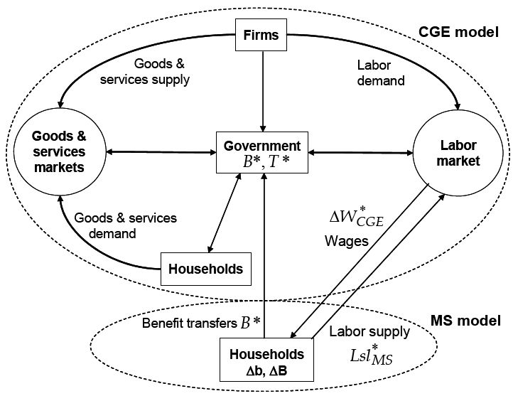
MS–CGE integration.
Tables
Employed and unemployed reweighing for L1 to L5 work factors.
| Facto | Description of the worker | PNAD occupational condition (in 1,000 persons) | Unemployment | CGE model data (in 1,000 persons) | Unemployment rate | Reweighing | |||||
|---|---|---|---|---|---|---|---|---|---|---|---|
| Employed Unemployed Total | Employed Unemployed Total | Employed Unemployed | |||||||||
| L1 | Unskilled informal | 12,890 | 1,567 | 14,457 | 10.8% | 11,714 | 1,418 | 13,132 | 10.8% | 0.9088 | 0.9052 |
| L2 | Skilled informal | 5,694 | 952 | 6,646 | 14.3% | 5,264 | 878 | 6,143 | 14.3% | 0.9245 | 0.9226 |
| L3 | Formal with low skill | 13,923 | 1,349 | 15,272 | 8.8% | 12,274 | 1,184 | 13,458 | 8.8% | 0.8815 | 0.8782 |
| L4 | Formal with average skill | 9,208 | 854 | 10,062 | 8.5% | 8,331 | 774 | 9,105 | 8.5% | 0.9048 | 0.9062 |
| L5 | Formal with ligh skill | 2,211 | 95 | 2,306 | 4.1% | 2,063 | 88 | 2,152 | 4.1% | 0.9334 | 0.9238 |
| TOTALS | 43,926 | 4,817 | 48,734 | 9.9% | 39,647 | 8,537 | 87,788 | 9.7% | |||
-
Source: PNAD 2003, CGE model data base.
Elasticities – Marginal effects for grouping demographics.
| Variable | J + 1 (Men) | J = 2 (Women with children) | J = 3 (Women) | |||
|---|---|---|---|---|---|---|
| Elasticity | S.E. | Elasticity | S.E. | Elasticity | S.E. | |
| Wage elasticity (log w) | −0.0230 | (0.0506) | +0.0328 ** | (0.0070) | +0.1168 ** | (0.0047) |
| Income elasticity (log B) | −0.0009 | (0.0010) | −0.0128 ** | (0.0014) | −0.0082 ** | (0.0008) |
| Income elasticity (log Q) | −0.0026 ** | (0.0002) | −0.0041 ** | (0.0006) | −0.0028 ** | (0.0004) |
-
Note:** significant at 1%; * significant at 5%.
-
Source: Authors’ estimates.
Integration of CGE-MS model for non-labor income (Base 2003).
| Household Income Source | Procedure in the Microsimulation (PNAD 2003) |
|---|---|
| Self Employed Income | CGE results variations of these income sources are applied to the microsimulation model vectors.24 |
| Interest, Dividends and Others and House Rental | CGE results variation of these income flows individualized to the 8 household categories in the model are applied to the microsimulation model vectors.25 |
| Retiree and Pension Public Benefits | The same vector values as in the microsimulation base year model. |
| Retiree and Pension Private Benefits | The same vector values as in the microsimulation base year model. |
| Donation received | The same vector values as in the microsimulation base year model. |
-
Note: For each family, the above sources are deflated by a family specific price index (after simulation).26.
-
Source: Authors’ elaboration.
Total benefits by CGE household category and changes between 2003 and 2005 (R$ thousands).
| 2003 | 2005 | 2005–2003 | ||||
|---|---|---|---|---|---|---|
| Households | Bolsa Família | BPC | Bolsa Família | BPC | Total Increase | Share of Benefits in Total Household Income |
| F1 | 777,344 | 675,171 | 1,829,805 | 1,418,757 | 1,796,048 | 4.31% |
| F2 | 35,269 | 19,741 | 88,412 | 255,354 | 288,755 | 3.01% |
| F3 | 616,145 | 302,187 | 1,250,466 | 410,307 | 742,439 | 5.05% |
| F4 | 810,877 | 2,203,557 | 1,861,258 | 4,346,372 | 3,193,196 | 2.32% |
| F5 | 131,450 | 653,335 | 276,218 | 336,645 | −171,922 | −0.11% |
| F6 | 319,388 | 653,445 | 647,264 | 757,034 | 431,464 | 1.09% |
| F7 | 336,965 | 575,066 | 635,454 | 288,837 | 12,259 | 0.00% |
| F8 | 157,558 | 50,428 | 282,481 | 25,328 | 99,823 | 0.04% |
| Total | 3,185,000 | 5,132,934 | 6,871,361 | 7,838,638 | 6,392,065 | 0.57% |
-
Source: Author’s elaboration based on data from the federal budget and SAM (2003).
Programs’ tax sources in 2005 (R$ thousands).
| Brazil Tax Source | Value | Composition | Equivalent tax in the CGE model |
|---|---|---|---|
| Contribuição para Financiamento da Seguridade Social (COFINS: budget code 153) | 7,570,121 | 51.46% | “COFINS” tax and its value added reform |
| Contribuição Provisória sobre Movimentação Financeira (CPMF: budget code 155) | 5,265,907 | 35.80% | Direct taxes on firms and households |
| Outros Impostos Diretos (Income Tax and other directed taxes) | 993,630 | 6.75% | Direct taxes on firms and households |
| Impostos sobre Produtos (Mix of Indirect Taxes) | 445,959 | 3.03% | Indirect taxes on Revenue |
| Contribuição Social sobre o Lucro das Pessoas Jurídicas (CSLL: budget code 151) | 418,667 | 2.85% | Direct taxes on firms and households |
| Operações de Credito Externas – Em Moeda (budget code 148) | 15,713 | 0.11% | |
| Total | 14,710,000 | 100.00% |
-
Source: Authors’ elaboration.
Macroeconomic indicators (percentage change)*.
| Macroeconomics indicators | SIMU A (%) | SIMU B (%) |
|---|---|---|
| GDP | –0.02 | –0.46 |
| Consumption | 0.50 | –0.35 |
| Investment | –1.42 | –1.04 |
| Public Sector Deficit | +17.87 | +7.38 |
| Exports | (**) | –0.84 |
| Imports | (**) | –1.07 |
| Employment | –0.11 | –0.48 |
| Price Index | 0.13 | 0.65 |
-
Note:
-
(*)
Real percentage change from the CGE base year.
-
(**)
Lower than 0.01%. Source: Authors’ elaboration.
Change in employment from the base-year (%).
| L1 | L2 | L3 | L4 | L5 | L6 | L7 | |
|---|---|---|---|---|---|---|---|
| SIMU A | – 0.13 | – 0.14 | – 0.17 | – 0.06 | – 0.06 | 0,00 | 0,00 |
| SIMU B | – 0.85 | – 0.47 | – 0.47 | – 0.28 | – 0.23 | 0,00 | 0,00 |
-
Note: L1-unskilled informal; L2-skilled informal; L3-low-skilled formal; L4-average-skilled formal; L5- high-skilled formal; L6- low-skilled public servants; L7- high-skilled public servants.
-
Source: Authors’ elaboration.
Change in the average real wage from the base-year (%).
| L1 | L2 | L3 | L4 | L5 | L6 | L7 | |
|---|---|---|---|---|---|---|---|
| SIMU A | + 0,32 | – 0,12 | – 0,04 | – 0,07 | – 0,09 | – 0,04 | – 0,01 |
| SIMU B | – 1,77 | – 0.96 | – 1,52 | – 0,90 | – 1,61 | – 1,66 | – 1,62 |
-
Note: L1-unskilled informal; L2-skilled informal; L3-low-skilled formal; L4-average-skilled formal; L5- high-skilled formal; L6- low-skilled public servants; L7- high-skilled public servants.
-
Source: Authors’ elaboration.
Changes in real payroll from the base-year (%).
| L1 | L2 | L3 | L4 | L5 | L6 | L7 | |
|---|---|---|---|---|---|---|---|
| SIMU A | + 0,19 | – 0,25 | – 0,21 | – 0,13 | – 0,14 | – 0,04 | – 0,01 |
| SIMU B | –2.62 | –1.43 | –1.99 | –1.18 | –1.84 | –1.66 | –1.62 |
-
Note: L1-unskilled informal; L2-skilled informal; L3-low-skilled formal; L4-average-skilled formal; L5- high-skilled formal; L6- low-skilled public servants; L7- high-skilled public servants.
-
Source: Authors’ elaboration.
Differences between first and last SIMU B rounds – selected variables (%).
| wage L1 | wage L2 | wage L3 | wage L4 | wage L5 | pindex | GDP | |
|---|---|---|---|---|---|---|---|
| First round simu B | – 2,16 | – 1,39 | – 1,76 | – 1,29 | – 1,93 | 0.56 | – 0.41 |
| Last round simu B | – 1,77 | – 0.96 | – 1,52 | – 0,90 | – 1,61 | 0,65 | – 0,46 |
-
Source: Authors’ elaboration.
Inequality indicators from household per capita income (base year 2003).
| Inequality Indicators | Base Year | SIMU A | SIMU B | ||
|---|---|---|---|---|---|
| Original | Results** | Change | Results** | Change | |
| Gini Index | 0.5930 | 0.5908 | – 0.37% | 0.5902 | – 0.48% |
| Theil-T Index | 0.7213 | 0.7163 | – 0.69% | 0.7161 | – 0.72% |
-
Source: from the CGE-MS integration model. (base year: 2003 PNAD survey).
Change in household income from the base-year (%).
| Average household income | Original | SIMU A | SIMU B | ||
|---|---|---|---|---|---|
| Values (R$) | Values (R$) | °Change | Values (R$) | Change | |
| National average | 432.36 | 431.59 | −0.18% | 428.84 | −0.81% |
| Household 1 (F1) | 43.88 | 45.89 | 4.58% | 45.76 | 4.28% |
| Household 2 (F2) | 70.20 | 74.90 | 6.70% | 74.89 | 6.69% |
| Household 3 (F3) | 46.87 | 47.89 | 2.17% | 47.78 | 1.94% |
| Household 4 (F4) | 166.42 | 168.19 | 1.06% | 167.67 | 0.75% |
| Household 5 (F5) | 303.65 | 302.57 | –0.36% | 301.23 | –0.80% |
| Household 6 (F6) | 191.94 | 192.31 | 0.19% | 191.76 | –0.09% |
| Household 7 (F7) | 696.64 | 693.84 | –0.40% | 689.33 | –1.05% |
| Household 8 (F8) | 3,015.14 | 2,998.08 | –0.57% | 2,972.50 | –1.41% |
-
Note: F1 – poor urban households headed by active individuals; F2 – poor urban households headed by non-active individuals; F3 – poor rural households; F4 – urban households with low average income; F5 – urban households with medium income; F6 – rural households with medium income; F7 – households with high average income; F8 – households with high income.
-
Source: Authors’ elaboration.
Poverty indicators – PNAD 2003.
| Poverty Indicators | Base year | SIMU A | SIMU B | ||
|---|---|---|---|---|---|
| Results* | Results | Change | Results | Change | |
| Poverty Line (Line = R$ 143,70) | |||||
| P0 | 0.3299 | 0.3256 | –1.29% | 0.3271 | –0.84% |
| P1 | 0.1599 | 0.1579 | –1.26% | 0.1593 | –0.38% |
| P2 | 0.1061 | 0.1047 | –1.28% | 0.1060 | –0.08% |
| Extreme Poverty Lines (Line = R$ 71,84) | |||||
| P0 | 0.1485 | 0.1473 | –0.83% | 0.1485 | 0.01% |
| P1 | 0.0777 | 0.0766 | –1.38% | 0.0778 | 0.18% |
| P2 | 0.0578 | 0.0569 | –1.52% | 0.0580 | 0.40% |
-
Source: Authors’ elaboration.