Public investment in irrigation and training, growth and poverty reduction in Ethiopia
- IESD Research, Ethiopia
- Ethiopian Development Research Institute, Ethiopia
Abstract
This paper analyzes the impacts of public investment in small-scale irrigation and farmer training on growth and agriculture-led development, on food security, and on poverty in Ethiopia. We use a dynamic Computable General Equilibrium (CGE) model linked to a microsimulation model based on the latest household income and expenditure survey, in a top-down approach. All public investments are assumed to increase total factor productivity through increased supply of skilled labor and/or irrigated land. We find that investing in farmer training alone has great potential to increase growth, food security and poverty reduction, given that the economy is labor-intensive. Investing in training combined with irrigation has even greater impacts. An irrigation only approach will not yield the expected results if agricultural labor does not have the required skills. The irrigated agriculture sector has great potential despite its small size. However, for the impact to be notable, important investments are required in the first place to increase the share of irrigated agriculture versus the rain-fed. An agriculture-led development is less likely to occur because: i) of weak forward and backward production linkages between agriculture and manufacturing sectors; ii) a significant share of manufacturing inputs is imported; iii) the resulting contraction in private investment which restrains expansion of the manufacturing and services sectors
1. Introduction
Since 1993, the Government of Ethiopia has implemented an agriculture-led development strategy through its Agricultural Development-led Industrialization (ADLI) policy. Currently, this strategy takes the form of the Growth and Transformation Plan (GTP), a five-year plan which began in the 2010–11 fiscal year. During the implementation of the previous medium-term development strategy, the Plan for Accelerated and Sustained Development to End Poverty (PASDEP) between 2005–06 and 2009–10, Ethiopia’s economic growth averaged 11% per annum. In 2010–11 GDP grew at 11.4 %, slowed down to 8.8% in 2011–12 and picked up to 9.7% in 2012–13.
Recent years have witnessed important declines in Ethiopia’s poverty levels. Poverty measured by real consumption expenditure declined by 14.8% between 1995–96 and 2004–05, reaching 38.7% in 2004–05, and continued to fall to 29.6% in 2010–11 (MOFED 2013). Food poverty also declined from 42% in 1999–00 to 38% in 2004–05 and 33.6% in 2010–11. Poverty remains a rural phenomenon, where over 80% of the population resides. In 2010–11, while the proportion of the population below the poverty line stood at 30.4% in rural areas, it was estimated to be 25.7% in urban settings.
Agriculture plays a significant role in Ethiopia. It contributed up to 50% of GDP on average until 2002–2003. Its share gradually decreased to 46.2 % in 2009–2010 and 41.8% in 2012–2013. However, it still remains the main driver of growth. Moreover, the sector is the economy’s largest employer. A significant proportion (72.6%) of the labor force works in agriculture and related activities. Agriculture also provides the largest source of exports (over 75%), and thus foreign currency inflows, which enable the country to import vital raw materials and inputs, including those essential for agricultural production. Finally, agriculture plays a central role in the production and provision of food. Thus, this sector can strongly contribute to poverty alleviation, as a considerable share of income is spent on food (52%).
At the policy level, agriculture is seen to be a potential source of broader economic growth through its backward and forward production linkages, as well as its consumption linkages with non-agricultural sectors of the economy. Along with education, health, roads, and water, agriculture has been identified by the government as a strategic poverty-oriented sector and has benefited from important public resources and investment. In particular, Ethiopia has allocated on average 10% of its expenditures to agriculture between 2009–10 and 2014–15.
Despite the implementation of ADLI for more than fifteen years, the performance of the agricultural sector remains relatively poor. Productivity gains are to a large extent due to the expansion in cultivated areas and favorable climate with a minimal role for improved technology. Cultivated area, production and productivity have been increasing, but at a decreasing rate (NBE, 2013–14). Peak periods in production and productivity are driven by good climate conditions. Agriculture is mainly rain-fed. Although greater emphasis is being given to irrigation and farmer training in recent years, the share of irrigated area and skilled workers remains small. Only about 9% of arable land was developed under small scale irrigation schemes in 2010–11 (GTP APR 2012–13); i.e. 1,064,200 ha out of a total cultivated area of 11,822,786 ha (Agricultural Sample Survey 2010–11). The share of skilled agricultural labor remains only 17.3%. Vulnerability to climate variability translates into significant fluctuations in agriculture annual GDP growth rates. From as high as 13.5% in 2004–2005, growth rates have subsequently become lower and more varied: 6.2% in 2008–09, 7.6% in 2009–10, 8.9% in 2010–11, 4.9% in 2011–12, and 7.1% in 2012–13.
One of the main reasons for the slower growth of production and productivity of the sector is the shortage of trained manpower in rural areas and very low use of the country’s irrigation potential. In light of this, this paper aims at measuring the potential of investing in irrigation and farmer training. The rest of the paper is organized as follows. Section 2 presents the literature review while Section 3 deals with the modeling framework and data. Section 4 and 5 present the scenarios and results. Section 6 concludes.
2. Literature review
The success story of China’s food self-sufficiency in the 1960s and 1970s, was attributed to a massive investment in irrigation (Huang et al., 2006). Fanadoz (2012) finds that small irrigation schemes (SIS) have greater positive impact on economic growth and poverty reduction in South Africa, but this can be completely missed unless government accompanies SIS revitalization measures with capacity building in basic crop and irrigation management practices, and strengthening institutional and organizational arrangements.
Regarding the economic benefits of education, Croppenstedt et al. (1998) argue that literacy creates awareness and capacity for farmers to adopt modern inputs and improved technologies. Education may enhance farm productivity directly by improving the quality of labor, by increasing the ability to adjust to shocks, and through its effect upon the propensity to successfully adopt innovations. Education is thought to be particularly important to farm production in a rapidly changing technological or economic environment (Shultz 1975). Fan et al (1999) find that in India public spending on rural education has negative and statistically significant effects on rural poverty. Using similar methodology, public expenditure on rural education in China is found to have the largest impact on rural poverty (Fan et al. 2002).
However, when it comes to the impact of general public investment on economic growth we find contrasting results from previous studies. Easterly and Rebelo (1993) find that public investment by central government has a positive and statistically significant effect on economic growth. Devarajan et al. (1996) challenged this finding. When increased public investment in agriculture is financed through cuts elsewhere, it has a negative, and statistically significant, effect on growth.
As it is clearly expressed in the ADLI strategy, agricultural development is expected to stimulate overall economic growth while also reducing poverty and food insecurity. However, there is currently a debate whether Ethiopia should continue with its current agricultural development-led industrialization strategy or make adjustments.
On the one hand, Diao et al. (2007) argue that the emphasis of ADLI and PASDEP on agricultural growth is, in principle, warranted. The results of their paper show that agricultural growth contributes more to overall growth than non-agricultural growth. It also leads to greater poverty reduction by generating proportionately more income for farm households who represent the bulk of the poor. Decomposition of these effects also reveals that consumption linkages are much stronger than production linkages. Early work in India during the Green Revolution indicated that higher-income small farmers spent about half of their incremental farm income on non-farm goods and services as well as another third on perishable agricultural commodities. Thus, consumption linkages from growing farm income can induce sizable indirect effects on rural growth via increased consumer demand for non-agricultural goods and services as well as perishable, high-value farm commodities. On the other hand, the results also clearly show that exclusive focus on agriculture (or insufficient attention to non-agriculture) is counter-productive. Non-agricultural sectors have to grow in order to match the growing supply of agricultural products and increasing demand for non-agricultural products. Otherwise, falling relative prices of agricultural products may dampen the realized gains in growth and poverty reduction.
Furthermore, Mellor and Dorosh (2009) argue that for agriculture to be the driver of the economy, farmers are required to be ‘middle farmers’ and emphasize the need for high levels of government investment. Thus, Ethiopia’s concentration of small-scale farmers presents less capacity to adopt new technologies. Finally, Dercon and Zeitlin (2009) noted that with modest consumption linkages agricultural innovation is not sufficient to drive growth in industry. They find that it may not be necessary for Ethiopian agriculture to be oriented toward the supply of raw materials for industry, nor for all industrial energies to focus on the processing of domestic raw materials. They suggest that the most effective policies to stimulate growth may be those that strengthen domestic and international linkages.
In this context, this paper attempts to empirically test the outcomes and sustainability of ADLI-PASDEP-GTP policy keeping in mind its main objectives: food self-sufficiency, rapid and sustainable growth, and poverty reduction. Our paper contributes to the literature and informs policy design on the outcome of skill development and irrigation investment in Ethiopia and similar countries. It is the first paper to apply a macro-micro approach in analyzing public investment in agriculture in Ethiopia.
3. The modeling framework and data
3.1 The CGE model
The proposed CGE model uses an adapted version of the PEP 1-t model by Decaluwé et al. (2013). A full description of the model can be found in Decaluwé et al. (2013). We will only present here the changes.
3.1.1 The agricultural sector
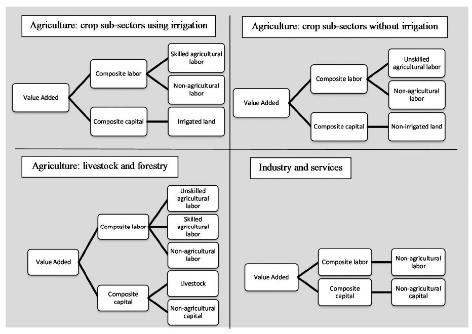
There are 12 agricultural crop sub-sectors1. Each sub-sector is distinguished by whether they use irrigation and skilled agricultural labor. There are 12 sub-sectors utilizing irrigated land, skilled agricultural labor and non-agricultural labor. The other 12 crop sub-sectors combine non-irrigated land, unskilled agricultural labor and non-agricultural labor in their value added (Figure 1).

Nested structure of value added.
The model’s production function is a two-level constant elasticity of substitution (CES) function (Figure 1). In agricultural sectors, at the lowest level, agricultural labor (skilled or unskilled) and non-agricultural labor are aggregated into composite labor. Non-agricultural sectors employ only non-agricultural labor. In parallel, non-agricultural capital, land (irrigated or non-irrigated), and livestock are combined into composite capital. Agricultural sectors do not employ non-agricultural capital except the forestry and fishery sub-sector. Livestock is employed only in the livestock sector. Land is only employed in the 24 agricultural crop sub-sectors. At the intermediate level, composite labor and composite capital are aggregated to form value-added. Finally, value-added is combined in fixed proportions with intermediate inputs to make gross output.
3.1.2 Public investment in training and irrigation
Public investment in training transforms unskilled agricultural labor into skilled agricultural labor. The same applies for land where public investment in irrigation enables the transformation of non-irrigated land into irrigated land.
Total agricultural labor supply, LSTagr, is the sum of skilled LSlagr,qt and unskilled LSlagrnq,t agricultural labor supply. It increases at the fixed population growth rate (Equation 1). Skilled agricultural labor increases with the population growth rate and public investment in training INDcap,training,t (Equation 2). Unskilled agricultural labor supply is endogenously determined as the residue between total agricultural labor and skilled agricultural labor (Equation 3).
σ_training is the elasticity of skilled labor supply to public investment. It is equal to 1. When the investment shock is introduced, it is set at 0.915 so that the average performance between 2009–10 and 2012–13 is obtained.
Public investment in irrigation, INDlandir,j,t increases the amount of irrigated land, KDlandir,j,t at the agricultural sub-sector level by transforming rain-fed land (Equation 5). Total land available for cultivation KSTj,t is the sum of irrigated KDlandir,j,t and non-irrigated land KDlandnir,j,t. It increases at the fixed population growth rate. Non-irrigated land is determined residually (Equation 6) by the difference between total sectoral land supply KSTj,t and irrigated land, KDlandir,t.
where σ_irj is the elasticity of irrigated land supply to public investment. It is equal to 1 except when the investment shock is introduced and it is set to 1.223.
3.1.3 Endogenous household endowments
Our modeling approach assumes that household endowments in labor (trained/skilled and untrained) and in land (irrigated and non-irrigated) are endogenous. Households can modify, through training (or public capital for irrigation), the proportion of skilled/trained and unskilled labor (irrigated and non-irrigated land) they detain. Unskilled agricultural labor and rain-fed land are determined residually for each household. Note that households do not have a demand function for training. We assume that training does not have direct or opportunity costs at the household level.
3.2 Poverty analysis within the CGE framework
The study uses the IFPRI extended standard recursive dynamic CGE modeling system, version 2.00 (Lofgren et al., 2003), for its poverty analysis. This system endogenously estimates the impact of the investment scenarios on poverty by using a “top-down” approach where changes in the CGE model are imported into the microsimulation model. This uses micro data from the 2009–2010 HICES for detailed information on household expenditure. Households are distinguished by income (lower and higher income) and by location (rural, semi urban and urban) in the CGE model. Income and expenditure patterns vary considerably across these household groups. These differences are important for distributional change, since incomes generated by agricultural growth accrue differently to households depending on their location and factor endowments.
In the microsimulation, each of the 27,835 households questioned in survey is linked to the corresponding representative household in the CGE model. A second level of mapping links the commodities in the CGE model and survey with those used in the calculation of the poverty line. Only the latter are considered in the poverty impact analysis. Changes in representative households’ real consumption in the CGE model are then passed down to their corresponding households in the survey. In the next step, real total consumption expenditures are recalculated in the survey. Household size is used to calculate per capita consumption expenditure. Similarly to the representative households in the CGE model, the households in the survey are heterogeneous in their consumption patterns. The micro-simulation model calculates the share of each commodity in total expenditure for each of the survey households. These weights are maintained when post-shock consumption expenditure is calculated. This new level of per capita expenditure is compared to the exogenously given poverty line, and standard poverty measures are recalculated. The Foster Greer and Thorbecke (FGT) poverty measures are applied. The 3781 Birr per year and per adult poverty line used in this study is the official poverty line. In the poverty analysis, consumption is used as the metric to measure poverty.
3.3 Measuring food security within the CGE framework
Availability of, and access to, food are common indicators of food security. Availability of food can be measured by nationwide food supply indicators, while access is captured through household consumption of food staples. Access to food can also be measured through the country’s capacity to finance its current food imports through trade. We focus on the availability approach.
To measure the impact on food insecurity, we use as a proxy the volume of total agricultural food crop production (XSTfood crops,t), the total labor force (Σl LSl,t), and the food price index (CPIfood crops,t). If total agricultural output divided by total labor force increases, this means that there are more goods produced per individual. This is a first indication of the potential for such a policy intervention to increase food availability. However, as our labor force is fixed within a given period of time, the food availability indicator will only reflect changes in the volume of output. To verify whether this type of policy intervention has further potential to contribute to reducing food availability, it is important to look at the changes across time in the food availability index to check whether it allows a more accelerated increase (relative to the first period) in food availability compared to the Business As Usual (BAU) reference scenario. The results may show that the policy has a potential for reducing food insecurity. However, this applies only if consumer prices of food crops remain unchanged or decrease. We upgrade our food availability index (FAindexl) by integrating the consumer price index (Equation 7).
Agricultural output may be destined to export, reducing the food available on the local market. Similarly, food may be imported, increasing food availability. We therefore push our analysis further by using total domestic supply of agricultural products (local output minus exports plus imports). Our second index (FAindex2) uses total food supply (SUPfood crops,t) instead of output (Equation 7). The value of the two indices is equal to 1 in the first period. When it increases, this indicates improvements in food availability.
3.4 Data
The CGE model is calibrated to a social accounting matrix (SAM) of Ethiopia, which was built by the Ethiopian Development Research Institute (EDRI), based on 2005–2006 data. The SAM required adjustments to fit the needs and modeling requirements of the present study. In addition, it has been updated to 2010–2011 to reflect, to the extent possible, the more recent macroeconomic situation and, in particular, the shares of agriculture and crop sub-sectors in GDP. The value of GDP for 2010–2011 at constant market price was used as a reference. Information was taken from National Bank of Ethiopia (NBE) and Ministry of Finance and Economic Development (MOFED) data.
The SAM has 19 production activities of which 14 are agricultural, 3 industrial (industry, agro-processing and manufacturing) and 2 services (private and public). These activities produce 25 commodities (20 agricultural, 3 manufacturing, and 2 services). There are five primary factors of production (agricultural labor, non-agricultural labor, land, livestock, and non-agricultural capital). Agricultural labor and land have been disaggregated using data from the 2010–11 Agriculture Sample Survey. Agricultural labor was disaggregated between skilled and unskilled labor. To disaggregate land between irrigated and non-irrigated land types, the same survey was used. Data show that a very small share of agricultural land is irrigated, although the potential for increases is high. There are six aggregate household groups: rural, small urban and big urban, each disaggregated into lower-income and higher-income categories. The SAM has three tax accounts (direct and indirect taxes and import duty), as well as aggregate accounts for trade margins, government, investment and stock variations, and the rest of the world. Substitution and transformation elasticities have been taken from other studies focusing on the same country (Dorosh & Thurlow 2009).
4. Scenarios
The model is built in such a way that public expenditure in training increases the share of skilled agricultural labor, while investment in irrigation increases the share of irrigated land. We use targets set in the GTP and performances given in the annual GTP progress reports when determining growth in skilled labor and irrigated land as a result of public budget increment. The first three years of the GTP implementation have had the following outcomes (GTP APR 2013–14):
Public expenditure in the agriculture and natural resources increased from 6,998 million ETB in 2009/10 to 14,650 million ETB in 2013/13. This represents an annual average of growth 27.3%.
Land developed under small scale irrigation schemes benefiting small holder farmers increased from 853,000 ha in 2009/10 to 1,830,000 ha in 2012/13 with an annual average growth of 28.6%.
The number of farmers benefiting from agricultural extension services rose from 5.1 million farmers and pastoralists in 2009/10 to 11.6 million having increased by a yearly average of 32.2%.
Crop productivity (quintal per hectare) increased from 15.4 in 2009/10 to 17.8 in 2012/13. The average crop productivity growth over these four years reaching 3.9%.
Based on this, a 10% increase in the training budget is assumed to enable an 11.8% increment in skilled agricultural labor, while a 10% increase in irrigation spending enables a 10.5% growth of irrigated land supply. To determine the productivity impact of public investment in agriculture, we look at studies that focused on public investment in agriculture and irrigation in other African countries. Benin et al. (2009) find that a 1% increase in public spending on agriculture is associated with a 0.15% increase in agricultural labor productivity in Ghana. Diao et al. (2010) find that a 1% increase in agricultural spending is associated with a 0.24% annual increase in agricultural TFP in Nigeria. Thurlow et al. (2007) use an elasticity of TFP of 0.20 for investment in irrigation and 0.15 for spending on extension services in Kenya. Other studies utilize agricultural growth instead of agricultural TFP as the dependent variable when measuring the impact of public investment in agriculture2.
The productivity shocks we implement are based on elasticity of TFP to public investment following Thurlow et al. (2007). Table 1 summarizes the three scenarios implemented in this paper.
Summary of scenarios.
| Scenarios | Time frame | |
|---|---|---|
| Simulation 1 | 10% increase in public investment for farmer training | 2nd period |
| 11.8% increase in skilled agricultural labor supply | 3rd period | |
| 1.5% improvement in TFP in irrigated agriculture crop sectors | 3rd period | |
| Simulation 2 | 10% increase in public investment in irrigation uniformly across all agricultural sub-sectors | 2nd period |
| 10.5% increase in irrigated land | 3rd period | |
| 2% improvement in TFP in irrigated agriculture crop sectors | 3rd period | |
| Simulation 3 | Simulation 1 + Simulation 2 for public investment | 2nd period |
| 3.5% improvement in TFP in irrigated agriculture crop sectors | 3rd period |
5. Simulation results
The analysis of the three simulations is to be considered within the following context. The disaggregation of agricultural land in the SAM reflects the situation in 2010–11 when a mere 8.8% of total cultivated area was developed under irrigation schemes. Likewise, the share of skilled agricultural labor is low, reaching 17.3% in 2010–11. Overall when irrigated land and skilled agricultural labor are combined to form what we qualify as ‘irrigated’ agriculture, its share in total real GDP in the SAM is very small (4.6%) while its share in total agricultural GDP is 10.3%. Because of its small size, the 11.8% increase in skilled agricultural labor increases the share of skilled farmers to 19.3% of total agricultural workers, thereby increasing the share of irrigated agriculture sectors to 12% of agricultural real GDP and 5.4% of total real GDP. Similarly, the 10.5% increase in irrigated land increases the share of irrigated land to 9.7% of total land, thus increasing the share of irrigated agriculture to 10.7% of agricultural GDP (4.8% of total GDP). When the two investments are combined, the share of irrigated agriculture reaches 12.4% of agricultural GDP and 5.6% of total GDP.
Reporting of results focuses on two indicative years: 2014–15, which is the timeline for attaining the targets set in the GTP, and 2019–20, which represents the end of the 2010–2020 Agricultural Sector Policy and Investment Framework (PIF). The Business As Usual (BAU) or reference scenario is the basis for comparison, without the new investments. Changes in 2014–15 and 2019–20 are reported relative to the BAU levels in the corresponding years and on a cumulative basis when specified. The presentation of the policy simulation results are structured to address the three main objectives of this paper:
Potential for growth and an agriculture-led development
Potential for reducing food insecurity
Potential for poverty reduction
5.1 Impact on agricultural growth and overall GDP: Is there an agriculture-led development?
The increased pool of skilled labor and/or irrigated land, together with the increase in TFP associated with the higher number of skilled labor and/or irrigated land, has a small but positive impact on GDP. As presented in Table 2, total agricultural GDP increases in all three scenarios, although more when public spending combines irrigation and training, followed by investment in irrigation alone. Agricultural GDP is driven by the expansion of the irrigated agricultural sector. Although rain-fed agriculture contracts, the net impact on agriculture is positive. GDP in the manufacturing sector declines a little (because of a crowding-out effect), while it increases slightly in services sector. In addition, public investment in training has a crowding-out effect across all scenarios (Table 2). The reduction in private investment affects the growth potential of the economy, in particular the manufacturing (and service) sectors, which are highly capital-intensive.
Macroeconomic results (% change from reference scenario).
| Investment in training | Investment in irrigation | Investment in irrigation + training | |||||
|---|---|---|---|---|---|---|---|
| 2014–15 | 2019–20 | 2014–15 | 2019–20 | 2014–15 | 2019–20 | ||
| GDP | Agriculture | 0.16 | 0.16 | 0.21 | 0.21 | 0.41 | 0.41 |
| Irrigated agriculture | 16.63 | 16.62 | 3.91 | 3.90 | 20.91 | 20.89 | |
| Rain-fed agriculture | −2.78 | −2.79 | −0.43 | −0.43 | −3.22 | −3.24 | |
| Manufacturing | −0.17 | −0.48 | −0.03 | −0.06 | −0.21 | −0.55 | |
| Services | 0.03 | 0.03 | −0.01 | −0.03 | 0.02 | 0.00 | |
| TOTAL | 0.07 | 0.04 | 0.09 | 0.07 | 0.17 | 0.13 | |
| Investment | Private | −1.95 | −2.26 | −0.17 | −0.20 | −2.13 | −2.46 |
| Public | 3.69 | 3.69 | 0.32 | 0.32 | 4.01 | 4.01 | |
| TOTAL | −0.03 | −0.07 | 0.01 | 0.00 | −0.02 | −0.06 | |
| Agriculture | −0.37 | −0.44 | −0.28 | −0.29 | −0.71 | −0.79 | |
| Consumer | Agricultural food crops | −0.62 | −0.70 | −0.32 | −0.32 | −0.99 | −1.07 |
| Price | Manufacturing | 0.13 | 0.19 | −0.02 | −0.01 | 0.09 | 0.17 |
| Index | Services | 0.21 | 0.50 | 0.07 | 0.09 | 0.29 | 0.60 |
| TOTAL | −0.08 | −0.03 | −0.12 | −0.11 | −0.23 | −0.17 | |
| Exports | Agriculture | 0.30 | 0.42 | 0.79 | 0.31 | 0.42 | 0.79 |
| Industry | −0.23 | −0.01 | −0.23 | −0.50 | −0.04 | −0.54 | |
| Services | −0.28 | −0.05 | −0.34 | −0.68 | −0.09 | −0.77 | |
| TOTAL | −0.08 | 0.11 | 0.05 | −0.33 | 0.09 | −0.22 | |
| Imports | Agriculture | −0.46 | −0.10 | −0.58 | −0.60 | −0.11 | −0.73 |
| Industry | −0.06 | 0.00 | −0.07 | −0.18 | −0.01 | −0.19 | |
| Services | 0.20 | 0.09 | 0.30 | 0.41 | 0.11 | 0.53 | |
| TOTAL | −0.03 | 0.01 | −0.02 | −0.09 | 0.01 | −0.08 | |
| Output | Agriculture | 0.17 | 0.17 | 0.21 | 0.21 | 0.42 | 0.42 |
| Irrigated agriculture | 16.98 | 16.96 | 3.68 | 3.68 | 21.01 | 20.99 | |
| Rain-fed agriculture | −2.82 | −2.84 | −0.38 | −0.39 | −3.22 | −3.24 | |
| Manufacturing | −0.18 | −0.48 | −0.03 | −0.06 | −0.21 | −0.55 | |
| Services | 0.02 | 0.02 | −0.01 | −0.03 | 0.01 | −0.01 | |
| TOTAL | 0.03 | −0.03 | 0.07 | 0.05 | 0.11 | 0.03 | |
To assess the potential of public investment to generate agriculture-led development, we look at production and consumption linkages. Agriculture is linked to other sectors through forward and backward linkages. Backward linkages imply an increase in demand for industrial products used as inputs for agricultural production. Public investment in training and/or irrigation results in a slight increase in agricultural output (Table 2). Although agriculture is not intensive in intermediate inputs, it uses 51.8% of agricultural products, 46.3% of manufacturing inputs (essentially consisting of fertilizers and chemicals) and 1.9% of services (mainly financial and transport services). Agriculture-led development through backward linkages does not generate growth in the manufacturing and service sectors, where output contracts or remains nearly unchanged.
The three investments scenarios reduce the agricultural intermediate demand price index. This may be a source of agriculture-led development. Industries that are intensive in agricultural intermediate inputs, in particular agro-processing industries, are likely to benefit from the fall in the prices of agricultural products.
Agriculture-led development can also occur via consumption linkages. Increases in agricultural income could lead to increased demand for non-agricultural final consumption goods. However, this depends on the composition and income elasticity of household consumption. Changes in agricultural factor income are presented in Table 3.
Changes in agricultural factors income in real terms ((% change from reference scenario).
| Investment in training | Investment in irrigation | Investment in irrigation + training | ||||
|---|---|---|---|---|---|---|
| 2014–15 | 2019–20 | 2014–15 | 2019–20 | 2014–15 | 2019–20 | |
| Skilled agricultural labor | 11.78 | 11.59 | −8.67 | −8.51 | 11.72 | 11.53 |
| Unskilled agricultural labor | −2.00 | −2.16 | 1.60 | 1.75 | −2.03 | −2.19 |
| Total agricultural labor | 0.38 | 0.22 | −0.38 | −0.22 | 0.39 | 0.23 |
| Irrigated land | 8.80 | 8.58 | 1.11 | 1.06 | 8.28 | 8.06 |
| Non-irrigated land | −3.49 | −3.68 | 2.78 | 2.98 | −3.57 | −3.76 |
| Livestock | 0.00 | −0.06 | 0.12 | 0.17 | 0.03 | −0.02 |
| Total agricultural capital | −1.51 | −1.65 | 1.67 | 1.79 | −1.50 | −1.64 |
| Total agricultural factors | −0.05 | −0.23 | 0.08 | 0.25 | −0.04 | −0.22 |
Total agricultural labor income declines in the second scenario, driven by the drop in skilled agricultural wages, while it increases slightly when investment is geared towards training and training combined with irrigation. Similarly, land income declines in the first and second scenarios, as a result of the drop in returns to rain-fed land, which overrides the important increase in returns to irrigated land. Overall, total agricultural factor income declines slightly except in the irrigation investment scenario. Consumption linkages are not likely to be strong in this context.
Changes in agricultural output and prices affect the country’s competitiveness. Agriculture plays an important role in Ethiopia as of the main source of exports, where export revenue to finance the import of essential raw material and inputs.
Agricultural exports increase across the three scenarios, although only slightly. Exports increase significantly in export-intensive irrigated agricultural sectors (Table A1 in Annex). Exports of non-agricultural products decline a little, as output has contracted or did not increase enough while prices have increased. Total imports fall in the first and last scenarios and remain unchanged in the second one. Imports of agricultural products decline in all scenarios, as locally produced commodities are relatively cheaper. Imports of manufacturing goods remain unchanged or decline slightly across all scenarios. Imported services increase slightly, essentially driven by demand for trade services by the agricultural sector for exporting purposes
5.2 Impact on food security
As presented earlier, food security is affected by agricultural output and commodity prices. As presented in the above section, agricultural output only slightly increased. In parallel, the consumer price index has declined, driven by agricultural and food crop prices (Table 2). Figure 2 presents the changes in the food availability indexes. Both indexes show that the policy has potential for increasing food availability.
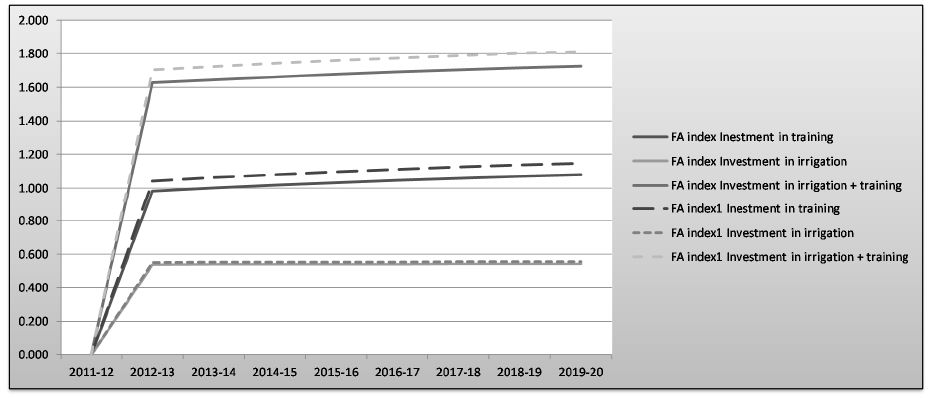
Changes in food availability index: FAindex and FAindex1 (% change from reference scenario).
Whether we use output or supply of food crops, all investment schemes have potential to reduce food insecurity (Figure 2). Combining training and irrigation investment, which yields higher productivity, is more likely to increase food availability. Investing in farmer training has significantly more potential to increasing food availability than investing in irrigation only.
Finally, agricultural output in food crops may be destined for export, reducing the food available on the local market. Similarly, food may be imported, increasing food availability. When comparing the results from the two food availability indexes, we find that these investments have a higher impact on food security measured by the total supply of food crops, as opposed to total output of food crops.
5.3 Impact on poverty
The micro-simulation results show that poverty declines across all investment scenarios (Table 4). The poverty gain is small but positive. Gains are higher when investment targets irrigation and training simultaneously. Investing in training is more likely to generate more poverty reduction than investments in training. Furthermore, when looking at rural areas, where most of the poor are concentrated, rural poverty declines systematically more than urban poverty in the first and third scenarios. In the second scenario, urban poverty declines more than rural poverty. This is because the higher income rural households are much more endowed with land, implying that higher land income benefits the non-poor.
Changes in FGT indices (% change from reference scenario).
| 2014–15 | 2019–20 | |||||
|---|---|---|---|---|---|---|
| Investment in training | Investment in irrigation | Investment in irrigation + training | Investment in training | Investment in irrigation | Investment in irrigation + training | |
| Poverty incidence | ||||||
| National | −0.47 | −0.06 | −0.75 | −0.20 | −0.06 | −0.46 |
| Rural | −0.51 | −0.05 | −0.82 | −0.22 | 0.00 | −0.46 |
| Urban | −0.20 | −0.14 | −0.38 | −0.07 | −0.41 | −0.43 |
| Poverty gap | ||||||
| National | −0.58 | −0.15 | −0.78 | −0.27 | −0.14 | −0.46 |
| Rural | −0.63 | −0.10 | −0.77 | −0.30 | −0.08 | −0.43 |
| Urban | −0.28 | −0.44 | −0.82 | −0.04 | −0.51 | −0.65 |
| Poverty severity | ||||||
| National | −0.63 | −0.16 | −0.84 | −0.28 | −0.14 | −0.48 |
| Rural | −0.68 | −0.10 | −0.82 | −0.32 | −0.08 | −0.44 |
| Urban | −0.34 | −0.52 | −0.96 | −0.05 | −0.56 | −0.72 |
Poverty depth and poverty severity also decline nationally in all three investment schemes. However, at a more disaggregate level, the policy intervention is not pro-poor. The poverty gap is much higher for the rural population, but it declines less than for the urban population, except in the first scenario. Looking at the poverty severity index, rural households have a higher risk of being in poverty than urban households, but their poverty is not significantly more severe (2.0 for rural and 1.8 for urban). Nevertheless, the policy is not pro-poor, as the poverty severity index declines much more for urban households. However, poverty incidence, poverty gap and poverty severity decline for all types of households. In addition, rural settings comprise over 80% of the population.
When we compare poverty reduction with the reference scenario in 2010–11, we find that by 2014–15, investing both in irrigation and training is likely to reduce poverty by an extra 2.4% compared to 1.5% if investment targets training alone and 0.2% if investment targets irrigation only (Table 5). The poverty reduction gains are lower in 2019–20 and investment in irrigation tends to reduce urban poverty significantly more than rural poverty.
Changes in poverty incidence: national rural and urban (cumulative % change from reference scenario in 2010–11).
| 2014–15 | 2019–20 | |||||
|---|---|---|---|---|---|---|
| Investment in training | Investment in irrigation | Investment in irrigation + training | Investment in training | Investment in irrigation | Investment in irrigation + training | |
| National | −1.50 | −0.21 | −2.42 | −0.24 | −0.07 | −0.55 |
| Rural | −1.50 | −0.21 | −2.42 | −0.24 | −0.07 | −0.55 |
| Urban | −0.67 | −0.46 | −1.25 | −0.08 | −0.50 | −0.52 |
Investing in training and irrigation simultaneously yields the best poverty reduction outcome, lifting 900 thousand Ethiopians out of poverty. Investing in farmer training plays a bigger role than investing in irrigation.
Changes in the number of poor (cumulative % change from reference scenario in 2010–11).
| BAU reference scenario | Investment in training | Investment in irrigation | Investment in irrigation + training | |
|---|---|---|---|---|
| Total number of poor 2014/15 | −3,477,899.67 | −3,566,496 | −3,490,060 | −3,620,623 |
| Total number of poor 2019/20 | −7,058,304.39 | −7,089,129 | −7,067,681 | −7,128,995 |
| Total number of poor since policy implementation | −654,067 | −185,948 | −900,702 |
6. Conclusion
This paper simulates the potential impact of public investment in farmer training and irrigation schemes, two priority areas of the Ethiopian government’s agriculture development policy.
We find that investing in farmer training alone has great potential for growth, food security and poverty reduction. When combined with investment in irrigation, it has even greater potential. However, investing in irrigation alone will not yield the expected results without simultaneously ensuring that agricultural labor has the required training. Despite its small size, the irrigated agriculture sector has great potential. However, for the impact to be important and enhance agriculture-led industrialization, substantial investments may be required to increase the share of irrigated versus rain-fed agriculture. Greater effort and commitment is therefore needed for irrigated agriculture to reach a significant size before production linkages are able to enhance growth in manufacturing sectors.
Our analysis shows that the Ethiopian government’s policy strategy regarding agriculture development has great potential for reducing poverty and food insecurity. However, agriculture-led development does not occur in our case also because public investment has crowding-out effects that hinder the expansion of the manufacturing and service sectors. Financing such investment plans may require an alternative allocation of public resources or even a different financing mechanism.
Our analytical framework does not account for private costs, which can be particularly high when setting up irrigation schemes. As Ethiopian rural farmers are generally poor, availability of credit will be essential to the success of such investments. Training these farmers will be indispensable if investment in irrigation is to be productive. Put this way, it is essential to combine investment in irrigation with skill development. From a cost perspective, and given the current structure of Ethiopia’s agricultural system, investing in skill development may have a strong impact in a relatively shorter period of time.
Footnotes
1.
These are teff, barley, wheat, maize, sorghum, pulses, vegetables & fruit, oil seeds, cash crops, enset, cereal grains and other crops, and coffee.
2.
Estimates of the elasticity of agricultural growth to public investment in the literature are discussed in Mitik and Engida (2012).
References
-
1
Public expenditures and agricultural productivity in Ghana. Contributed PaperIAAE, Beijing.
-
2
Assessing the impact of the National Agricultural Advisory Services (NAADS) in the Uganda rural livelihoods. Discussion Paper 00724Washington, D.C.: International Food Policy Research Institute.
-
3
Irrigation impacts on income inequality and poverty alleviation: policy issues and options for improved management of irrigation systems. Working Paper No. 39International Water Management Institute.
-
4
Agricultural Sample Survey 2009/10 to 2014/15Agricultural Sample Survey 2009/10 to 2014/15.
-
5
Report on the 2013 National Labour Force SurveyReport on the 2013 National Labour Force Survey.
-
6
Technology adoption in the presence of constraints: The case of fertiliser demand in Ethiopiamimeo, Oxford: Centre for the Study of African Economies.
-
7
The PEP Standard General Equilibrum Model Single-Country, Recursive Dynamic Version PEP-1-tPoverty and Economic Policy (PEP) Research Network.
-
8
‘Rethinking Agriculture and Growth in Ethiopia: A Conceptual Discussion’Paper prepared as part of a study on Agriculture and growth in Ethiopia, a project funded by Department for International Development (DFID).
-
9
‘Growth from Agriculture in Ethiopia: Indentifying Key Constraints’Paper prepared as part of a study on Agriculture and growth in Ethiopia, a project funded by Department for International Development (DFID).
-
10
‘The Composition of Public Expenditure and Economic Growth’Journal of Monetary Economics 37:313–344.
-
11
Agricultural Growth Linkages in Ethiopia: Estimates using Fixed and Flexible Price Models. Discussion Paper No. 00695Washington, D.C.: International Food Policy Research Institute.
-
12
‘Growth options and poverty reduction in Ethiopia – An economy-wide model analysis’Food Policy 32:205–228.
-
13
‘Agricultural Growth and Investment Options for Poverty Reduction in Nigeria’. Discussion Paper 00954Washington, D.C.: International Food Policy Research Institute.
-
14
‘Implications of Accelerated Agricultural Growth on Household Incomes and Poverty in Ethiopia: A General Equilibrium Analysis’. ESSP2 Discussion Paper No. 002‘Implications of Accelerated Agricultural Growth on Household Incomes and Poverty in Ethiopia: A General Equilibrium Analysis’. ESSP2 Discussion Paper No. 002.
-
15
‘Fiscal Policy and Economic Growth: An Empirical Investigation’Journal of Monetary Economics 32:417–458.
-
16
Linkages Between Government Spending, Growth and Poverty in Rural India. Research Report 110Washington, DC: International Food Policy Research Institute.
-
17
‘Government spending, growth and poverty: an analysis of interlinkages in rural India’. Environment and Production Technology Division Discussion Paper No. 33‘Government spending, growth and poverty: an analysis of interlinkages in rural India’. Environment and Production Technology Division Discussion Paper No. 33.
-
18
Growth, Inequality and Poverty in Rural China: The Role of Public Investments. Research Report 125Washington, DC: International Food Policy Research Institute.
-
19
‘Public expenditure, growth and poverty reduction in rural Uganda’. DSGD Discussion paper No. 4‘Public expenditure, growth and poverty reduction in rural Uganda’. DSGD Discussion paper No. 4.
-
20
‘Revitalization of smallholder irrigation schemes for poverty alleviation and household food security in South Africa: A review’African Journal of Agricultural Research 7:1956–1969.
- 21
-
22
‘Irrigation, Agricultural Performance and Poverty Reduction in China’Food Policy 31:30–52.
-
23
‘Poverty and Inequality Analysis in a General Equilibrium Framework: The Representative Household Approach’In: F Bourguignon, LA Pereira da Silva, editors. The Impact of Economic Policies on Poverty and Income Distribution: Evaluation Techniques and Tools. Washington, D.C. and New York: World Bank and Oxford University Press. pp. 325–337.
-
24
Agriculture and the Economic Transformation of Ethiopia. ESSP-II Discussion Paper 12International Food Policy Research Institute, Addis Ababa.
-
25
Growth and Transformation Plan 2010/11-2014/15Growth and Transformation Plan 2010/11-2014/15, Volume 1: Main Text, Addis Ababa, November.
-
26
Federal Democratic Republic of Ethiopia Growth and Transformation Plan Annual Progress Report for F.Y. 2010/11Federal Democratic Republic of Ethiopia Growth and Transformation Plan Annual Progress Report for F.Y. 2010/11.
- 27
-
28
Federal Democratic Republic of Ethiopia Growth and Transformation Plan Annual Progress Report for F.Y. 2011/12Federal Democratic Republic of Ethiopia Growth and Transformation Plan Annual Progress Report for F.Y. 2011/12.
-
29
Federal Democratic Republic of Ethiopia Growth and Transformation Plan Annual Progress Report for F.Y. 2012/13Federal Democratic Republic of Ethiopia Growth and Transformation Plan Annual Progress Report for F.Y. 2012/13.
-
30
Public investment in irrigation and training for an agriculture-led development: a CGE approach for Ethiopia. Working Paper 2013-02Partnership for Economic Policy.
- 31
-
32
‘The value of ability to deal with disequilibria’Journal of Economic Literature 13:827–896.
-
33
Rural Investments to Accelerate Growth and Poverty Reduction in Kenya. Discussion Paper 00723International Food Policy Research Institute.
Article and author information
Author details
Acknowledgements
Acknowledgment: This work was carried out with financial and scientific support from the Partnership for Economic Policy (PEP), with funding from the Department for International Development (DFID) of the United Kingdom (or UK Aid), and the Government of Canada through the International Development Research Center (IDRC). We are grateful to Bernard Decaluwé, Hélène Maisonnave and André Lemelin for their invaluable comments and suggestions. The authors alone are responsible for all errors and omissions.
Publication history
- Version of Record published: April 30, 2016 (version 1)
Copyright
© 2016, Beyene and Engida
This article is distributed under the terms of the Creative Commons Attribution License, which permits unrestricted use and redistribution provided that the original author and source are credited.