A microsimulation model for risk in Irish tillage farming
- Rural Economy and Development Programme, Ireland
Abstract
Tillage farmers must manage numerous economic risks including uncertain yields and prices. Despite the presence of government payments, these factors can generate a relatively high variability in farm income. The improved management of farm income variability can contribute towards stability in household consumption, support for farm investments, further investment in child education and a reduction in the mental stress associated with variable incomes. In this paper, we develop a new farm-level stochastic microsimulation model to simulate the degree of risk attached to the production of Ireland’s main tillage grain crop i.e. spring barley for animal feed usage. Forward contracting is the main available risk management tool for Irish tillage farmers. Our microsimulation model is extended in order to estimate the impact of forward contracting on farm income risk. Our results show that forward contracting can reduce farm income risk significantly but that other stable sources of income are probably necessary to contain the exposure to the income risk attached to cereal production. The model is capable of addressing the income risk associated with multiple crops although this version of the model is confined to one particular crop. The model can be further extended to accommodate other risk management tools such as crop insurance or a farm management deposit scheme. This will allow policymakers, farmers and other interested parties to assess the impact of alternative risk management policies on the heterogeneous pool of Irish tillage farmers.
1. Introduction
Microsimulation models are increasingly being applied to research topics in agricultural economics (Shrestha et al. 2007; Hynes et al. 2009; Ramilan et al. 2011 and O’Donoghue 2013). Microsimulation models have much in common with traditional farm simulation models as both are frequently used to simulate policy and economic change although the biological component of farm level models makes them somewhat distinct (Richardson et al. 2014). In this paper, we introduce a stochastic farm-level microsimulation model with the objective of estimating the degree of income risk associated with tillage production on Irish farms. The model is extended further to examine the direct impact of forward selling a fixed proportion of cereal output on the variability of profit margins. This is the first attempt in the microsimulation literature to analyse the contribution of forward contracts or other financial risk management tools towards the containment of risk in agriculture.
Tillage farms in Ireland are an interesting case study as these farms face a number of serious challenges and risks which could potentially threaten their economic viability and survival into the future. These include a heavy dependence on direct payments (Hennessy et al. 2008), competition for access to land from the more profitable dairy sector (Läpple & Hennessy 2012) and risks associated with nutrient loss and the wider environment (Buckley & Carney 2013). Despite the presence of government payments, the risks associated with uncertain yields (production risk) and prices for individual crops (market risk) can be sufficient to generate unusually high income variability. Numerous studies have examined the role of these two variables in influencing income variability (e.g. Coble et al. 2002; Goodwin and Ker 2002).
The high exposure to production and market related income variability is particularly relevant for those farms with relatively low government payments and without stable off-farm income (Jetté-Nantel et al. 2011). There is a clear absence of empirical analysis regarding the economic impact of income risk and risk management tools for the main grain crops in Irish agriculture. Numerous studies have provided stochastic analysis of the risk associated with uncertain yields and prices in other areas of Irish agriculture e.g. Shalloo et al. (2004), Finneran et al. (2011) and Clancy et al. (2012) but none of these deal with the main grain crops. We develop a stochastic microsimulation model for the risk associated with uncertain prices and yields in the production of Spring Barley, the most commonly produced crop on Irish tillage farms (Holden et al. 2003; Kennedy and Connery 2005).
The development of the stochastic Microsimulation model largely follows the semi-parametric Monte Carlo simulation techniques outlined in Richardson et al. (2000) and Richardson et al. (2014) and adopted elsewhere by Archer and Reicosky (2009), Wilson and Dahl (2011) and Feng et al. (2014) among others. In our case, the microsimulation model is based on actual farms in the panel component of the Teagasc National Farm Survey. Kimura and Le Thi (2011, p6) explain that accounting for farm level characteristics is a critical part of risk analysis and point out that “using the cross-section data or aggregated time series data does not properly measure the producer’s exposure to risks”.
In recent years, the microsimulation literature has addressed risk-related topics such as poverty (Navicke et al. 2014) and financial market volatility (Lux and Marchesi 2000) but microsimulation techniques are less frequently applied to risk-related issues within agriculture. The capacity of microsimulation modelling to deal with farm heterogeneity can be of immense added value particularly in the area of risk where risk attitude and the exposure to risk can vary substantially across farms.
In the next section, we describe the recent evolution of risk management policies and tools relevant to Irish tillage farmers and indeed tillage farmers across the European Union. We follow this with a description of the data utilised to develop the model. In Section 4, we discuss the methodology used to develop the stochastic model. In Section 5, we discuss some results relating to the riskiness of profit margins in the production of spring barley and the potential impact of forward contracting on risk. This is followed finally by the conclusion.
2. Risk management: tools and government policies
Policies in relation to risk in Irish agriculture have largely been determined at an EU level since Ireland entered the European Community in 1973. On Ireland’s entry into the community at the same time as Britain, the policy of intervention prices placed a floor on the degree of downside risk faced by farmers in both Ireland and Britain. For Irish farmers, the intervention prices determined a large share of total government payments until the MacSharry reforms and the introduction of direct payments in 1992/1993 (Hennessy et al. 2014). Sckokai and Moro (2009) explain that the MacSharry reforms were only partially decoupled from production given their connection with “decisions through the land allocation mechanism”. This contrasts with the subsequent 2003 reforms and the introduction of the fully decoupled Single Farm Payment in 2005 in Ireland, although a number of Member States opted to retain some coupled payments.
The rapid decline in the intervention prices in the 1990s and early 2000s in conjunction with significantly reduced export subsidies introduced a much greater exposure to output price risk. At the same time, the introduction of direct payments helped to offset some of this risk although this varied across farms. Research has identified changes in risk attitude as a result of these policy reforms (Koundouri et al. 2009). Our microsimulation excludes this kind of behavioural component so that we do not address the potential effect that these policy changes may have had on risk attitude.
During the latest CAP reform package for 2014–2020, the real decline in the overall budget for direct payments is being accompanied by the emergence of an income stabilisation tool (IST) (European Commission, 2011) although the degree to which this tool has been implemented varies across Member States. In the EC proposal, the new tool should provide compensation to farmers who experience a severe drop in their income. Support can only be granted “where the drop of income exceeds 30% of the average annual income of the individual farmer in the preceding three-year period or a three-year average based on the preceding five year period excluding the highest and lowest entry. Furthermore, “payments by the mutual fund to farmers shall compensate for not more than 70% of the income lost” (European Commission 2011).
A few studies have sought to estimate the economic outcomes that this tool can produce. Mary et al. (2014) have estimated that farm income volatility in France declines by more than 35 per cent with the introduction of the IST but may generate output distortions. Finger and El Benni (2014a) find that the IST mechanism significantly reduces income inequality among Swiss farms. Finger and El Benni (2014b) conclude that the specification of the farm-level reference income should account for observed income trends as “the average-based approaches cause lower than expected indemnification levels for farmers with increasing incomes, and higher indemnifications if farm incomes are decreasing over time.”
The empirical analysis in this paper does not focus on the potential economic impact of these non-established tools and instead concentrates on the direct impacts from an existing risk management tool namely the forward contracting tool. Seifert et al. (2004) define a forward contract simply as “an agreement to buy a commodity at a certain future time for a certain price”. Microsimulation models have rarely incorporated the contribution of financial risk management tools such as forward contracts and futures towards the management of income variability in commodity or other financial markets.
In our farm-based example, the commodity in question is spring barley for animal feed usage. We seek to identify the direct impact on the riskiness of farm profit of entering into a forward contract at different prices and under a range of alternative yield and price scenarios. Tillage farmers in Ireland have access to a very limited number of risk management tools to manage risk with forward contracting being the main available market risk management tool. Hennessy et al. (2014) have estimated that approximately 30 per cent of Irish tillage farms availed of the forward contracting tool during 2012.
The limited availability of risk management tools in Ireland contrasts with the situation in the United States where Pennings et al. (2008) report that a majority of U.S. crop producers employ more than one risk management tool. Forward contracts, basis contracts, futures contracts, catastrophic coverage and crop revenue coverage appear to be the most commonly adopted tools. In Australia, the Farm Management deposit (FMD) scheme has been widely adopted as a form of risk management tool with the total number of accounts reaching almost 46,000 in June 2014 and total deposits peaking at over $4bn (Australian Government, 2014).
This scheme allows ‘eligible primary producers’ to deposit pre-tax income in years of high income, which can be accessed subsequently in years of low income. The income in the FMD account is tax deductible in the financial year the deposit is made and becomes taxable in the financial year of the withdrawl. From July 2016, the cap on deposits rises from AUD ($) 400,000 to AUD ($) 800,000 (Australian Government, 2016).
The widespread use of risk management tools in the United States has generated a significant literature examining the economic impact of tool adoption at the farm level. Cornaggia (2013) finds that risk management leads to greater productivity by relaxing financial constraints suggesting that producers that hedge are more likely to receive access to finance, which can then be used ‘to finance productivity-enhancing investments’. Glauber (2013) concludes that crop revenue insurance coverage based on expected prices compares favourably to fixed-price supports such as countercyclical payments and marketing assistance loans. Goodwin and Smith (2013) argue however, that the burdens associated with the collection of tax revenues to fund the subsidized crop insurance program can generate a large number of distortions both within agriculture and the aggregate economy.
It is envisaged that the future development of this farm-level microsimulation model will allow us to make some worthwhile judgements on the potential effectiveness of the above policies on risk and profitability in Irish tillage farming and the potential effectiveness of alternative risk management tools which may include forward contracting. The wider effects on the non-agricultural economy are however, probably beyond the scope of the model.
3. Data
In this section, we describe the data source used to construct the farm-level model. This data includes the Teagasc National Farm Survey, the CSO Data on crop yields, FAO data on international crop yields and a crop price database collected and maintained by the Agricultural Economics and Farm Survey department of Teagasc Rural Economy. The objectives of the National Farm Survey (NFS) are to
Determine the financial situation on Irish farms by measuring the level of gross output, costs, income, investment and indebtedness across the spectrum of farming systems and sizes,
Provide data on Irish farm incomes to the EU Commission in Brussels (FADN),
Measure the current levels of, and variation in, farm performance for use as standards for farm management purposes, and
Provide a database for economic and rural development research and policy analysis.
To achieve these objectives, a farm accounts book is recorded for each year on a random sample of farms, selected by the CSO, throughout the country. For this analysis, the Teagasc NFS micro data spans the period from 2004 to 2013. The panel is unbalanced in the sense that there is some attrition from year to year as farmers leave the sample and are replaced by other farms. The attrition rate is relatively low however and new farmers are introduced during the period to maintain a representative sample that is usually kept to between 900 and 1100 farms.
For our purposes, we concentrate on specialist and non-specialist tillage farmers who produce spring barley for animal feed usage. We concentrate on this subset of farmers as spring barley is the most common grain crop produced by Irish farmers. We have excluded malted spring barley due to the price differential between malted barley and barley for animal feed usage. We have excluded some growers of spring barley (animal feed use) for a number of reasons. First, it is critical that each farm in the analysis has a sufficient number of historical yields for the generation of stochastic projections. As in the case of the Italian analysis by Kimura and Le Thi (2011), we include all crop producers that have remained in the sample for at least five years between 2004 and 2013.
There are a total of 138 farms meeting the above criteria and these farms are therefore considered to be ‘the selected sample’ and are available for the stochastic analysis. This includes some specialist tillage farms which are largely focused on cereal production and non-specialist cereal producers, who engage primarily in livestock and/or milk production and for whom cereal production is a secondary activity. There is some attrition in our data in that only 37 farms have historical data for Spring Barley in all of the ten relevant years. The 138 farms represent approximately 8,700 Spring Barley growers. Our sample is therefore representative of the vast majority of spring barley growers in the country. The Census of Agriculture 2010 showed that there were 9,058 spring barley growers (inc. malted barley) in Ireland during that year (CSO, 2012). Our sample includes farms that rotate crops from time to time. This explains the relatively high number of growers being represented.
In Table 1, we display some summary statistics to compare our selected sample of tillage farmers with all other tillage farms in the Teagasc National Farm Survey. This will allow us to examine the representativeness of the selected sample. The statistics are weighted according to the weights provided in the Teagasc National Farm Survey micro-data. The comparison distinguishes between those with no record of producing spring barley for animal feed, those farms with a record of less than five years in producing this crop and those farms comprising the selected sample i.e. those farms with at least five years of production in spring barley for animal feed usage. Some farmers concentrate their activities on other grain crops and are therefore excluded from this initial version of the model. It is intended that the model will eventually broaden to incorporate other grain crops when the sample size becomes sufficient.
Statistics for the selected sample and other tillage producers.
| Other Tillage Producers | The selected sample | ||
|---|---|---|---|
| No Spring Barley | Less than Five Years of Spring Barley | Five Years Plus of Spring Barley | |
| Spring Barley Yield [Animal Feed] | N/A | 5.69 | 6.04 |
| Average Spring Barley [Animal Feed] Hectares | 0.00 | 6.54 | 10.45 |
| Average Malted Spring Barley Hectares | 5.69 | 1.37 | 0.34 |
| Farm Size [Number of Hectares | 59.23 | 54.03 | 69.71 |
| Land Owned | 51.97 | 44.44 | 59.25 |
| Land Rented In | 11.02 | 14.45 | 15.01 |
| Total Pasture Hectares | 30.43 | 30.63 | 38.50 |
| Total Tillage Hectares | 24.28 | 20.36 | 27.97 |
| Number of Crops in Each Year | 1.11 | 1.38 | 1.59 |
| Mainly Tillage (0,1) | 0.37 | 0.47 | 0.51 |
| Specialist Dairy (0,1) | 0.20 | 0.13 | 0.06 |
| Livestock Units | 59.48 | 56.80 | 69.73 |
| Livestock Units Per Hectare | 1.07 | 1.01 | 0.97 |
| Farm Operator Age | 50.99 | 51.90 | 55.98 |
| Mean Farm Income | 38,353 | 31,140 | 36,750 |
| Mean Market Farm Income | 19,790 | 15,446 | 11,780 |
| Mean Single Farm Payment | 17,482 | 14,722 | 23,991 |
| Off-Farm Employment Operator | 0.34 | 0.38 | 0.24 |
| Off-Farm Employment Spouse | 0.23 | 0.31 | 0.28 |
| Sample size | 49 | 240 | 138 |
-
Source: Authors Calculations using Teagasc National Farm Survey Data 2005–2013.
Table 1 shows that the selected sample tends to achieve a higher yield per hectare than those farms with less than five observations perhaps reflecting the better performance and growing conditions for farms in the selected sample. It may be the case that some farmers respond to poor yield outcomes by ceasing the production of spring barley and we should consider this in any assessment of the model results. For the selected sample, the average number of hectares of spring barley production appears quite low at approximately 10.45 hectares. This is due to the fact that some of these farms will have recorded years without production of spring barley for animal feed. A substantial proportion of activity on many of these farms is allocated to livestock production. For instance, among the selected sample, an average of approximately 38.5 hectares is devoted to livestock production. This exceeds the average number of hectares allocated to tillage production. A relatively small proportion (~ six per cent) of the selected sample is engaged in specialist dairy farming. This contrasts with 20 per cent for those crop-producers with no spring barley for animal feed usage.
In terms of farm income, it appears that the selected sample has higher farm income than those farms with fewer observations of spring barley. This is mainly driven by differences in the size of the single farm payment as opposed to market-based activities. The average size of the single farm payment is quite substantial and capable of providing a role as a risk management tool and perhaps crowd out the demand for the forward contracting tool and other financial risk management tools. The average age of the farm operator is also higher among the selected sample which may have some effect on risk management decision-making. The differences in sample characteristics mean that we should be careful in interpreting the results. The eventual results will apply to those farms with a relatively high number of years with spring barley production and may not be so relevant for those farms with an occasional production of this crop.
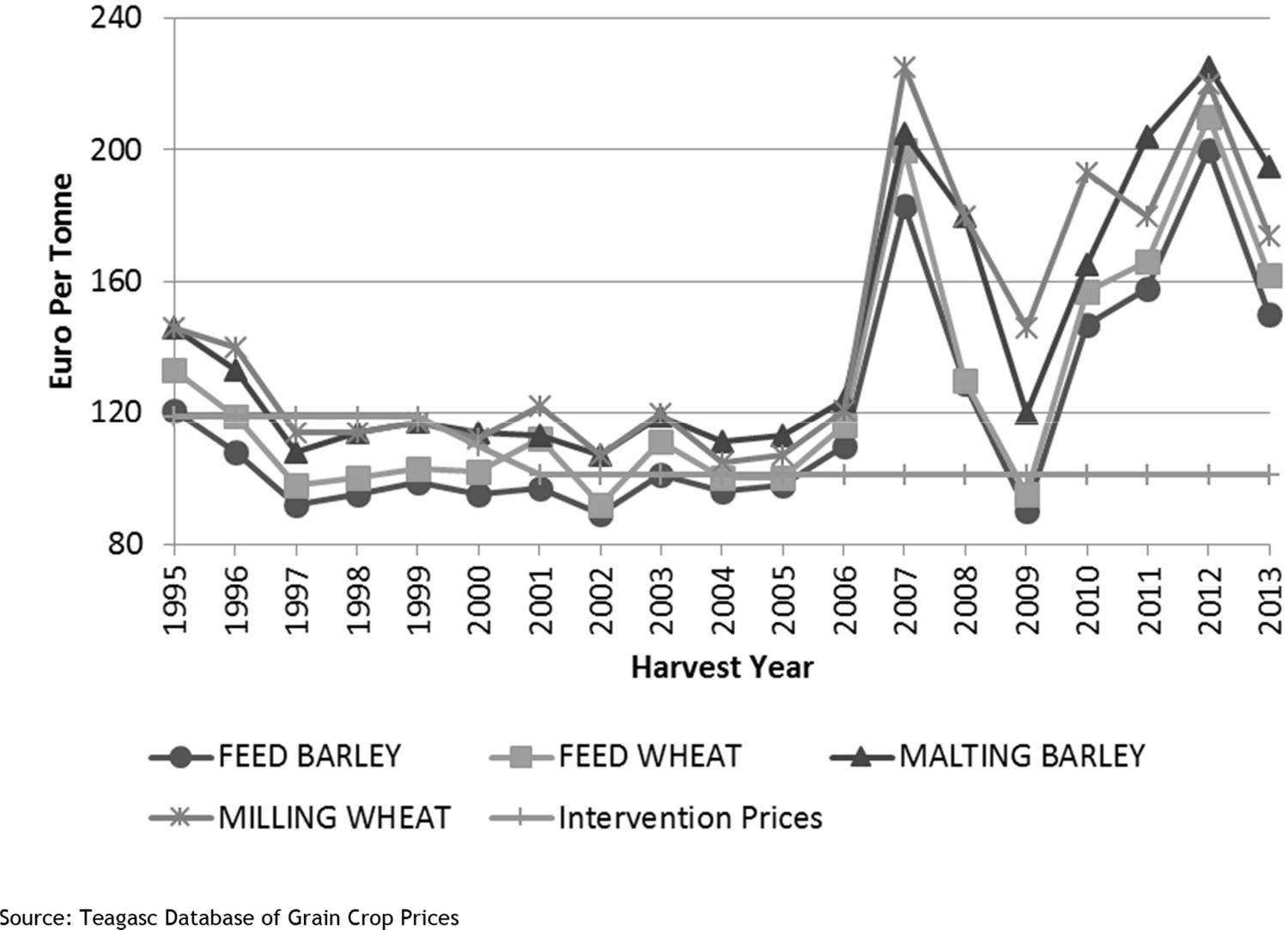
As in the case of dairy farmers, the volatility in output and input prices has increased in the past decade. This is part of a wider global trend which has received much attention in the academic literature (see for example Abbott et al. 2011). In Figure 1, we present the recent output price trends for the main grain crops including Barley for animal feed usage. Historically, there have been significant differences in price between Malted Barley and Barley for animal feed use with Malted Barley commanding the higher output price. Despite this price differential, the Barley for animal feed use is more commonly grown in Ireland. The size of the livestock sector in Ireland demands a large supply of grain crops for animal feed use.
Historical price trends for selected grain crops (€).
One can see from Figure 1 that the price for Feed Barley has lagged behind Malted Barley for the entire period. The price for Feed Barley has closely followed that for Feed Wheat especially since the year 2000. Perhaps, the most striking aspect of this graph is the apparent increase in the volatility of these output prices since 2006. Both Feed Barley and Feed Wheat prices hit the intervention price in the demand slump of 2009 having reached record nominal prices in 2007. It does appear however, that the intervention price is becoming less significant over time. During the 1990s and early 2000s, the market price for Barley was frequently below the intervention price. Grant (2010) explains that this greatly reduced the risks faced by producers and “led to the appearance of the famous butter mountains, wine lakes etc.” Policy has responded by phasing out the option of intervention, reducing the intervention price to near world market levels or alternatively abolishing the option of intervention for particular commodities.
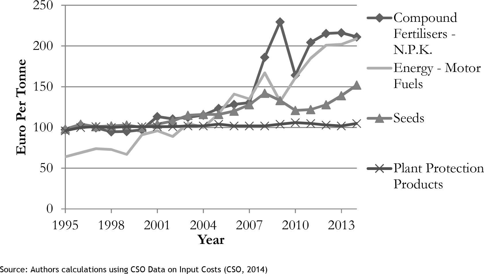
The profitability of Barley production is dependent on both the output price and the relevant input prices. In terms of input prices, the price of Fertilizer, Machinery Hire, Crop Protection and Seeds are particularly important. In Figure 2, we display the cost price indices for these four inputs. We use the index for motor fuel as a substitute for machinery hire.

Cost indices for key inputs at sowing time (Index 2000)1.
The model includes information on international crop yields and domestic crop prices given that international crop yields can influence domestic crop prices. A correlation matrix of these variables is generated which we discuss in more detail in the next section. The correlations between crop yields are made at the aggregate level using data taken from the CSO rather than farm level data from the Teagasc National Farm Survey. This is a necessary step given that the vast majority of the farms in the sample do not produce all of the relevant crops in the same year i.e. Barley, Wheat and Oats. We are therefore assuming that the correlations between the yields of Barley, Wheat and Oats, as calculated using the CSO aggregate statistics are appropriate for the variety of farms in our sample.
4. The model
Our model provides an estimate of Market Gross Margin for the production of Spring Barley (animal feed use) for each farm under 500 alternative output price and yield scenarios, generated using the SIMETAR software package. We therefore account for the risk associated with these two random variables. The stochastic returns are based on market gross margin rather than market net margin. The market gross margin excludes the deduction of farm overheads such as depreciation, interest repayments and other expenditure items such as electricity, light and heat costs which cannot easily be attributed to a particular farming activity. The market net margin is the profit measure which includes the deduction of these overhead items. In this section, we describe the steps required to estimate the stochastic market gross margin beginning with a formal definition of the market gross margin. This is followed by an explanation of the steps required to deliver stochastic estimates for each of the components in the model.
The formula for the market gross margin function is the following:
p output price per unit of Spring Barley
q yield per hectare of Spring Barley crop
HA Land Size in Number of Hectares cultivated of Spring Barley. It is assumed that the total number of hectares is unchanged from the most recently available data year.2
DC Direct Costs including Hired Machinery, Seeds, Crop Protection, Fertiliser, Transport Costs, Labour and Other Direct Costs. The Direct Costs are crop specific.
Stochastic prices
The stochastic output prices p are estimated based on the historical information on output prices from the Teagasc database, a series of ordinary least squares (OLS) regressions and the Teagasc Outlook deterministic projections for 2014. These projections were carried out in December 2013 and therefore prior to the sowing of crops for the 2014 harvest. At this time, the Teagasc outlook indicated a deterministic projection of approximately 160 euro per tonne for Winter Wheat. The outlook did not explicitly provide a deterministic estimate for Spring Barley prices. However, the Spring Barley price typically follows the trend in Winter Wheat prices albeit at a slightly lower level. For 2014, this would have suggested a deterministic projection in the region of 150 to 160 euro per tonne (Thorne 2013). The regression based model should ideally provide a deterministic value in this region for 2014.
The regression based model would be unnecessary if futures prices on spring barley for animal feed usage were widely available in all historical years. In the presence of future prices, one could simply assume that the futures price at any given time represents the best available guide to the predicted price for the crop at harvest time. In contrast to malted barley, there are limited futures markets for spring barley for animal feed usage although such markets do exist in Australia and Hungary. In the United Kingdom, there does exist a LIFFE feed wheat futures market and this can often prove to be a useful guide to the future feed barley price given the expected high correlation between both feed wheat and feed barley prices. The Agriculture and Horticulture Development Board (AHDB) provides a frequently updated information source on developments in these markets (AHDB 2016).
Given the absence of a suitable feed barley futures market, we therefore rely on the OLS regression approach outlined in (Richardson et al. 2000).
In estimating a stochastic model for spring barley prices, a number of important decisions must be made including the choice of probability distribution. Richardson et al. (2000) advise that ten observations per farm provides a sample size that is too small for the use of standardized probability distributions such as the weibull distribution or beta distribution. We therefore employ an empirical distribution. Richardson et al. (2000) conclude that an empirical distribution “avoids enforcing a specific distribution on the variables and does not limit the ability of the model to deal with correlation and heteroscedasticity”.
As proposed by Richardson et al. (2000), the first step in estimating the parameters for a multivariate empirical (MVE) distribution is to separate the random and non-random components for each of the stochastic variables. We utilise an ordinary least squares (OLS) regression to separate the random and non-random components and therefore identify whether or not a deterministic component appears to have historically existed for Spring Barley prices.
This longitudinal regression is carried out with the historical data on Spring Barley output prices covering the period from 1995 to 2013. The relevant period involved changes such as a sharp increase in economic growth among lower and middle income countries and a sharp rise in livestock feed use in developing countries, both factors placing upward pressure on cereal prices. During this time, the share of land required to be allocated to setaside was reduced to zero, which ought to have placed some downward pressure on prices3. Incorporating all of these factors into an econometric model would add a great degree of complexity with little added value.
The harvest year is the only independent variable in this model and is represented by Trendt. In this case, the notation c represents the particular crop (in this case spring barley). The objective is simply to identify whether or not a time trend has existed during this time. This econometric model could be made much more complex by attempts to incorporate various national and global supply and demand factors as determinants of the predicted price in each given year. We argue however, that this would introduce a great degree of complexity without much added value. In the absence of a time trend, it can be assumed that the simple mean () represents the predicted value of the Output price in each year as given in Equation 3.
In this regression-based approach, the residuals are a useful proxy for the degree to which the output price deviates from the expected. The residuals or random component (e) is calculated by subtracting the predicted or non-random component of the variable from the observed value in each year.
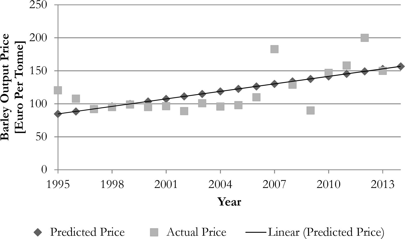
One can see from Figure 3, the linear predicted trend in output price and the actual outcome price in each year with the difference representing the residual or random component. CV represents the coefficient of variation for the recent history of spring barley prices. The value of 20.45 per cent corresponds very closely to the findings of Nayak and Turvey (2000) for a sample of farmers in Ontario, Canada.
Actual and linear predicted spring barley price (€) 1995–2013.
Figure 3 shows that in most years, the actual output price has not deviated substantially from the linear predicted price but there are exceptions including 2007 when a boom in commodities prices occurred and 2012 when drought in major crop producing countries affected global supply. The onset of the severe global recession in 2009 manifested itself in unusually low output prices for grain crops.
The next step is to convert the residuals êct into fractional deviates about their respective deterministic components.
For instance, where the predicted output price is 160 per tonne, a residual or deviation of 16 euro per tonne represents a fractional deviate of ten per cent i.e. . The historical range of fractional deviates can therefore be used to estimate the degree of risk attached to output prices in the near future. This is, of course, based on the assumption that the historical distribution of unexpected price changes is an appropriate guide to the stochastic distribution of prices in the future.
The relative deviates Dct are then sorted from the minimum deviate to the maximum deviate. N denotes the total number of recorded observations in the sample, in this case 19, each representing one year of historical price data. Prior to this sorting exercise, the creation of pseudo minimums and pseudo maximums are necessary for each random yield and price variable. This ensures that the simulated distribution returns the extreme values. As in the case of Richardson et al. (2000), the pseudo-minimum and maximums are defined to be very close to the observed minimum and maximum.
The upper and lower bound for the deviates Dcn are estimated in the following:
The addition of these upper and lower bounds means that there are 21 initial points for the empirical distribution of output prices i.e. 19 historical observations plus the lower and upper bounds.
The fractional deviates are then sorted and probabilities are assigned to each of the sorted deviates in the following
Based on this sorting exercise, we can produce Table 2 showing the historical fractional deviates sorted from lowest to highest and the probability attached to each outcome. At this stage, the deterministic price will be established using either Eq. 2 or Eq. 3. In the case of the Spring Barley price, a deterministic component does appear to exist. The significant time trend (Eq. 2) provides an annual gradual price increase of 3.80 euro per tonne.
In Table 2, one can see that the minimum fractional deviate is approximately -0.364. This implies that the lowest estimated output price for the simulated year will be no lower than 36.4 per cent below the deterministic price of 156.736 euro per tonne. Table 2 also shows that the maximum fractional deviate is approximately 0.445. This implies that the maximum estimated output price for the simulated year will be no higher than 44.5 per cent above the deterministic price.
Parameters for an empirical distribution of feed barley price in 2014.
| Historical Ranking | Deterministic Component | Sorted Fractional Deviates Dct | Cumulative Probability (F(Dc) |
|---|---|---|---|
| Min | 156.736 | −0.364135974 | 0 |
| 1 | 156.736 | −0.346796166 | 0.0263 |
| 2 | 156.736 | −0.200781935 | 0.0789 |
| 3 | 156.736 | −0.19998511 | 0.1316 |
| 4 | 156.736 | −0.19211783 | 0.1842 |
| 5 | 156.736 | −0.12981906 | 0.2368 |
| 6 | 156.736 | −0.12203359 | 0.2895 |
| 7 | 156.736 | −0.10178267 | 0.3421 |
| 8 | 156.736 | −0.08118956 | 0.3947 |
| 9 | 156.736 | −0.03725432 | 0.4474 |
| 10 | 156.736 | −0.01925512 | 0.5 |
| 11 | 156.736 | −0.00869402 | 0.5526 |
| 12 | 156.736 | −0.00817022 | 0.6053 |
| 13 | 156.736 | −0.002380722 | 0.6579 |
| 14 | 156.736 | 0.038333195 | 0.7105 |
| 15 | 156.736 | 0.086928907 | 0.7632 |
| 16 | 156.736 | 0.219717674 | 0.8158 |
| 17 | 156.736 | 0.34089299 | 0.8684 |
| 18 | 156.736 | 0.405517738 | 0.9211 |
| 19 | 156.736 | 0.424213082 | 0.9737 |
| Max | 156.736 | 0.445423736 | 1 |
These 21 alternative fractional deviates and the deterministic predicted output price (Eq. 2) are subsequently used to estimate 500 alternative price and yield scenarios for each of the 138 farms in the sample but a number of other steps must be first carried out. The next stage is to describe the steps required to estimate the parameters for the stochastic distribution of crop yields, which are an additional source of production risk for tillage producers.
Stochastic yields
In contrast to the output prices, the stochastic yields are estimated for each farm in the data. This is carried out in order to reflect the wide disparities in average yield and the variability of yields between farms. The variability of within-farm crop yields far exceeds the within-farm variability in crop output prices. The estimation of stochastic yields is a formidable exercise given that there are 138 farms in our sample. In addition, the stochastic yields are estimated at a national level in line with the Eqs. 2–12. These national level estimates are less critical for the model but they do allow for the construction of a correlation matrix of international yields and prices, which can be used in the future to simulate the impact of movements in international crop yields on domestic Irish crop prices.
As in the case of the output price, a series of OLS regressions are applied. In this case, the regression is repeated for each farm in the sample in order to reflect differences between the farms in both average crop yield and its variability. The notation i represents each individual farm in the dataset. For international crop yields, we simply exclude the notation i as those regressions are based on national level data.
The Harvest year is again the only independent variable in this model. The objective is simply to identify whether or not a time trend has existed during this time. On some farms, the coefficient on the time trend will be insignificant. In the absence of a time trend, it can be assumed that the historical mean of yields () represents the predicted value of the Yield YDiCt in each year as given in Equation 14.
As in the case of prices, the residuals or random component (ê) is calculated by subtracting the predicted or non-random component of the variable from the observed value in each year.
In a small minority of cases, the linear trend in the crop yield will be unrealistically high or low and we therefore place an upper and lower bound on the beta coefficient for the trend in crop yields i.e. we do not allow the beta coefficient to exceed 0.25 or reach below −0.25. This essentially imposes a limit of approximately minus four or plus four per cent on the deterministic crop yield. We have chosen this threshold on the basis that the average crop yield growth tends to be in the region of one per cent per annum in Ireland. In some cases, a coefficient limit in excess of 0.25 would suggest that crop yields are changing at approximately five per cent per annum which far exceeds the national average of approximately plus one per cent.
As in the case of the output prices, the fractional deviates for each historical crop yield are estimated, in this case at the farm level. For farms with ten years of historical data, there will be twelve alternative fractional deviates. This includes the ten historical deviates and a pseudo maximum and pseudo minimum estimate. The large number of alternative farm-level estimates means that the deviates cannot be summarised in one table.
Given the possible historical relationship between international crop yields and domestic Irish crop yields and prices, there is a case for including the international crop yield deviates in our model. Irish crop production forms a small share of global production and international crop yields can be a significant driver of variability in Irish crop prices. In our model, we include yields for Irish Spring Barley, Irish Oats, Irish Wheat, UK Barley, UK Wheat, UK Rye, UK Oats and USA Soybeans. Our initial model included a larger range of crop yields from French, German and USA agriculture but these were excluded due to the absence of a significant correlation between these crop yields and Irish crop prices or yields.
As in the case of Richardson et al. (2000), we develop an intra-temporal correlation matrix to account for these potential international relationships. The intra-temporal correlation matrix is calculated using the unsorted, random components (eit) from equation 3 and is demonstrated in Richardson (2000) for a 2 X 2 matrix. Many of these correlations are not entirely critical to the income risk results displayed later in the paper but they can be used to develop the model in the future.
In Table 4 of the Appendix, we provide the correlation matrix. The results show that crop yields in Ireland are highly correlated at a national level. For instance, the correlation coefficient between Barley and Oats Yields is 0.72 and 0.84 between Barley and Wheat. As expected, Irish crop yields are much less correlated with international crop yields although there does appear to be a relatively high correlation between UK and Irish Wheat yields. USA Soybean yields are included in this model due to the significant relationship between USA Soybean yields and Irish Malted Barley prices and the coefficients are relatively high for other Irish crop prices.
Irish crop prices are also highly correlated with one another. For instance, Irish feed barley prices and Irish feed wheat prices have a correlation coefficient 0.97. This suggests that the production of multiple crops, in a given year, may have a limited role as a form of risk management. A weak positive correlation coefficient is found between the yield and price for spring barley (animal feed use). The weak correlation is unsurprising given that domestic crop yields are unlikely to be a major driver of Irish crop prices. The positive sign of the coefficient should not be overly surprising given that the literature has sometimes found that expected crop prices can influence the final yield at harvest time (Miao et al. (2015).
Simulation
A number of further steps must be carried out in order to generate the simulations. The correlation matrix is transformed in SIMETAR into a 14x1 correlated uniform standard deviates (CUSD) matrix in line with Richardson (2008, p.28). This matrix retains the correlation coefficients provided in appendix Table 4. An empirical distribution is then simulated in SIMETAR using the EMP() function. The function assumes a continuous distribution so it interpolates between the 21 specified points on the distribution. This interpolation exercise generates Correlated Fractional Deviates CFDi(14x1).
These deviates contain information on the size of the deviates for each variable and the correlation between the domestic and international price and yield variables. These Correlated Fractional Deviates are applied to the predicted price and yield values to provide us with an initial simulated value for the yield or price in the simulation year.
where represents initial simulated value for the price or yield variable and represents the deterministic predicted value for each of these variables as estimated in Eq. 2–3 and Eq. 13–14.
The Simulate Command in SIMETAR then produces the entire 500 simulated scenarios for both output price and yield. The generation of 500 alternative output price and yield scenarios means that we can produce 500 alternative Gross Output per Hectare scenarios given that Gross Output per hectare is the product of total price p multiplied by yield per hectare q as shown in the following:
Direct costs
For the estimation of Total Market Gross Margin, it is necessary to deduct the direct costs of production from output as given in Eq. 1. In the case of Direct Costs, we have made some assumptions to simplify the procedure. The cost of each direct cost item is assumed to be given at the time of sowing. It is assumed that the price of the fertiliser, crop protection and other direct costs are known by the farmer at this point in time and that no risk is attached to fluctuations in the price of direct costs.
The direct costs for each farm are based on historical farm-level direct costs per hectare for each individual cost item listed above and CSO price data for the first three months of the projection year, in this case 2014. We assume however, that there is no behavioural response to changes in fertiliser prices or other direct costs from the historical data to the projection year. This may impact on the overall results given that some farms only have historical data for the 2004–2009 period and therefore prior to the large increase in motor fuel costs. We therefore test the sensitivity of our results by excluding those farms with less than eight years of data. This is found to have little impact on the overall results and these results are available on request.
Quality acceptance
Due to data limitations, this research does not explicitly model the risk attached to the quality acceptance. Wilson and Dahl (2011) is one of the few examples to have explicitly modelled this source of risk, with their study concentrating on the case of Durum Wheat production in the USA. The risk of the barley being rejected by potential buyers on the basis of poor quality is a risk that is very relevant for both producers of barley for malting purposes and barley for animal feed usage. For instance, a farmer may intend to grow barley for sale as malting barley but it may be rejected by potential buyers and the farmer will therefore resort to selling the barley as animal feed or alternatively using the barley to feed their own livestock. Our data suggests that the vast majority of malting barley producers have at some point classified a proportion of their barley production as barley for animal feed usage although it is not clear if this is a result of quality issues or something more deliberate.4
The degree of risk attached to quality acceptance differs somewhat between producers of malting barley and barley for animal feed usage. Quality acceptance is a risk for malting barley growers given the demanding standards for malting barley and the price differential between malting barley and barley for animal feed usage. However, these producers do have the option of selling the product as animal feed. For producers of spring barley for animal feed usage, the alternatives are much less rewarding as a failure to meet quality standards is likely to imply a zero payoff. On the other hand, the standards associated with quality acceptance for barley for animal feed usage are lower than for malting barley and ceteris paribus the likelihood of rejection is likely to be lower as a result.
Forward contracts
Forward contracting is the main available risk management tool for Irish tillage farmers. We estimate the impact of forward contracting on farm income risk and the direct impact of this tool on farm income. The degree of income risk is based on the stochastic projection of the Market Gross Margin. We calculate the degree of income variability σgross under three situations 1) where no forward contracts or other financial risk management tool are adopted 2) where 20 per cent of expected production is forward sold at 150 euro per tonne and 3) where 35 per cent of expected production is forward sold at 150 euro per tonne. Given that forward contracting reduces the likelihood of the farmer receiving very low output prices, one may expect that forward contracting will reduce the degree of income variability. Our results will show the degree to which the income variability changes in response to the adoption of the forward contract.
In addition to the risk-reducing benefits of forward contracting, there are usually accounting costs associated with the adoption of the tool. The Grain merchant only has the incentive to offer a forward contract at less than or close to the expected market price. At the same time, a risk averse farmer will, by definition, be willing to enter into a forward contract at a level somewhat below the market expected price. We therefore show the profit impact of forward contract adoption under a situation where the farmer enters into a contract at 150 euro per tonne and therefore slightly below the expected price of 157 euro per tonne. We find that this will on average lead to a fall in income for the average income tillage farmer.5
5. Results
In this section, we present the simulation results showing the degree of income variability attached to the production of spring barley for animal feed usage and the degree to which the forward contracting risk management tool can reduce this income variability and therefore contribute towards managing income risk. We begin this section with the stochastic projections for the output price as this is the main contributor to income risk. This is followed by the results with respect to the riskiness of crop yield and the results relating to the riskiness of the market gross margin.
Risk and price
In Figure 4, we show the entire simulated distribution for the output price. One can see that the probability of a price greater than 150 euro per tonne is estimated to be slightly greater than 50 per cent in our simulation year, in this case 2014. The average simulated price in SIMETAR is 157 euro per tonne. There is estimated to be only a ten per cent chance of the price falling below 120 euro per tonne. At the other end of the distribution, there is an estimated ten per cent chance of the price exceeding 215 euro per tonne.
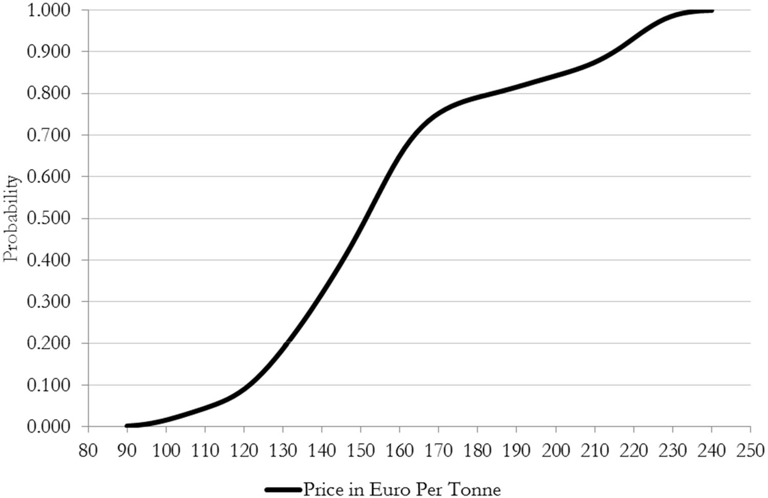
Cumulative distribution function of the feed barley price in 2014.
Risk and yield
In Figure 5, we plot the cumulative distribution of farms according to the simulated coefficient of variation in crop yields. On the y-axis lies the cumulative distribution with the value one representing the entire 138 farms. This provides some indication about the differences between farms in crop yield variability. One can see from Figure 5 that the coefficient of variation is approximately 12 to 14 per cent for the median farm i.e. the 69th highest value for income variability in the sample. This suggests that the variability in crop yields tends to be lower than the variability in output prices, a finding similar to (Nayak & Turvey 2000) but we should exercise some caution in the interpretation given that the yields are given at the individual farm level while the crop prices are aggregate indicators. Kimura and LeThi (2011) explain that aggregated data can underestimate the risk for a particular variable. There are a minority of cases where the simulated crop yield variability is in excess of twenty per cent. In these cases, the simulated degree of variability in crop yields is likely to exceed the output price variability. Conversely, there are a significant minority of farms (~15 per cent) with relatively low crop yield variability of less than eight per cent.
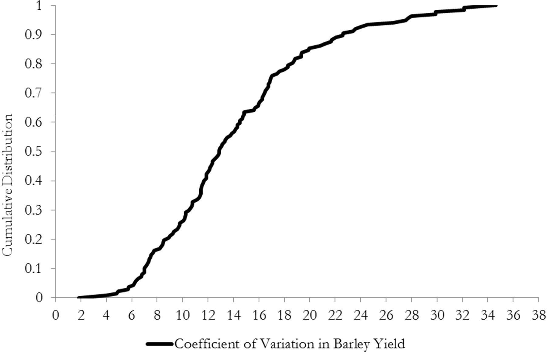
Cumulative distribution of the variability in barley yield in 2014.
Risk and market gross margin
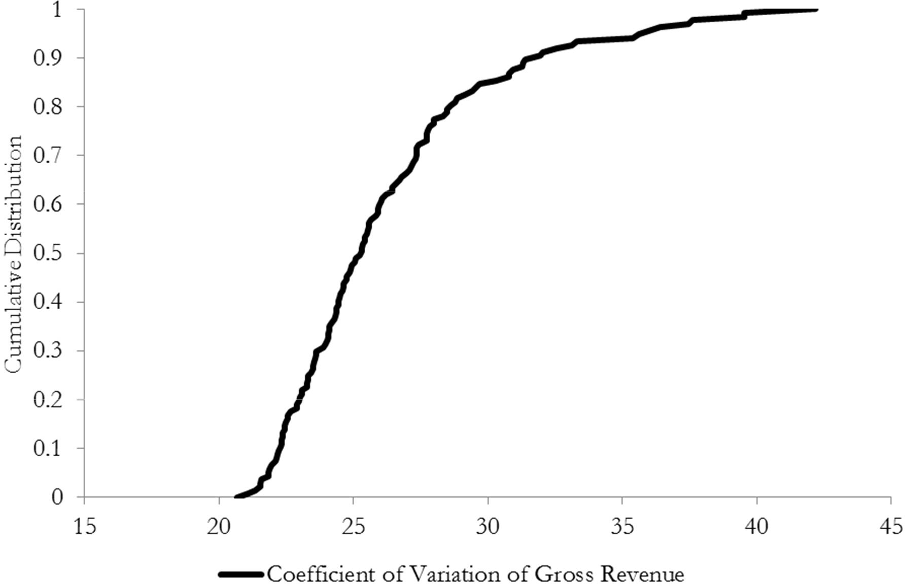
The low correlation between Irish domestic crop yields and crop prices is important in determining the variability of market-based gross revenue and market-based gross margin. In many large crop producing regions or countries, the domestic crop yield or growing conditions have a significantly negative relationship with crop prices in a given year (Hennessy et al. 1997; Hudson & Coble 1999 and Goodwin & Schnepf 2000). This helps suppress the degree of downside revenue risk, as situations of both low output price and low yield become less probable. The absence of a significantly negative relationship in the Irish case means that Irish tillage farmers, ceteris paribus, may face more risk than would be the case in a large crop producing country such as the United States or the Ukraine.
The absence of a significant trade-off between domestic crop yields and prices means that the market revenues tend to be much more variable than either the output crop price or crop yield alone.
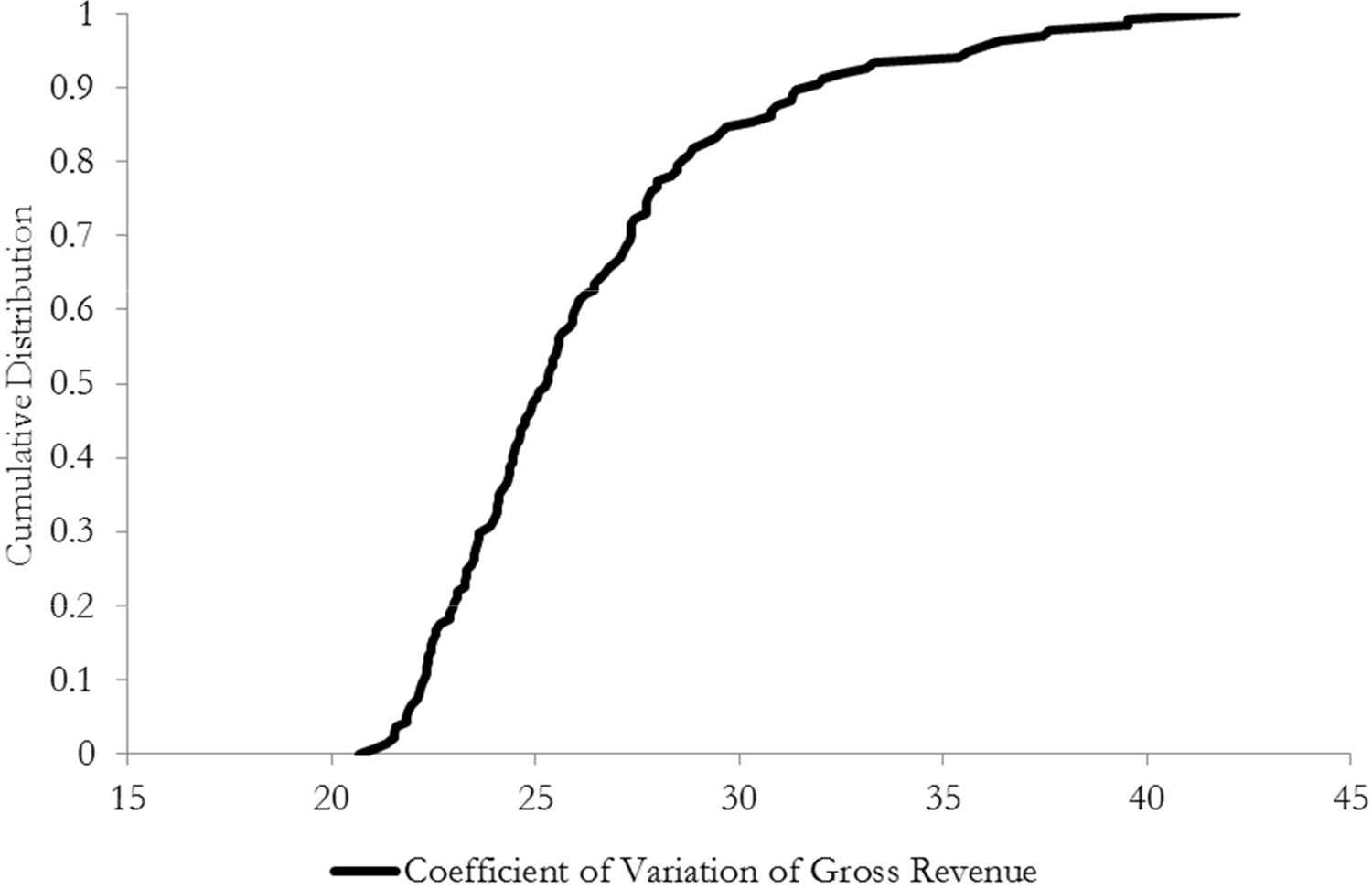
Cumulative distribution of the variability in market gross revenue.
One can see from Figure 6 that the median farmer has an estimated variability in market gross revenue of approximately 25 per cent. None of the 138 farms have an estimated variability of less than twenty per cent while the estimated variability exceeds 30 per cent for approximately 15 per cent of farmers in the sample.
The deduction of direct costs from the Total Gross Revenue allows us to estimate the coefficient of variation for the Market Gross Margin. The coefficient of variation for the Market Gross Margin is higher than for the Market Gross Revenue mainly because a smaller denominator applies to the latter. The average Market Gross Margin is typically much lower than the Gross Revenue due to the costs of production.
In addition, there are a small number of instances of negative Gross Margins. We therefore present the results detailing the coefficient of variation and the standard deviation for different points in the distribution of income variability. The 25th percentile represents the income variability of the farm with the 35th lowest variability among the 138 farms. The 75th percentile represents the income variability of the farm with the 35th highest variability among the 138 farms. One can see from Table 3A that the variability of Gross Margin is approximately 70 per cent for the median farmer. This rises to 119 per cent for the 75th percentile. The 25th percentile has a coefficient of variation in the region of 55 per cent so the variability of profits or Gross Margin is relatively high across most of the distribution.
The variability of market gross margin across the distribution.
| Coefficient of Variation | Standard Deviation | |||||
|---|---|---|---|---|---|---|
| 25th Percentile | Median | 75th Percentile | 25th Percentile | Median | 75th Percentile | |
| Market Gross Revenue | 23.31 | 25.25 | 27.76 | 1780.08 | 3420.50 | 6524.20 |
| Market Gross Margin | 54.96 | 69.77 | 119.43 | 1811.45 | 3531.71 | 6556.58 |
Impact of forward contracts
Having established some estimate of the income variability attached to spring barley production, we now assess the potential impact of forward contracts on reducing income risk and variability. This represents the first attempt in the microsimulation literature to model the role of forward contracts or other financial risk management tools in dealing with risk in agriculture. We include the results both in terms of the coefficient of variation and the standard deviation. In Table 3B, we show that if all farmers in the sample decide to forward sell 20 per cent of production at 150 euro per tonne, the estimated variability (coefficient of variation) drops to 62 per cent for the median case. This reduces further to 57 per cent if all farmers commit 35 per cent of expected production to forward contracts.
For the 75th percentile, the degree of income variability falls but remains at a very elevated level.6
Effect of forward contracting on variability of market gross margin.
| Coefficient of Variation (%) | Standard Deviation | |||||
|---|---|---|---|---|---|---|
| 25th Percentile | Median | 75th Percentile | 25th Percentile | Median | 75th Percentile | |
| Market Gross Margin | 54.96 | 69.77 | 119.43 | 1811.45 | 3531.71 | 6556.58 |
| Margin with Forward Selling Option A | 48.04 | 62.32 | 112.57 | 1639.82 | 3195.35 | 5474.91 |
| Margin with Forward Selling Option B | 42.11 | 57.20 | 97.93 | 1433.87 | 2812.42 | 4703.06 |
-
A-20% of expected production @ 150 euro per tonne B-35% of expected production @ 150 euro per tonne.
In Table 4, we show that the coefficient of variation for the total farm gross margin (excluding subsidies) was, on average, approximately 40 per cent for tillage farmers in the 2005–2013 period. This suggests that tillage farmers manage to reduce their overall farm income variability through the direct government payments and the engagement in livestock farming. Although forward contracting can reduce income variability by approximately twenty per cent, it is likely that tillage farmers find other non-financial risk management tools helpful in containing their income variability and exposure to risk.
Average coefficient of variation by farm system 2005–20137.
| Farm system | Total Farm Gross Margin (%) | Total Farm Gross Margin (Excluding Subsidies) (%) |
|---|---|---|
| Cattle | 28.75 | 57.29 |
| Specialist Dairy | 22.70 | 29.89 |
| Specialist Tillage | 23.86 | 42.38 |
| Sheep | 22.16 | 64.92 |
| Dairy and Other | 25.85 | 50.00 |
| Total | 26.23 | 52.20 |
| Non-Specialist Tillage8 | 21.49 | 39.16 |
| No. of observations | 927 | 927 |
-
Source: Authors calculations using Teagasc National Farm Survey data.
In particular, it appears from Table 5 that a relatively weak positive correlation exists between crop and livestock returns for the majority of farms. We find that the correlation coefficient between the livestock gross margin per hectare and the crop gross margin per hectare is approximately 0.13 for the median case. At the 25th percentile, the correlation coefficient is approximately -0.16 while at the 75th percentile, the correlation coefficient is close to 0.39. These estimates are based on the Teagasc National Farm Survey data for the producers of spring barley for animal feed usage between 1996 and 2013. The results are highly robust to the exclusion of non-specialist cereal producers.
The relatively low correlation between crop and livestock returns suggests that livestock farming can offer some form of risk management for cereal producers. The vast majority of production of spring barley for animal feed usage is sold by the farmer rather than used as feed for their own particular farm. Based on the Teagasc National Farm Survey data, we can report that the share of production sold is above 90 per cent in all years from 2004 to 2013. One may consider the transfer of production from sales to own farm consumption as a form of risk management but it does not appear to be particularly widespread and therefore offers limited protection from adverse price outcomes.
Correlation coefficient between livestock and crop returns.
| Percentile | Correlation Coefficient |
| 10th Percentile | −0.46 |
| 25th Percentile | −0.16 |
| 50th Percentile (Median) | 0.13 |
| 75th Percentile | 0.39 |
| 90th Percentile | 0.61 |
-
Source: Authors calculations using Teagasc National Farm Survey data.
6. Conclusion
In this paper, we have utilised historical farm-level data from the Teagasc National Farm Survey to develop a stochastic microsimulation model for the production of Spring Barley for animal feed use among Irish farmers. This has provided us with an indication of the income risk associated with the production of this grain crop. Forward Contracting is the main available financial risk management tool in Irish tillage farming and we have estimated the first round direct impact of this tool on the variability of profits. The paper is quite a unique contribution as it brings together microsimulation techniques and financial risk management tools to an agricultural setting.
Our results confirm that there is substantial income risk associated with tillage production in Ireland and that a sole focus on tillage production can leave farmers highly vulnerable to market and production risks. Domestic crop prices appear to be largely determined by international forces and domestic crop yields appear to have little influence on domestic crop prices. This means that instances of poor domestic crop yields and disappointing output prices can occur with greater frequency than in larger crop-producing regions or countries, thus leaving Irish farmers more exposed to income risk than their counterparts operating in larger markets.
The relatively high single farm payments therefore play an important role as a risk management tool although this comes with costs for taxpayers and wider society. The forward contracting risk management tool can provide an alternative source of risk management and our results suggest that this tool can reduce the standard deviation of returns by approximately twenty per cent although this is dependent on the share of production committed to the contract.
Although our models have some relatively strong assumptions, the work can support a better understanding about the economic risks associated with the production of grain crops in Ireland and the extent to which forward contracting can offer protection from adverse economic shocks. Farmers will need to establish their own stochastic budgets before considering the forward contracting tool. As in the case of other European farmers, the Irish tillage farmers could benefit from a wider range of available risk management tools. This may include tools capable of giving better protection from adverse changes to the gross margin than is available under a forward contract. Demand for these tools may well be influenced by the degree of dependency on the single farm payment. Future work will incorporate the role of the single farm payments and off-farm work in stabilising household income particularly for these less cost competitive tillage producers. The model can be developed further to examine the potential effect of other risk management tools on income risk including a farm management deposit scheme or gross margin insurance.
The improved management of farm income variability can contribute towards stability in household consumption, support for farm investments, further investment in child education and a reduction in the mental stress associated with variable incomes and therefore is an important issue for policy makers. The findings from this research can facilitate more effective policy design and implementation in this regard. Our results confirm the important role of decoupled direct payments in insulating farmers’ incomes against risk. However, our findings also indicate that income variability has increased in recent years and hence the need for risk management tools. We find that forward contracting can be an effective means of reducing farmers’ exposure to income variability. Whilst forward contracting is not a policy tool, there is a role for policy makers in relation to education and promotion and in the provision of timely, accessible market information, similar to the data provided in the Milk Market Observatory, co-ordinated by the European Commission. Furthermore, our research has examined the relative contribution of price and yield to margin volatility thus providing policy makers with useful information on the source of risk which can support the design of more effective policies, such as the income stabilisation tool for example. Whilst, this paper did not specifically examine the impact of the income stabilisation tool, the modelling infrastructure built as part of this paper could be used in future work to examine this research question.
Intra-temporal correlation matrix.
| Yields | Prices | |||||||||||||
|---|---|---|---|---|---|---|---|---|---|---|---|---|---|---|
| IR | UK | USA | IR | |||||||||||
| Malt | Feed | Mill | Feed | Mill | Feed | |||||||||
| Oats | Barley | Wheat | Barley | Oats | Rye | Wheat | Soybean | Barley | Wheat | Oats | ||||
| IR Oats Yield | 1 | 0.72 | 0.69 | 0.23 | 0.03 | −0.09 | 0.22 | −0.20 | 0.18 | −0.03 | −0.03 | −0.02 | −0.04 | −0.12 |
| IR Barley Yield | 1 | 0.84 | 0.24 | −0.02 | −0.07 | 0.27 | −0.05 | 0.20 | 0.10 | 0.01 | 0.12 | 0.09 | 0.09 | |
| IR Wheat Yield | 1 | 0.24 | 0.33 | −0.16 | 0.51 | −0.04 | 0.05 | −0.10 | −0.20 | −0.08 | −0.13 | −0.11 | ||
| UK Barley Yield | 1 | 0.54 | 0.60 | 0.65 | 0.00 | −0.11 | −0.09 | −0.09 | −0.14 | −0.04 | −0.08 | |||
| UK Oats Yield | 1 | 0.23 | 0.69 | −0.09 | −0.22 | −0.19 | −0.27 | −0.19 | −0.19 | −0.17 | ||||
| UK Rye Yield | 1 | 0.51 | 0.29 | −0.40 | −0.35 | −0.24 | −0.44 | −0.30 | −0.33 | |||||
| UK Wheat Yield | 1 | −0.21 | −0.17 | −0.23 | −0.23 | −0.34 | −0.20 | −0.25 | ||||||
| USA Soybean Yield | 1 | −0.59 | −0.46 | −0.47 | −0.37 | −0.47 | −0.32 | |||||||
| Price IR Malt Barley | 1 | 0.85 | 0.83 | 0.81 | 0.86 | 0.78 | ||||||||
| Price IR Feed Barley | 1 | 0.95 | 0.97 | 0.99 | 0.97 | |||||||||
| Price IR Mill Wheat | 1 | 0.91 | 0.94 | 0.88 | ||||||||||
| Price IR Feed Wheat | 1 | 0.96 | 0.97 | |||||||||||
| Price IR Mill Oats | 1 | 0.96 | ||||||||||||
| Price IR Feed Oats | 1 | |||||||||||||
Footnotes
1.
Assumed that average of the first three months is the relevant price index.
2.
We make this assumption for a number of reasons. For a model of national-level barley production, the number of hectares could be assumed to be a function of a moving average of recent output prices or gross margins. This method has major limitations at the farm-level given the individual farm-level land constraints and the competition between alternative crops and farm activities for land.
3.
Set-aside was initially introduced in order to limit the production of cereals in the EU. It was applied on a voluntary basis from 1988/89. The policy reforms in 1992 made it obligatory as price support became conditional on arable farmers committing a fixed percentage of arable land to set aside. This policy was abolished in 2007/2008.
4.
According to the microdata, it appears that from 2004-2013 that a minority of producers recorded the production of spring barley for both animal feed and malting spring barley in the same year. However, the vast majority of farms with a record of producing malting spring barley have recorded production for both barley types during the course of their participation in the Teagasc National farm Survey. The small sample size of malting barley growers in the Teagasc National Farm Survey means that we do not report precise estimates for this subgroup of farmers.
5.
The average tillage farmer is assumed to have an expected farm income of approximately 33,229. This is based on the size of the lagged decoupled payments and the average coupled income in recent years.
6.
We do not simulate shares of production greater than 35 per cent as there is a risk that the farmer will not be in a position at harvest time to deliver the required quantity on the contract.
7.
One observation is deleted as the coefficient of variation exceeds five.
8.
These farms are engaged in cereal production but are excluded from the Specialist tillage category and are primarily engaged in livestock and/or milk production
References
-
1
What Is Driving Food Prices in 2011?.What Is Driving Food Prices in 2011?. , Oak Brook, Farm Foundation, Issue Reports, IL, USA.
-
2
http://cereals.ahdb.org.uk/markets.aspxUK (LIFFE) Feed Wheat Futures Market Prices.
-
3
Economic performance of alternative tillage systems in the northern corn beltAgronomy Journal 101:296–304.
-
4
http://www.agriculture.gov.au/agriculture-food/drought/assistance/fmd/statisticsFarm Management Deposits Statistics.
-
5
http://www.agriculture.gov.au/ag-farm-food/drought/assistance/fmdFarm Management Deposits Statistics.
-
6
The potential to reduce the risk of diffuse pollution from agriculture while improving economic performance at farm levelEnvironmental Science and Policy 25:118–126.
-
7
On the role of risk versus economies of scope in farm diversification with an application to Ethiopian farmsJournal of Agricultural Economics 63:25–55.
-
8
A stochastic analysis of the decision to produce biomass crops in IrelandBiomass and Bioenergy 46:353–365.
-
9
Understanding the economic factors influencing farm policy preferencesReview of Agricultural Economics 24:309–321.
-
10
Does risk management matter? Evidence from the U.S. agricultural industryJournal of Financial Economics 109:419–440.
-
11
http://www.cso.ie/en/media/csoie/releasespublications/documents/agriculture/2010/full2010Census of Agriculture 2010 - Final Results”. Accessed November 26, 2014.
-
12
Proposal for a Regulation of the European Parliament and of the Council on Support for Rural Development by the European Agricultural Fund for Rural Development (EAFRD), European Commission, Brussels, C0M(2011), 627/3 (2011)Proposal for a Regulation of the European Parliament and of the Council on Support for Rural Development by the European Agricultural Fund for Rural Development (EAFRD), European Commission, Brussels, C0M(2011), 627/3 (2011).
- 13
-
14
Stochastic Partial Equilibrium Modelling: An Application to Crop Yield VariabilityIn: C Zopounidis, N Kalogeras, K Mattas, G van Dijk, G Baourakis, editors. Agricultural Cooperative Management and Policy. Switzerland: Springer International Publishing. pp. 41–61.
-
15
A note on the effects of the Income Stabilisation Tool on income inequality in agricultureJournal of Agricultural Economics 65:739–745.
-
16
Alternative Specifications of Reference Income Levels in the Income Stabilization ToolIn: C Zopounidis, N Kalogeras, K Mattas, G van Dijk, G Baourakis, editors. Agricultural Cooperative Management and Policy. Switzerland: Springer International Publishing. pp. 65–85.
-
17
Stochastic simulation of the cost of home-produced feeds for ruminant livestock systemsJournal of Agricultural Science 150:123–139.
-
18
The Growth Of The Federal Crop Insurance Program, 1990-2011American Journal of Agricultural Economics 95:482–88.
-
19
Determinants of endogenous price risk in corn and wheat futures marketsJournal of Futures Markets 20:753–774.
-
20
Modeling price and yield riskIn: R Just, R Pope, editors. A comprehensive assessment of the role of risk in US agriculture. Norwell, Boston, MA: Kluwer Academic Publisher. pp. 289–324.
-
21
What Harm Is Done By Subsidizing Crop Insurance?American Journal of Agricultural Economics 95:489–497.
-
22
Policy instruments in the common agricultural policyWest European Politics 33:22–38.
-
23
Budgetary and producer welfare effects of revenue insuranceAmerican Journal of Agricultural Economics 79:1024–1034.
-
24
Quantifying the viability of farming in Ireland: can decoupling address the regional imbalances?Irish Geography 41:29–47.
-
25
Forty years of the Common Agricultural Policy: The Irish farming experienceAdministration 62:87–102.
-
26
The development of farm-level sustainability indicators for Ireland using the Teagasc National Farm SurveyIreland: Teagasc.
-
27
Possible change in Irish climate and its impact on barley and potato yieldsAgricultural and Forest Meteorology 116:181–196.
- 28
-
29
Building a static farm level spatial microsimulation model for rural development and agricultural policy analysis in IrelandInternational Journal of Agricultural Resources, Governance and Ecology 8:282–299.
-
30
Farm income variability and offfarm diversification among Canadian farm operatorsAgricultural Finance Review 71:329–346.
-
31
Grain yield reductions in spring barley due to barley yellow dwarf virus and aphid feedingIrish Journal of Agricultural and Food Research 44:111–128.
- 32
-
33
The profit impacts of risk management tool adoptionAgricultural Finance Review 72:104–116.
-
34
The capacity to expand milk production in Ireland following the removal of milk quotasIrish Journal of Agricultural and Food Research 51:1–11.
-
35
An ex-ante assessment of CAP income stabilisation payments using a farm house hold model, in 87th annual conference of the agricultural economics societyUK, University of Warwick.
-
36
Responsiveness of Crop Yield and Acreage to Prices and ClimateAmerican Journal of Agricultural Economics 97:1–21.
-
37
Nowcasting indicators of poverty risk in the European Union: a microsimulation approachSocial Indicators Research 119:101–119.
-
38
The simultaneous hedging of price risk, crop yield risk and currency riskCanadian Journal of Agricultural Economics/Revue canadienne d’agroeconomie 48:123–140.
-
39
Modelling Farm ViabilityIn: C O’Donoghue, D Ballas, G Clarke, S Hynes, K Morrissey, editors. Spatial Microsimulation for Rural Policy Analysis. Springer Berlin Heidelberg. pp. 177–191.
- 40
- 41
-
42
Analysis of environmental and economic efficiency using a farm population micro-simulation modelMathematics and Computers in Simulation 81:1344–1352.
-
43
An applied procedure for estimating and simulating multivariate empirical (MVE) probability distributions in farm-level risk assessment and policy analysisJournal of Agricultural and Applied Economics 32:299–316.
-
44
Simulation and Econometrics to Analyze RiskDepartment of Agricultural Economics, Texas A and M University.
-
45
Farm Level Models’In: Cathal O’Donoghue, editors. Handbook of Microsimulation Modelling, (Contributions to Economic Analysis 293). Emerald Group Publishing Limited. pp. 505–534.
-
46
Optimal procurement strategies for online spot marketsEuropean Journal of Operational Research 152:781–799.
-
47
Description and validation of the Moorepark Dairy Systems ModelJournal of Dairy Science 87:1945–1958.
-
48
The Effect of Decoupling on Farming in Ireland: A Regional AnalysisIrish Journal of Agriculture and Food Research 46:1–13.
- 49
-
50
http://www.teagasc.ie/publications/2013/30437ReviewAndOutlook2014.pdfReview of Tillage Farming in 2013 and Outlook for 2014 in Teagasc Outlook 2014, 35–64.
- 51
Article and author information
Author details
Acknowledgements
The authors acknowledge the funding support of the Department of Agriculture, Food and the Marine under the project entitled ‘Volatility and Risk in Irish Agriculture’. The authors acknowledge the training provided by the FAPRI (Food and Agricultural Policy Research Institute) Missouri team in delivering a short course in Partial Equilibrium Modeling at the FAPRI Institute in July 2014 in Columbia, Missouri, USA.
Publication history
- Version of Record published: August 31, 2016 (version 1)
Copyright
© 2016, Loughrey
This article is distributed under the terms of the Creative Commons Attribution License, which permits unrestricted use and redistribution provided that the original author and source are credited.