Estimating and simulating with a random utility random opportunity model of job choice. Presentation and application to Belgium
- Department of Economics, KU Leuven, Belgium
- Federal Planning Bureau, Belgium
- Article
- Figures and data
- Jump to
Figures

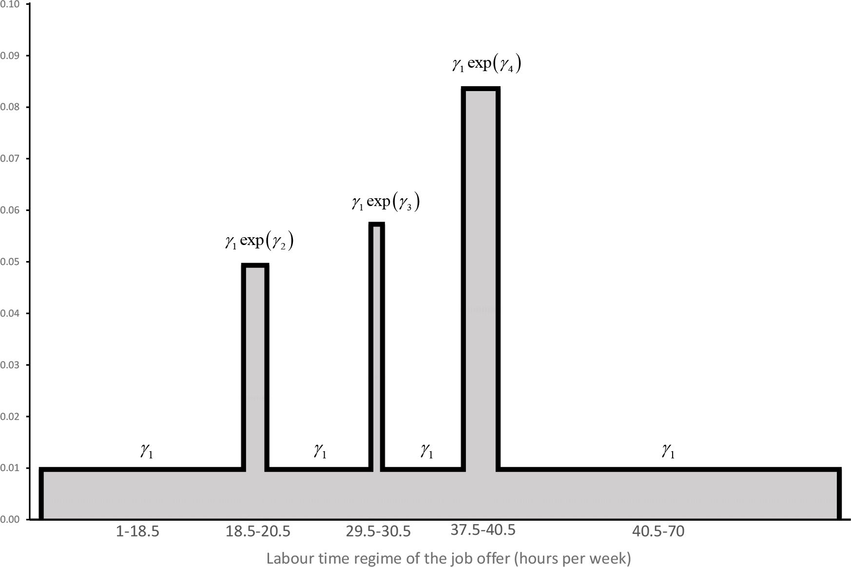
Peak distribution for labour time regimes.

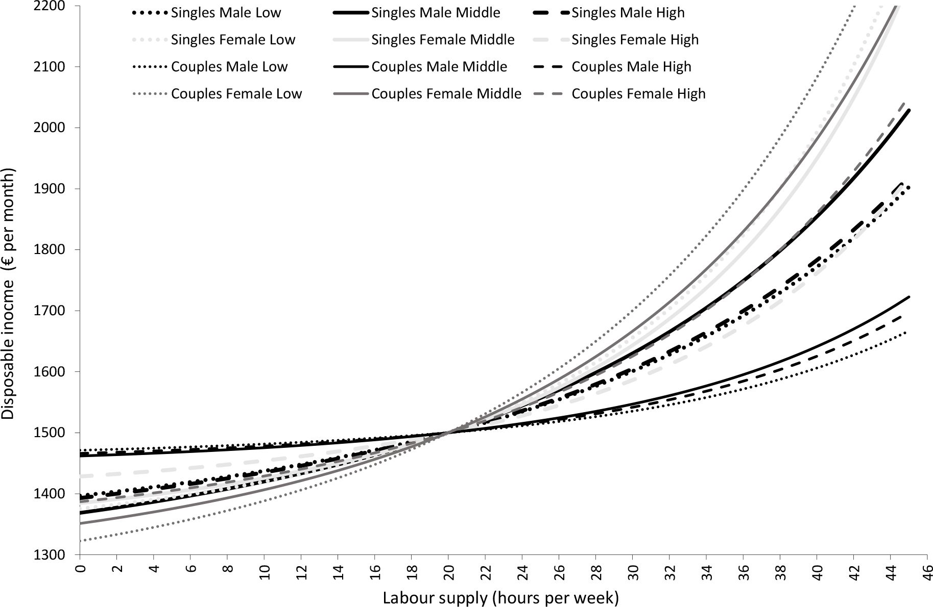
Impact of education level on steepness of indifference curves.

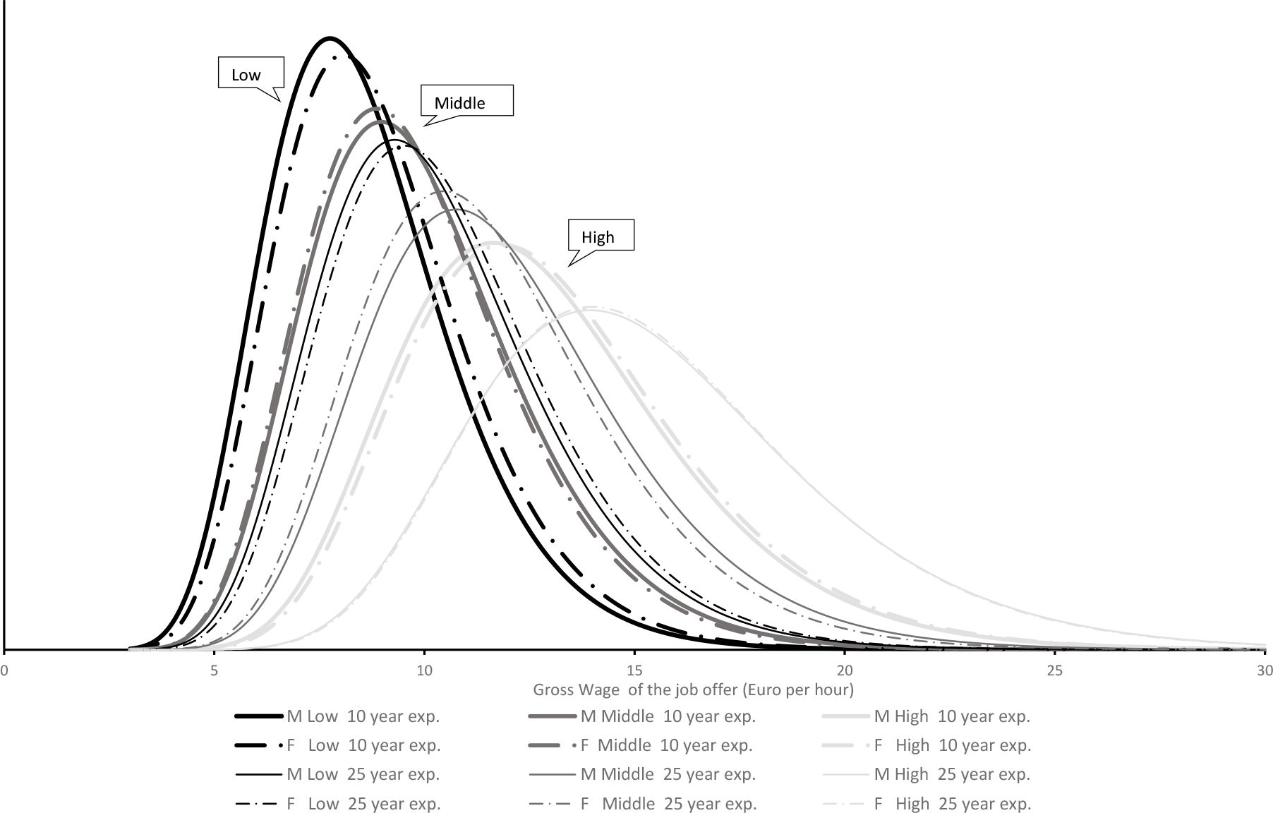
Estimated wage offer distributions and education.

Estimated distribution of offered labour time regimes.

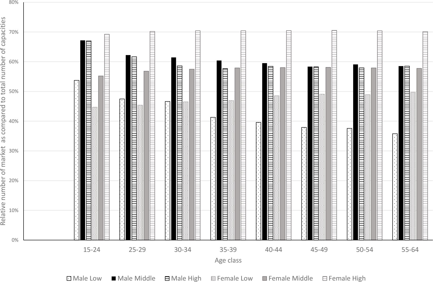
Job offer intensity in function of education and age specific unemployment rate.
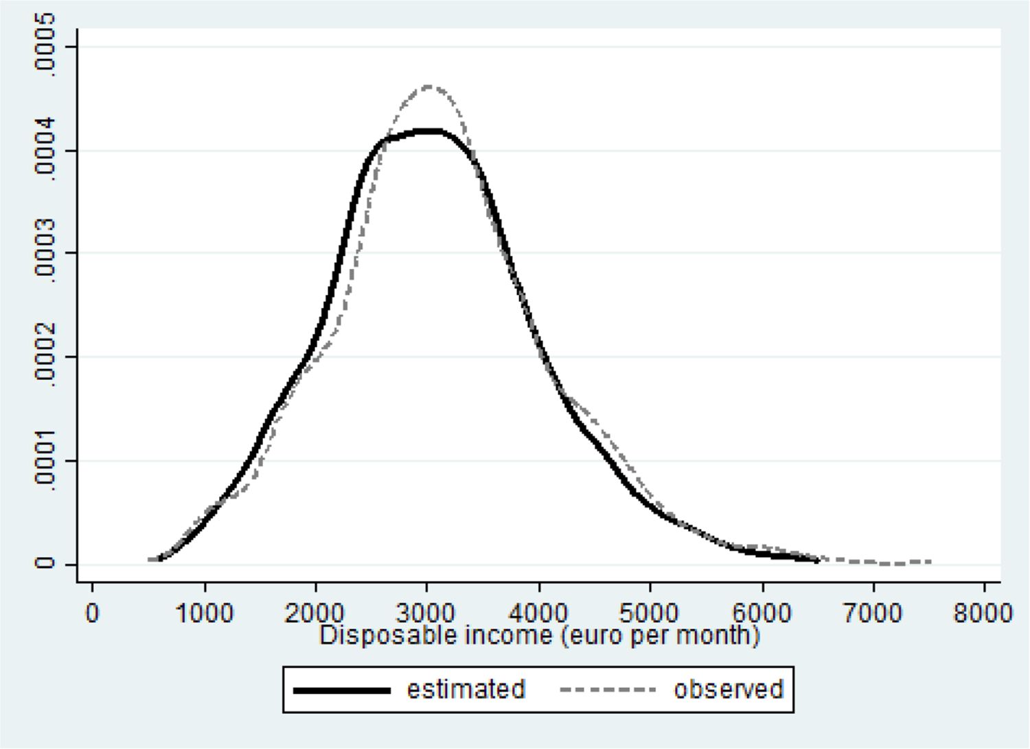
Fit disposable income for couples.

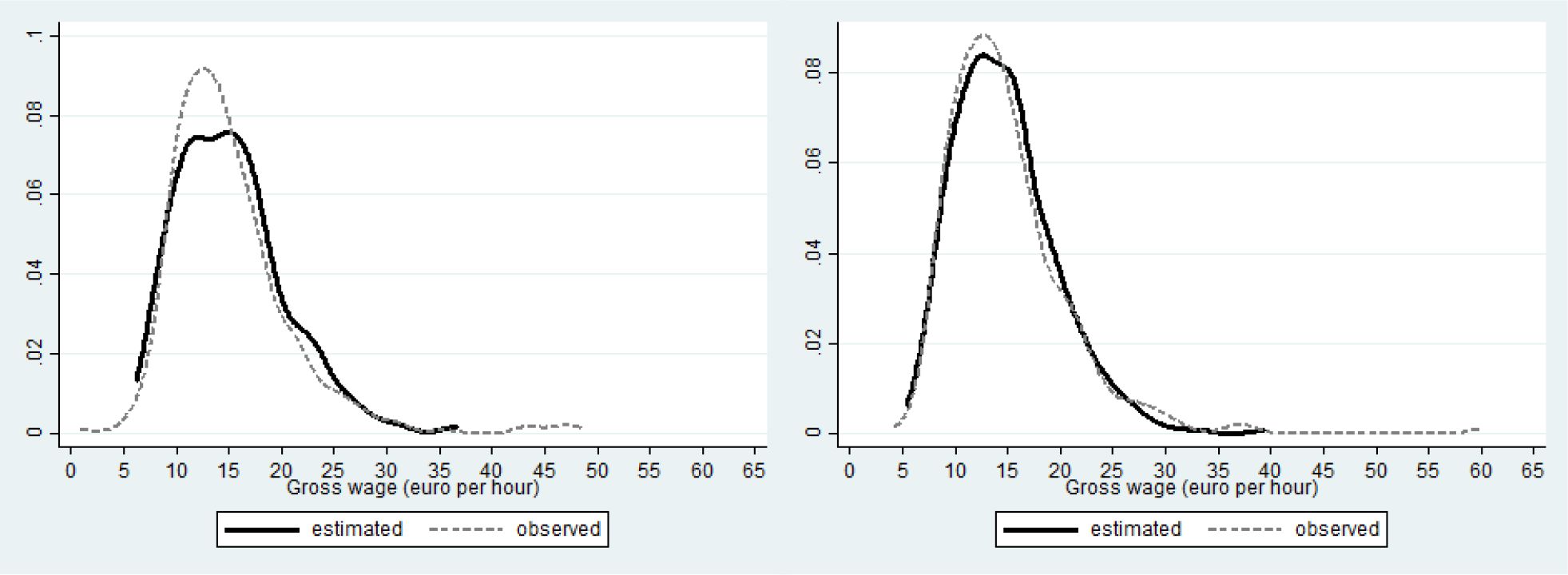
Fit wages males (left) and females (right) in couples.
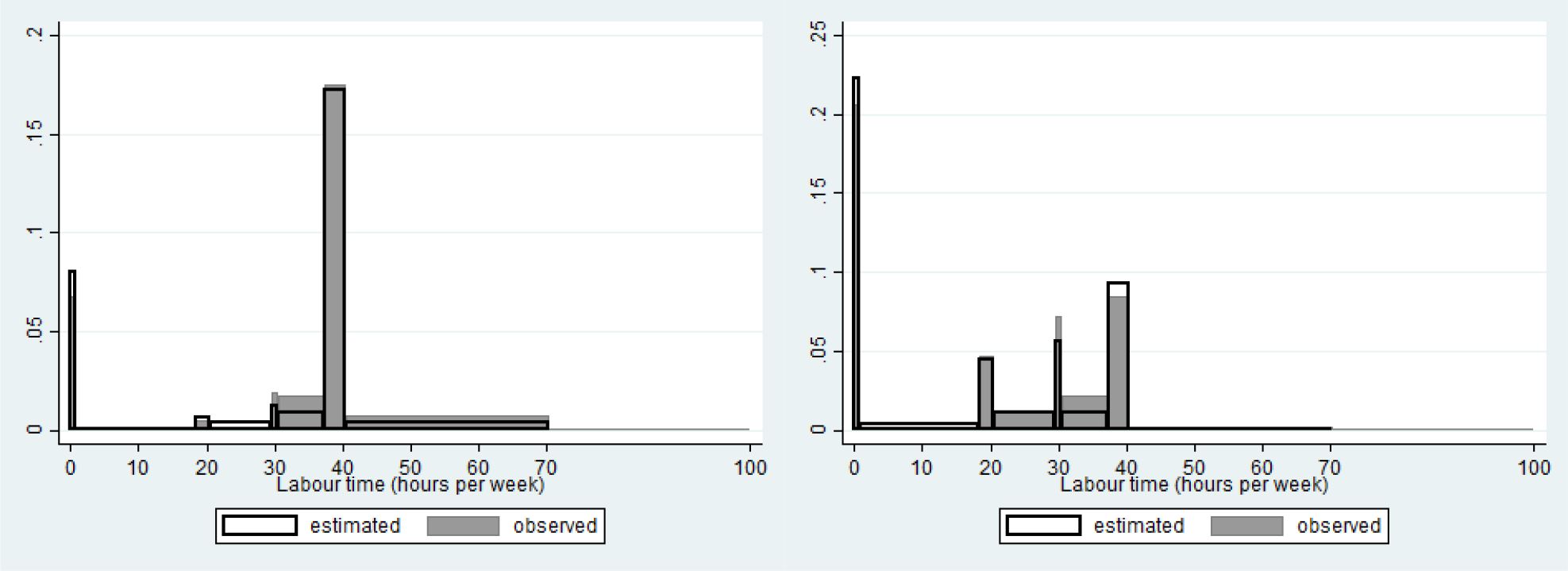
Fit labour time males (left) and females (right) in couples.
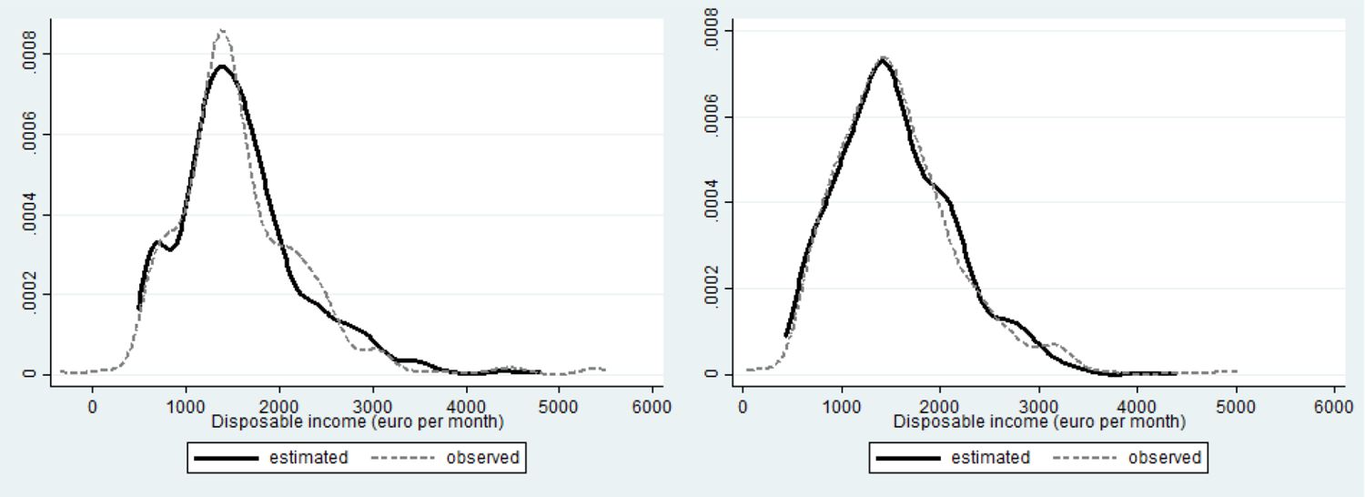
Fit disposable income single males (left) and single females (right).

Fit wages single males (left) and females (right).

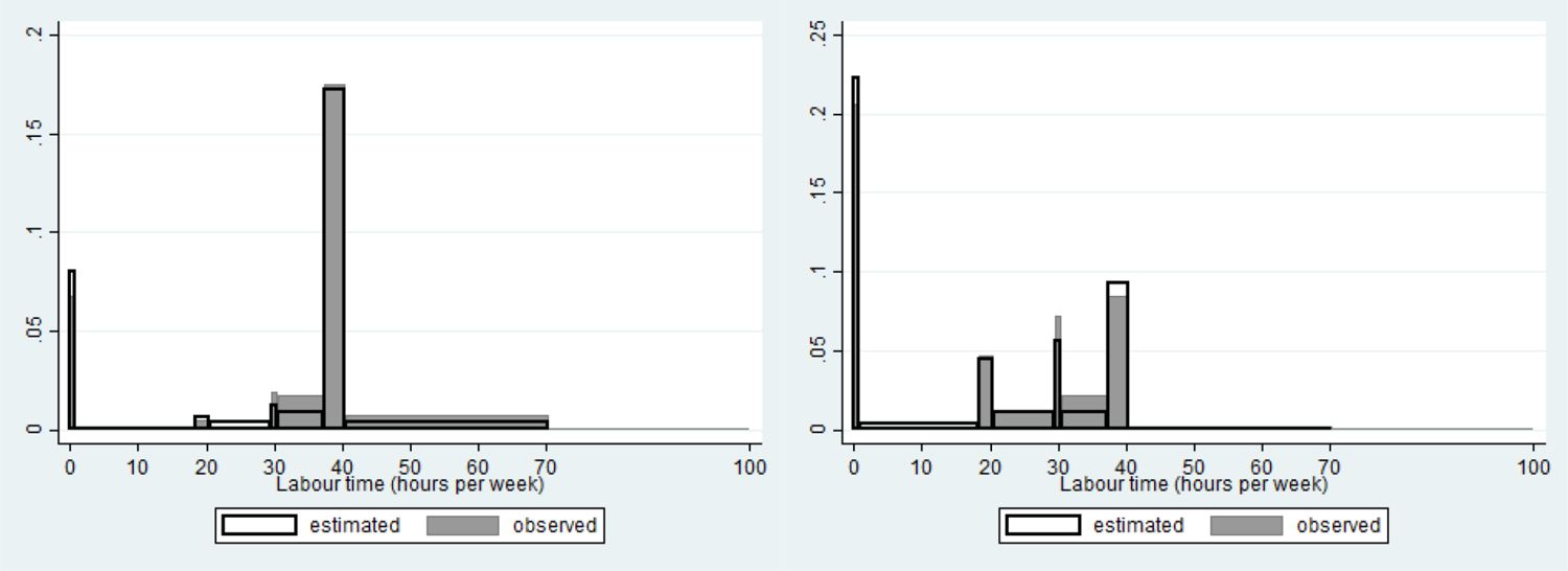
Fit labour time regimes single males (left) and single females (right).
Tables
Descriptive statistics for the estimation sample.
| Singles | Couples | |||
|---|---|---|---|---|
| Description | Female | Male | Female | Male |
| Age (years) | 41.1 | 39.93 | 38.08 | 40.22 |
| % hh having 0–3 year old children | 5.78% | 0.45% | 18.67% | |
| % hh having 4–6 year old children | 9.46% | 0.89% | 17.16% | |
| % hh having 7–9 year old children | 10.16% | 1.78% | 18.19% | |
| Education: | ||||
| Lowly educated | 22.8% | 24.5% | 16.8% | 19.8% |
| Secondary education | 34.6% | 41.9% | 38.5% | 39.0% |
| Highly educated | 42.6% | 33.6% | 44.7% | 41.2% |
| Residence: | ||||
| Brussels | 19.8% | 21.2% | 9.3% | |
| Flanders | 44.1% | 45.2% | 58.5% | |
| Wallonia | 36.1% | 33.6% | 32.3% | |
| Participation rate (%) | 68.12 | 78.84 | 79.40 | 93.20 |
| Hours worked/week: | ||||
| Conditional on working | 35.88 | 39.69 | 32.50 | 40.84 |
| Unconditional | 24.45 | 31.29 | 25.81 | 38.06 |
| Hourly wage (euro) | 14.91 | 15.20 | 14.73 | 16.25 |
| Disposable income (€ /month) | 1567 | 1588 | 3143 | |
| Number of observations | 571 | 449 | 1457 | |
-
Source: Own Calculations, eu-silc 2007.
Type specific unemployment rates (%).
| Male | Female | |||||
|---|---|---|---|---|---|---|
| Education level | Education level | |||||
| Age group | Low | Middle | High | Low | Middle | High |
| 15 to 24 years | 26.4 | 14.0 | 12.3 | 33.6 | 22.1 | 11.0 |
| 25 to 29 years | 19.0 | 7.6 | 6.9 | 29.7 | 13.1 | 4.8 |
| 30 to 34 years | 18.0 | 6.6 | 3.1 | 23.5 | 9.3 | 3.3 |
| 35 to 39 years | 11.6 | 5.3 | 2.0 | 21.2 | 6.9 | 3.2 |
| 40 to 44 years | 9.5 | 4.2 | 2.9 | 12.2 | 6.2 | 3.0 |
| 45 to 49 years | 7.4 | 2.8 | 2.7 | 9.3 | 5.8 | 2.4 |
| 50 to 54 years | 7.0 | 3.7 | 2.3 | 10.1 | 7.0 | 3.5 |
| 55 to 64 years | 4.7 | 3.0 | 3.0 | 5.8 | 7.8 | 5.3a |
-
a
The exact figure is lacking. The average across all education levels for that age class is taken.
-
Source: Eurostat unemployment rates by sex, age and educational attainment level (%), Belgium 2007, http://appsso.eurostat.ec.europa.eu/nui/show.do?dataset=lfsa_urgaed&lang=en, downloaded in October 2013.
Model specification.
| Preferences | Opportunities | |||
|---|---|---|---|---|
| xV | xopp | xh | xw | |
| variable | job offers | hours | wages | |
| Regional dummiesa | yes | yes | no | no |
| Education dummiesb | yes | yes | no | yes |
| Age | yes | no | no | no |
| Group specific unemployment rate | no | yes | no | no |
| Number of children | yes | no | no | no |
| Gender | yes | yes | yes | yes |
| Potential experience | no | no | no | yes |
-
a
Brussels, Flanders, Wallonia.
-
b
Low, Middle, High.
Aggregate wage elasticity of labour supply.
| Shift of female wage distribution | Shift of male wage distribution | |||||
|---|---|---|---|---|---|---|
| Couple | Single | Couple | Single | |||
| Female | Male | Female | Male | Female | Male | |
| Total elasticity | 0.6445 | -0.1734 | 0.6877 | -0.2014 | 0.3304 | 0.4569 |
| Intensive margin | 0.2162 | -0.2222 | 0.1257 | -0.2584 | 0.1365 | 0.0944 |
| Part in | 3.157% | 0.480% | 3.327% | 0.549% | 1.716% | 2.895% |
| Part out | 0.000% | 1.647% | 0.000% | 1.579% | 0.000% | 0.000% |
Education level distribution by age and sex.
| Education level | Low | Middle | High | |||
|---|---|---|---|---|---|---|
| Scenario | baseline | counterfactual | baseline | counterfactual | baseline | counterfactual |
| Age | males | |||||
| 15 – 25 | 21.20% | 20.10% | 40.15% | 39.90% | 38.65% | 39.99% |
| 26 – 30 | 27.42% | 19.84% | 41.27% | 40.00% | 31.31% | 40.16% |
| 31 – 35 | 27.27% | 19.44% | 40.41% | 40.13% | 32.32% | 40.43% |
| 36 – 40 | 27.66% | 20.47% | 40.22% | 39.75% | 32.11% | 39.78% |
| 41 – 45 | 26.87% | 19.80% | 39.22% | 40.24% | 33.92% | 39.96% |
| 46 – 50 | 26.62% | 20.33% | 39.68% | 39.97% | 33.71% | 39.70% |
| 51 – 55 | 26.12% | 20.50% | 38.15% | 39.84% | 35.73% | 39.67% |
| 56 – 60 | 25.35% | 20.15% | 38.79% | 39.95% | 35.86% | 39.90% |
| 61 – 65 | 24.15% | 19.96% | 38.66% | 39.70% | 37.18% | 40.33% |
| all | 27.27% | 20.90% | 41.54% | 41.42% | 31.19% | 37.68% |
| females | ||||||
| 15 – 25 | 20.36% | 20.21% | 40.23% | 40.12% | 39.41% | 39.68% |
| 26 – 30 | 20.22% | 19.51% | 39.77% | 40.38% | 40.01% | 40.11% |
| 31 – 35 | 18.71% | 20.26% | 38.09% | 40.12% | 43.20% | 39.62% |
| 36 – 40 | 19.77% | 19.31% | 38.35% | 39.69% | 41.89% | 41.00% |
| 41 – 45 | 19.61% | 20.14% | 38.03% | 39.68% | 42.36% | 40.19% |
| 46 – 50 | 19.35% | 20.46% | 38.27% | 39.58% | 42.38% | 39.96% |
| 51 – 55 | 19.14% | 20.12% | 38.03% | 38.80% | 42.83% | 41.08% |
| 56 – 60 | 20.03% | 19.33% | 38.73% | 40.48% | 41.24% | 40.19% |
| 61 – 65 | 19.46% | 20.11% | 39.01% | 39.80% | 41.53% | 40.09% |
| all | 20.52% | 20.79% | 40.26% | 41.17% | 39.22% | 38.04% |
-
Source: midas implemented scenarios for baseline coinciding with 2007 and counterfactual aiming at a catch-up of female’s higher education level than males’ in the baseline, by 2050.
Participation and mean labour time by age class in baseline and counterfactual.
| Age | 15 – 25 | 26 – 30 | 31 – 35 | 36 – 40 | 41 – 45 | 46 – 50 | 51 – 55 | 56 – 60 | 61 – 65 | all |
|---|---|---|---|---|---|---|---|---|---|---|
| Couples: males | ||||||||||
| n obs | 68 | 182 | 247 | 290 | 243 | 132 | 148 | 90 | 16 | 1457 |
| part baseline | 89.7% | 90.1% | 88.7% | 94.1% | 92.2% | 94.8% | 93.2% | 74.4% | 87.5% | 90.9% |
| part counterf. | 89.7% | 92.3% | 89.1% | 94.5% | 93.4% | 96.0% | 93.2% | 80.0% | 87.5% | 92.0% |
| h baseline | 33.4 | 34.3 | 35.9 | 38.8 | 37.2 | 38.3 | 37.4 | 28.2 | 35.8 | 36.4 |
| h counterf. | 33.4 | 35.1 | 36.2 | 39.0 | 37.6 | 38.6 | 37.2 | 30.2 | 35.8 | 36.7 |
| Couples: females | ||||||||||
| n obs | 124 | 241 | 264 | 260 | 230 | 172 | 99 | 58 | 9 | 1457 |
| part baseline | 74.2% | 78.8% | 73.5% | 78.8% | 82.2% | 80.8% | 73.7% | 72.4% | 55.6% | 77.5% |
| part counterf. | 73.4% | 77.2% | 73.5% | 78.1% | 81.3% | 80.2% | 75.8% | 69.0% | 55.6% | 76.8% |
| h baseline | 24.3 | 25.4 | 23.2 | 24.7 | 26.0 | 24.9 | 20.9 | 22.7 | 18.1 | 24.4 |
| h counterf. | 24.2 | 24.7 | 23.0 | 24.4 | 25.6 | 24.3 | 21.6 | 22.1 | 18.1 | 24.0 |
| Singles: females | ||||||||||
| n obs | 43 | 59 | 83 | 97 | 89 | 82 | 55 | 51 | 12 | 571 |
| part baseline | 58.1% | 69.5% | 69.9% | 66.0% | 65.2% | 79.3% | 80.0% | 70.6% | 50.0% | 69.5% |
| part counterf. | 58.1% | 69.5% | 68.7% | 66.0% | 65.2% | 78.0% | 80.0% | 70.6% | 50.0% | 69.2% |
| h baseline | 18.4 | 23.6 | 27.1 | 23.6 | 21.9 | 27.1 | 24.8 | 21.8 | 14.3 | 23.7 |
| h counterf. | 18.4 | 23.6 | 26.6 | 23.6 | 21.9 | 26.8 | 24.8 | 21.8 | 14.3 | 23.6 |
| Singles: males | ||||||||||
| n obs | 46 | 60 | 67 | 68 | 54 | 65 | 46 | 33 | 10 | 449 |
| part baseline | 80.4% | 88.3% | 91.0% | 77.9% | 85.2% | 87.7% | 67.4% | 72.7% | 50.0% | 80.6% |
| part counterf. | 80.4% | 83.3% | 92.5% | 85.3% | 87.0% | 87.7% | 69.6% | 72.7% | 60.0% | 83.1% |
| h baseline | 31.5 | 30.3 | 34.6 | 30.0 | 32.8 | 33.2 | 23.3 | 25.2 | 18.5 | 30.4 |
| h counterf. | 31.5 | 32.1 | 35.1 | 34.2 | 33.6 | 33.3 | 24.7 | 25.2 | 22.1 | 31.7 |
Impact of education through preferences and opportunities.
| Couple | Single | |||
|---|---|---|---|---|
| Males | Females | Males | Females | |
| n obs | 1457 | 1457 | 449 | 571 |
| part base | 90.87% | 77.48% | 80.62% | 69.53% |
| part alt pref | 90.94% | 77.62% | 81.51% | 69.53% |
| part alt opp | 91.90% | 76.94% | 82.85% | 69.35% |
| part counterf. | 91.97% | 76.80% | 83.07% | 69.17% |
| h base | 36.35 | 24.35 | 30.37 | 23.72 |
| h alt pref | 36.27 | 24.32 | 30.82 | 23.72 |
| h alt opp | 36.78 | 24.12 | 31.38 | 23.67 |
| h counterf. | 36.73 | 24.04 | 31.67 | 23.60 |
Preferences couples.
| Log likelihood | −8482.1758 | ||
|---|---|---|---|
| Description | Estimate | Standard Error | t-value |
| 1.a) Consumption & leisure interaction M&F | |||
| Consumption Couples exponent | 0.610 | 0.051 | 11.96 |
| Consumption Couples constant | 4.873 | 0.310 | 15.70 |
| Leisure interaction M&F.in couples | 0.206 | 0.077 | 2.69 |
| Consumption single M exponent | 0.292 | 0.123 | 2.38 |
| Consumption single M constant | 4.740 | 0.395 | 12.00 |
| Consumption single F exponent | 0.049 | 0.149 | 0.33 |
| Consumption single F constant | 4.181 | 0.338 | 12.36 |
| 1.b) Leisure coefficients males in couples | |||
| Leisure M in couples exponent | −8.351 | 0.663 | −12.59 |
| Leisure M in couples constant | 20.959 | 7.880 | 2.66 |
| Leisure M in couples ln(age) | −11.339 | 4.321 | −2.62 |
| Leisure M in couples ln(age)2 | 1.591 | 0.601 | 2.65 |
| Leisure M in couples ch03 | 0.007 | 0.059 | 0.12 |
| Leisure M in couples ch36 | 0.078 | 0.063 | 1.23 |
| Leisure M in couples ch69 | −0.009 | 0.058 | −0.15 |
| Leisure M in couples dum region Walloona | 0.132 | 0.068 | 1.94 |
| Leisure M in couples dum region Brusselsa | 0.168 | 0.112 | 1.49 |
| Leisure M in couples dum education LOWb | −0.174 | 0.085 | −2.05 |
| Leisure M in couples dum education HIGHb | −0.078 | 0.060 | −1.31 |
| 1.c) Leisure coefficients females in couples | |||
| Leisure F in couples exponent | −6.995 | 0.502 | −13.93 |
| Leisure F in couples constant | 32.068 | 14.700 | 2.18 |
| Leisure F in couples ln(age) | −18.521 | 8.368 | −2.21 |
| Leisure F in couples ln(age)2 | 2.879 | 1.197 | 2.40 |
| Leisure F in couples ch03 | 0.550 | 0.179 | 3.08 |
| Leisure F in couples ch36 | 0.533 | 0.187 | 2.84 |
| Leisure F in couples ch69 | 0.426 | 0.191 | 2.23 |
| Leisure F in couples dum region Walloona | 0.302 | 0.173 | 1.74 |
| Leisure F in couples dum region Brusselsa | 0.062 | 0.247 | 0.25 |
| Leisure F in couples dum education LOWb | 0.612 | 0.331 | 1.85 |
| Leisure F in couples dum education HIGHb | −0.753 | 0.183 | −4.10 |
-
a
Flanders region is reference category.
-
b
Middle education level is reference category.
Preferences singles.
| Description | Estimate | Standard Error | t-value |
|---|---|---|---|
| 1.d) Leisure coefficients single males | |||
| Leisure single M exponent | −5.444 | 1.002 | −5.43 |
| Leisure single M constant | 36.394 | 23.737 | 1.53 |
| Leisure single M ln(age) | −20.375 | 13.239 | −1.54 |
| Leisure single M ln(age)2 | 3.024 | 1.865 | 1.62 |
| Leisure single M ch36 | −0.457 | 1.112 | −0.41 |
| Leisure single M ch69 | −1.135 | 0.698 | −1.63 |
| Leisure single M dum region Walloona | 0.951 | 0.425 | 2.24 |
| Leisure single M dum region Brusselsa | 0.262 | 0.372 | 0.70 |
| Leisure single M dum education LOWb | −0.581 | 0.387 | −1.50 |
| Leisure single M dum education HIGHb | −0.502 | 0.335 | −1.50 |
| 1.e) Leisure coefficients single females | |||
| Leisure single F exponent | −7.688 | 0.977 | −7.87 |
| Leisure single F constant | 62.678 | 23.311 | 2.69 |
| Leisure single F ln(age) | −34.609 | 12.929 | −2.68 |
| Leisure single F ln(age)2 | 4.876 | 1.809 | 2.70 |
| Leisure single F ch03 | 0.838 | 0.502 | 1.67 |
| Leisure single F ch36 | 0.128 | 0.239 | 0.54 |
| Leisure single F ch69 | −0.141 | 0.196 | −0.72 |
| Leisure single F dum region Walloona | 0.212 | 0.199 | 1.06 |
| Leisure single F dum region Brusselsa | −0.258 | 0.188 | −1.37 |
| Leisure single F dum education LOWb | 0.133 | 0.326 | 0.41 |
| Leisure single F dum education HIGHb | −0.616 | 0.217 | −2.84 |
-
a
Flanders region is reference category;
-
b
Middle education level is reference category.
Opportunities, relative intensity of market alternatives, peaks hours, and wage offer distribution.
| Description | Estimate | Standard Error | t-value |
|---|---|---|---|
| 2.a) Estimated coefficients opportunities & peaks males | |||
| Opportunity M constant | −4.488 | 0.247 | −18.19 |
| Opportunity M unemployment rate | 0.338 | 0.226 | 1.50 |
| Opportunity M dummy region Walloona | −0.547 | 0.223 | −2.45 |
| Opportunity M dummy region Brusselsa | −1.215 | 0.285 | −4.27 |
| Opportunity M dummy LOW educationb | −0.987 | 0.277 | −3.56 |
| Opportunity M dummy HIGH educationb | 0.049 | 0.265 | 0.19 |
| Peaks M <18.5,20.5> interval | 0.643 | 0.229 | 2.81 |
| Peaks M <29.5,30.5> interval | 0.862 | 0.189 | 4.55 |
| Peaks M <37.5,40.5> interval | 2.690 | 0.060 | 45.17 |
| 2.b) Estimated coefficients opportunities & peaks females | |||
| Opportunity F constant | −4.300 | 0.185 | −23.19 |
| Opportunity F unemployment rate | −0.072 | 0.124 | −0.58 |
| Opportunity F dummy region Walloona | −0.394 | 0.157 | −2.51 |
| Opportunity F dummy region Brusselsa | −0.783 | 0.219 | −3.58 |
| Opportunity F dummy LOW educationb | −0.339 | 0.217 | −1.56 |
| Opportunity F dummy HIGH educationb | 0.522 | 0.195 | 2.68 |
| Peaks F <18.5,20.5> interval | 1.636 | 0.100 | 16.42 |
| Peaks F <29.5,30.5> interval | 1.804 | 0.108 | 16.69 |
| Peaks F <37.5,40.5> interval | 2.206 | 0.070 | 31.36 |
| 3. Estimated coefficients wage equations | |||
| 3.a) Wage equation males | |||
| Wage M σ | 0.264 | 0.004 | 60.63 |
| Wage M constant | 2.066 | 0.029 | 72.00 |
| Wage M potential experience | 2.297 | 0.244 | 9.41 |
| Wage M potential experience2 | −3.110 | 0.545 | −5.71 |
| Wage M LOW educationb | −0.147 | 0.019 | −7.79 |
| Wage M HIGH educationb | 0.260 | 0.015 | 17.39 |
| 3.b) Wage equation females | |||
| Wage F σ | 0.261 | 0.004 | 59.05 |
| Wage F constant | 2.043 | 0.026 | 77.61 |
| Wage F potential experience | 2.457 | 0.239 | 10.30 |
| Wage F potential experience2 | −3.869 | 0.592 | −6.54 |
| Wage F LOW educationb | −0.095 | 0.023 | −4.08 |
| Wage F HIGH educationb | 0.291 | 0.016 | 18.61 |
-
a
Flanders region is reference category;
-
b
Middle education level is reference category.