Evaluating the quality of gross incomes in SILC: Compare them with fiscal data and re-calibrate them using EUROMOD
- Herman Deleeck Centre for Social Policy, University of Antwerp, Belgium
- Research Centre of Public Economics, Belgium
- Article
- Figures and data
-
Jump to
- Abstract
- 1. Introduction
- 2. Data
- 1.1 Internal validity of SILC incomes
- 1.2 Matching SILC with IPCAL
- 2. Comparing gross incomes in IPCAL and SILC
- 2.1 Total household gross income
- 2.2 Gross income components
- 2.3 Possible explanations for the underreporting of gross incomes in SILC
- 3. Constructing adjusted gross incomes
- 3.1 Methodology
- 3.2 Gross employee income
- 3.3 Gross self-employment income
- 3.4 Gross pension income
- 3.5 Gross unemployment income, sickness and disability benefits
- 4. Comparing new gross incomes in SILC with IPCAL
- 4.1 Total household gross income
- 4.2 Gross income components
- 5. Conclusion
- Footnotes
- References
- Article and author information
Abstract
In this paper, we shed light on the quality of the gross incomes as reported in the Survey on Income and Living Conditions (SILC). This is done in three steps. First, as both net and gross incomes are reported in SILC, implicit tax rates are calculated and evaluated. In a second step, gross incomes from SILC are compared with gross incomes reported on the fiscal form for the same individuals. Finally, we make use of EUROMOD to re-calibrate SILC gross incomes in order to make them consistent with the reported net ones. We find that, on average, fiscally reported gross incomes exceed gross incomes in the SILC survey. It is not clear however whether the re-calibration method (whereby we use an iterative method to construct adjusted SILC gross incomes starting from the observed net ones) is a genuine improvement upon the reported gross income distribution.
1. Introduction
Surveys form the basis for national statistics on poverty, inequality and other socio-economic conditions. As they constitute an important pillar for research and policy making, it is all the more alarming that the quality of surveys seems to be declining (Meyer et al., 2015). They name three reasons for this trend. First, households are increasingly less willing to take part in surveys, leading to an increase in so called unit non-response. Second, they cannot or do not want to provide the answer to specific questions, leading to item non-response. And third, when they do answer, the answer is often inaccurate, leading to measurement error. The growing availability of administrative data fuels the debate on whether or not to supplement selected survey variables with administrative data, or to even replace survey data entirely by administrative data. Proponents argue that such reforms would save up interview time and may lead to more robust results, as administrative data does not suffer from selective non-response and erroneous reporting (Epland, 2006). But administrative data suffers from inherent shortcomings as well, as it cannot take tax evasion into account (in the case of data from tax forms), and they often measure a slightly different concept than the measure from the survey (Abowd & Stinson., 2013, Kapteyn & Ypman, 2007).
Most studies assessing the quality of either survey or administrative data perform a cross-validation exercise, in which a selection of income statistics are compared for the entire population and along the distribution (see e.g. Abowd & Stinson, 2013; Kapteyn & Ypman, 2007; Liégeois et al., 2011; Lohmann, 2007). In this study, the quality of the Survey on Income and Living Conditions (SILC) data is assessed, both measuring the dataset’s internal consistency through a comparison of gross and net incomes, and by comparing gross incomes with their identical match in the administrative (or register) data. We dispose of a unique dataset which combines tax return data (the IPCAL dataset) with survey data for the individuals included in the SILC survey.
The paper is structured as follows: in Section 2, we first describe the survey data and assess the internal consistency of the reported incomes, before describing how the survey data is linked to the tax form data. In Section 3, we compare gross SILC incomes with its administrative counterparts. This comparison reveals that gross incomes in SILC are underreported compared to the ones in the administrative IPCAL data. We then focus on three elements which can (partly) explain this underreporting, that is the imputation of missing values; the source of information used by the respondent and; stability of the socio-economic status throughout the year.
As neither of these elements gives a satisfactory explanation of the mismatch between the SILC and IPCAL gross incomes, we will explore one of several possible routes to adapt gross SILC incomes. It is based on the assumption that SILC respondents might have better knowledge of their net incomes than of their gross ones. In that case it seems natural to start from these reported net incomes to reconstruct ‘corrected’ gross incomes. This method is explained in Section 4. Finally, in Section 5, the distribution of newly calculated SILC gross incomes is compared with the gross incomes from the administrative dataset to check whether an improvement in the correspondence between SILC and IPCAL datasets is notable. Section 6 concludes.
2. Data
The European Union Survey on Income and Living Conditions (EU-SILC), a micro data set with a representative sample of private households, is the standard dataset for distributional and poverty analysis in the European Union and serves as the default input for many tax and benefit micro-simulation models (e.g. EUROMOD). Socio-demographic information is combined with an array of income components at the level of the individual and the household. The Belgian version of EU-SILC (BE-SILC) is more detailed than the European one and will be used in this paper. It contains a representative sample of the population covering over 14,000 individuals living in about 6,000 households. In this paper, we make use of the BE-SILC 2010 dataset.
We first discuss the internal validity of the SILC data. We find that large internal discrepancies are observed between the reported gross and net incomes. This implies that the choice to either use gross or net incomes from SILC in order to compare them with the administrative data strongly impacts this comparison. Second, we discuss the administrative data and how it is linked to the individual respondents in the SILC.
1.1 Internal validity of SILC incomes
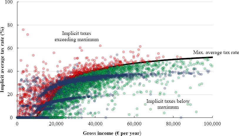
A first indication of the quality of individual gross and net incomes in SILC is provided by calculating implicit average tax rates, i.e. the difference between individuals’ observed gross and net income as a percentage of their gross income. Gross income is the sum of all market and non-market incomes before taxes and social assistance. Net income is the sum of gross income after social insurance contributions (excl. employer contributions) and personal income taxes. In Figure 1 we depict the distribution of these implicit tax rates at the individual level. We compute the maximum statutory average tax rate as the tax rate for an employee, depicted by the full black line. Note that this is an upper bound. For most tax payers, the implicit average tax rate is lower. All observations with implicit tax rates exceeding the statutory maximum are depicted in red, those below the upper bound are depicted in green. The blue dots represent the observations for which the statistical office imputed either the net or gross incomes, or both.

Implicit average tax rates (% of gross income).
Source: SILC 2010, authors’ own calculations.
The large variation in implicit tax rates is difficult to explain by the tax-benefit system itself. In fact, a large fraction of the observations are at odds with the actual tax rules: for 28.8% of the taxpayers the observed implicit tax rate exceeds the upper bound to what the tax rate can be for a person with his/her income. This implies that reported gross incomes are either too high or net incomes are too low, or both. As the Belgian tax system includes many tax reductions, it is much harder to conclude anything for implicit tax rates that are below the maximum average tax rate. Strikingly the implicit tax rates for observations with imputed incomes exceed the statutory maximum in many cases. Unfortunately we cannot assess the quality of the imputation process any further due to lack of information provided by the Statistical Office responsible for this imputation.
Table 1 shows the number of missing net and gross incomes as a share of the total number of observations per income type. Net incomes are reported much more often than gross incomes, as the fraction of observed values for net incomes is between 99.7% (unemployment benefits) and 77.3% (self-employment income). The fraction of observed values for gross incomes lies between 99.7% (unemployment benefits) and 37.8% (self-employment income). With the exception of gross unemployment benefits, gross incomes in SILC contain considerably more imputations than net incomes.
Imputations per income source.
| Number of observations | Number of imputed values | Imputed values as % of total | |||
|---|---|---|---|---|---|
| Income source | Net | Gross | Net | Gross | |
| Employment | 5,635 | 186 | 424 | 3.3 | 7.5 |
| Self-employment | 714 | 162 | 444 | 22.7 | 62.2 |
| Old age pensions | 2,423 | 331 | 1,165 | 13.7 | 48.1 |
| Survivor pensions | 103 | 7 | 37 | 6.8 | 35.9 |
| Unemployment benefit | 1,441 | 4 | 4 | 0.3 | 0.3 |
| Sickness benefit | 185 | 24 | 99 | 13.0 | 53.5 |
| Disability benefit | 471 | 17 | 202 | 3.6 | 42.9 |
-
Source: SILC 2010.
1.2 Matching SILC with IPCAL
The IPCAL database is an administrative dataset which contains the fiscal forms of the Belgian residents, with all variables relevant for the calculation of personal income taxes included. Within the FLEMOSI project1, we obtained an IPCAL dataset which contains the fiscal forms of the individuals included in the Belgian SILC 2010. This dataset was delivered with a unique identifier for each individual in both datasets, giving us the opportunity to perform a perfect one on one match of both datasets. They both contain information on incomes earned in 2009 (Decoster & De Swerdt., 2013).
Table 2 lists the number of observations that have (not) been matched. When calculating new SILC gross incomes (Section 5), we start from the EUROMOD2 base dataset of SILC, which contains information on 14,700 individuals, including children (first row in Table 2). Evidently, for most children we cannot find a corresponding tax return file as they are ‘fiscally dependent’ and have no income to declare. The p-file of SILC (second row in Table 2), which contains information for all individuals aged 16 or more, has 11,816 observations. Since these are all potential tax units, this is the relevant subpopulation to look for a corresponding record in IPCAL. The IPCAL dataset has 11,792 observations. Of the 11,816 individuals in the p-file of SILC, 11,656 observations have a corresponding record in the IPCAL data. This can be considered a very good match given that the p-file still contains fiscally dependent children. The remaining 136 observations in IPCAL, for which no corresponding record in the SILC could be identified, are discarded from any further analyses.
Number of matched observations.
| Dataset | Matched | Not Matched | Number of observations |
|---|---|---|---|
| EUROMOD | 11,656 | 3,044 | 14,700 |
| SILC (p-file) | 11,656 | 160 | 11,816 |
| IPCAL | 11,656 | 136 | 11,792 |
-
Source: SILC 2010 and IPCAL.
Given that 11,656 individuals of the EUROMOD base dataset have a corresponding tax return, 3,044 of a total of 14,700 SILC-individuals are either fiscally dependent or their tax-record is missing in the IPCAL dataset. 96% of these individuals are younger than 25. Hence, we can safely assume that the large majority of these individuals are ‘potentially fiscally dependent’ children. Summing the total number of tax returns, using the weights of the SILC data, we find that the total number of tax returns in the SILC and IPCAL datasets matches the official statistics on tax returns very well. For a total of 6.77 million tax returns, the SILC coverage is 96%, whereas the IPCAL coverage equals 99%.
2. Comparing gross incomes in IPCAL and SILC
Before comparing gross incomes in IPCAL and SILC, we make sure that the income concepts in both datasets are comparable. We then start the comparison, both at the household and individual level.
Total gross household income is captured in the SILC by one variable (HY010). Some adjustments are necessary to compare this variable with the IPCAL variable, as not all income components of HY010 are included in the income concept for tax purposes. Child allowances and social assistance, for example, are tax exempt. On the left hand side of Table 3, we list all the income components of HY010 that are included in the target income concept. On the right, the income types that are excluded are listed. Variable PY080, pension from private pension plans, is normally not included in HY010, but is included here because this information has to be declared on the tax form.
Components of household gross income (HY010) in SILC, included or excluded for comparison with taxable gross income in IPCAL.
| Included | Excluded | ||
|---|---|---|---|
| HY040G | income from rental of a property or land | HY050G | family/children related allowances |
| HY080G | regular inter-household cash transfer received | HY060G | social exclusion not elsewhere classified |
| HY090G | interests, dividends, profit from capital investment in unincorporated businesses | HY070G | housing allowances |
| HY110G | income received by people aged under 16 | PY021G | company car |
| PY010G | employee cash or near cash income | PY140G | education-related allowances |
| PY050G | cash benefits or losses from self-employment | ||
| PY090G | unemployment benefits | ||
| PY100G | old age benefits | ||
| PY110G | survivor benefits | ||
| PY120G | sickness benefits | ||
| PY130G | disability benefits | ||
| PY080G | pension from individual private plans |
It is possible, and even common, to have more than one fiscal unit in the same sociological household. In order to compare the same households in SILC and IPCAL, we aggregated all gross incomes on the level of the sociological household (as identified in SILC).
It is important to note that SILC and IPCAL report different gross income concepts: SILC reports gross income, whereas IPCAL reports gross taxable income (after social insurance contributions). In order to align both datasets, two options are possible: either calculate gross taxable income in SILC starting from gross income, or calculate gross incomes in IPCAL, starting from gross taxable income. We went for the latter option. We do this by applying an iterative procedure, as explained in Section 4.
2.1 Total household gross income
In this section we discuss the differences between gross incomes in IPCAL and SILC. The monetary differences presented in the tables are always the reported income from IPCAL minus the income from SILC. Amounts are annual and in Euro. Percentage differences are with respect to amounts in SILC (=((IPCAL–SILC)/SILC)*100). Thus, a positive (negative) monetary difference implies that the amount in the administrative data is larger (smaller) than in the SILC data. Similar for positive (negative) percentage differences. We mostly show the mean difference and the standard deviation of the differences, as well as a graphical summary of the dispersion of the differences.
Table 4 shows this information for total household gross income. Average gross household income in IPCAL amounts to €44,135 per year, compared to a lower €41,729 in SILC. Thus, on average, IPCAL gross income exceeds SILC gross income by on average 6%. Individual differences show a large dispersion: a standard deviation of more than €30,000. There are many households for which gross income in SILC is larger than in IPCAL. Since, on average, IPCAL gross income exceeds the SILC one, the positive differences outweigh the negative ones.
Total household gross income: IPCAL vs. SIL.
| Mean income | Mean difference IPCAL – SILC | Standard deviation | Number of observations | ||
|---|---|---|---|---|---|
| IPCAL (€/year) | SILC (€/year) | (€/year) | % | (€/year) | |
| 44,135 | 41,729 | 2,405 | 5.8 | 30,624 | 6,095 |
-
Source: SILC 2010 and IPCAL, authors’ own calculations.
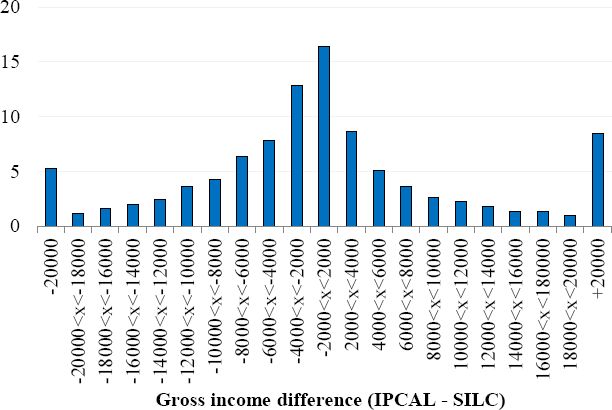
Figures 2 and 3 visualize the information on the two distributions in more detail. Figure 2 reveals that, for most lower and middle household gross incomes, frequency is lower in IPCAL than in SILC. The opposite can be said for higher gross incomes, mainly for the ones with a household gross income above 100,000 euro. The distribution of absolute differences (Figure 3) is quite symmetric. For large differences (a difference of more than €20,000), we have more positive ones (IPCAL exceeds SILC) than the reverse.
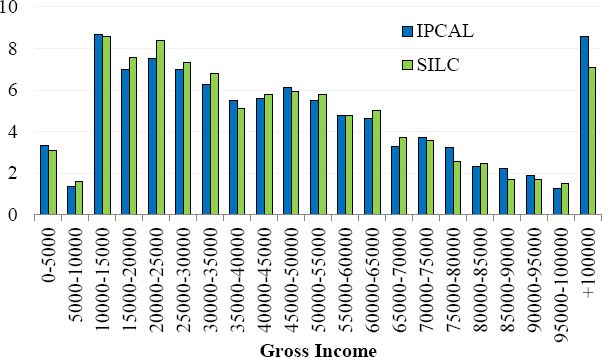
Distribution of total household gross income in IPCAL and SILC (% of observations).
Source: SILC 2010 and IPCAL, authors’ own calculations.

Distribution of differences in total household gross income in IPCAL and SILC (% of observations).
Source: SILC 2010 and IPCAL, authors’ own calculations.
The fact that total household gross income in SILC is, on average, lower than the one declared in the fiscal forms comes as a surprise to us. A priori, we would have thought that tax evasion and fraud, combined with trustful revelation in survey settings, would have led to the opposite result. It is of course possible that the administrative fiscal data contains incomes which are delayed and which should have been received in previous years but have actually been paid out in 2009, the year of the data collection. But, if they have actually been received in 2009, they should also be reported in the survey data as received in 2009. A preliminary conclusion is that some suspicion about the quality of gross incomes in SILC is warranted. This first finding calls for more detailed investigations. We start with analyzing the different income components separately.
2.2 Gross income components
We will only compare individuals who have a positive gross income component in both datasets. We first look at the correspondence between both datasets of the prevalence of income sources in Table 5.
Correspondence of gross income components in SILC and IPCAL (number and % of observations with positive income from income source).
| Number of observations | % of observations | ||||||
|---|---|---|---|---|---|---|---|
| Income source | IPCAL & SILC | IPCAL | SILC | Total | IPCAL & SILC | IPCAL | SILC |
| Employment (1) | 5,592 | 1,298 | 145 | 7,035 | 79.5 | 18.5 | 2.1 |
| Self-employment (2) | 567 | 218 | 307 | 1,092 | 51.9 | 20.0 | 28.1 |
| (1) and (2) | 6,187 | 1,049 | 146 | 7,382 | 83.8 | 14.2 | 2.0 |
| Old age pensions (3) | 2,291 | 298 | 122 | 2,711 | 84.5 | 11.0 | 4.5 |
| Survivor pensions (4) | 92 | 422 | 78 | 592 | 15.5 | 71.3 | 13.2 |
| (3) and (4) | 2,458 | 283 | 50 | 2,791 | 88.1 | 10.1 | 1.8 |
| Unemployment | 1,175 | 847 | 251 | 2,273 | 51.7 | 37.3 | 11.0 |
| Sickness (5) | 142 | 1,213 | 42 | 1,397 | 10.2 | 86.8 | 3.0 |
| Disability (6) | 65 | 498 | 402 | 965 | 6.7 | 51.6 | 41.7 |
| (5) and (6) | 503 | 881 | 136 | 1,520 | 33.1 | 58.0 | 8.9 |
| All | 9,476 | 777 | 164 | 10,417 | 91.0 | 7.5 | 1.6 |
-
Source: SILC 2010 and IPCAL, authors’ own calculations.
Almost 80% of all individuals recording a positive gross employee income in either IPCAL or SILC, report a positive income in both datasets. 18% have a positive employee income in IPCAL only. They often have small amounts of gross employee income (median of 2,237 euro and a mean of 13,100 euro, which points to a strongly right skewed distribution). It is possible that respondents in SILC forget about these small income amounts (e.g. because it is income from an occasional job). 2% have a positive income in SILC exclusively (median of 13,949 euro and a mean of 19,327 euro). Looking at self-employment income, the correspondence between both datasets is pretty low. 567 individuals have a self-employment income in both IPCAL and SILC, 218 in IPCAL only (a median of 3,733 euro and a mean of 8,040 euro) and 307 in SILC only (a median of 23,750 euro and a mean of 29,205 euro). The first mismatch may again be due to small amounts neglected by SILC respondents (an indication for this is the relatively low median income), while the second mismatch may be due to tax evasion (as median income is higher, this might be a plausible explanation). When taking both employee and self-employed gross income together (another possible mismatch is that people make wrong judgements whether they are working as employee or self-employed), we see that 84% of all individuals with work income report this income in both IPCAL and SILC. More than 1,000 individuals report a (relatively small) positive income in IPCAL but not in SILC (median of 1,606 euro and a mean of 5,623 euro).
For old-age pensions, the correspondence between both datasets is relatively good (85%). Again, we find that the median old-age incomes are low when the income component is present in IPCAL only (median of 2,052 euro with an average of 16,444 euro). When the old-age pension is reported in SILC exclusively, the median is higher (13,200 euro with an average of 14,271 euro). This underreporting of gross old-age pensions in IPCAL may be due to the fact that the amounts of the guaranteed income for the elderly are generally too low for taxes to be applied and are thus not declared to the tax authorities. For survivor pensions, the correspondence between both datasets is low (16%). Most individuals report a survivor pension in SILC but not in IPCAL. It is possible that individuals are not aware whether they receive an old-age pension or a survivor pension. When we take both income components together, the correspondence between both datasets is equal to 88%.
Looking at unemployment benefits, we once again notice a substantial mismatch between both datasets. Only 52% of all individuals with an unemployment benefit report this benefit in both datasets. 37% reports this benefit in IPCAL but not in SILC (median of 1,390 euro with an average of 3,083 euro), while the opposite is true for the remaining 11% (median of 2,669 euro with an average of 6,261 euro).
When looking at sickness and disability benefits, we see that the correspondence between both datasets is very low: only 10% for sickness benefits and 7% for disability benefits. For sickness benefits, most individuals (87%) report this (relatively low) benefit in IPCAL only and not in SILC (median of 2,469 euro and a mean of 5,166 euro). For disability benefits, the mismatch goes in both directions: 498 individuals report this benefit in IPCAL only and not in SILC, while the exact opposite is true for 402 individuals. When we take both sickness and disability benefits together (individuals may not know the difference between both benefits and report them incorrectly in SILC), we see that in only 33% of the cases the benefit is reported in both IPCAL and SILC.
Taking all previous individual gross income components together, we see that the correspondence for the actual reporting of a non-zero income between IPCAL and SILC is 91%. 7% report a (relatively low) gross income in IPCAL only (median of 1,677 euro and a mean of 6,486 euro), while 2% report a gross income in SILC exclusively (median of 13,200 euro and a mean of 18,033 euro). The first mismatch may be due to small amounts, neglected by the SILC respondents, while the second mismatch may be due to underreporting to the fiscal authorities.
In Table 6, we limit ourselves to individuals who report the same gross income component in both datasets. Looking at all income components together, the conclusion of the previous section is confirmed: in comparison to the administrative data, SILC underreports, on average, individual gross incomes. The average difference equals 3,930 euro per year or 15%.
Gross income components: IPCAL vs. SILC.
| Mean income | Mean difference IPCAL – SILC | Standard deviation | Number of observations | |||
|---|---|---|---|---|---|---|
| Income source | IPCAL (€/year) | SILC (€/year) | (€/year) | (% of SILC) | (€/year) | |
| Employment (1) | 33,455 | 31,554 | 1,901 | 6% | 8,736 | 5,592 |
| Self-employment (2) | 55,667 | 24,221 | 31,446 | 130% | 66,920 | 567 |
| (1) and (2) | 35,928 | 31,500 | 4,427 | 14% | 22,636 | 6,187 |
| Old age pensions (3) | 17,229 | 17,953 | −723 | −4% | 17,701 | 2,291 |
| Survivor pensions (4) | 14,839 | 13,883 | 955 | 7% | 2591 | 92 |
| (3) and (4) | 18,607 | 17,702 | 904 | 5% | 16,767 | 2,458 |
| Unemployment | 9,270 | 8,767 | 503 | 6% | 7,635 | 1,175 |
| Sickness (5) | 6,097 | 5,591 | 506 | 9% | 3,623 | 142 |
| Disability (6) | 3,907 | 11,914 | -8,007 | -67% | 7,988 | 65 |
| (5) and (6) | 10,608 | 9,932 | 676 | 7% | 5,986 | 503 |
| All | 30,462 | 26,533 | 3,930 | 15% | 23,852 | 9,476 |
-
Source: SILC 2010 and IPCAL, authors’ own calculations.
Zooming in on the different income components, we see that even for the well-defined and well-registered gross employee income component, the finding is persistent: gross employee income is lower in SILC than in IPCAL (average difference of 1,901 euro per year or 6%). Looking at gross self-employment income, the differences between SILC and IPCAL are enormous. On average, IPCAL income exceeds SILC income with more than 31,000 euro (or 130%) per year. In more than 60% of the cases whereby individuals report to have a self-employment income in both datasets, IPCAL income exceeds SILC income with more than 20,000 euro per year.
Old-age pension is an income component for which we find, on average, lower incomes in the fiscal data than in the survey data. Gross pension income as reported in SILC is, on average, 723 euro or 4% higher than in the IPCAL dataset. The opposite is true for survivor pensions, and for both pensions combined. We notice that the reported unemployment gross income is on average 503 euro’s per year higher in IPCAL than in SILC. In 13% of the cases, unemployment income in IPCAL is more than 20,000 euro’s per year higher as reported in SILC.
Finally, we find that sickness benefits in the fiscal data are higher than in the survey data (9%), while the opposite is true for disability benefits (difference of -67%). For both income components together we observe lower gross incomes in the survey data in comparison to the fiscal data.
2.3 Possible explanations for the underreporting of gross incomes in SILC
In this section, we focus on three elements which can (partly) explain the mismatch between gross incomes in SILC and IPCAL: (i) the imputation of missing values; (ii) the source of information used by the respondent; (iii) stability of the socio-economic status throughout the year.
First, we assess the role of the imputation process done by the Belgian Statistical Office. In Table 7, we look only at gross income components which are not imputed in the Belgian SILC dataset. As shown in Table 1, only unemployment benefits and employee incomes are captured relatively well, as most gross incomes are reported. For the other income components, considerably more values are imputed. Looking at total gross non-imputed individual income, we see that the mean difference between SILC and IPCAL goes down (from 15% to 12%). Also the standard deviation diminishes (from 23,852 to 22,336). Looking at the separate income components, we get a mixed picture: in all cases but one (old-age pensions), the mean difference between SILC and IPCAL diminishes. In some cases, the standard deviation decreases (employee income, unemployment income), while the opposite is true for self-employed income and old-age pensions.
Gross income components, not imputed: IPCAL vs. SILC.
| Mean income | Mean difference IPCAL – SILC | Standard deviation | Number of observations | |||
|---|---|---|---|---|---|---|
| Income source | IPCAL (€/year) | SILC (€/year) | (€/year) | (% of SILC) | (€/year) | |
| Employment (1) | 33,847 | 31,907 | 1,939 | 6% | 8,491 | 5,019 |
| Self-employment (2) | 63,761 | 27,777 | 35,984 | 130% | 93,942 | 134 |
| (1) and (2) | 34,296 | 31,390 | 2,906 | 9% | 18,281 | 5,390 |
| Old age pensions (3) | 17,395 | 18,370 | -974 | -5% | 19,944 | 1,195 |
| Survivor pensions (4) | 14,839 | 13,883 | 955 | 7% | 2,591 | 92 |
| (3) and (4) | 18,735 | 17,973 | 761 | 4% | 18,682 | 1,321 |
| Unemployment | 9,217 | 8,772 | 444 | 5% | 3,915 | 1,172 |
| Sickness (5) | 6,097 | 5,591 | 506 | 9% | 3623 | 142 |
| Disability (6) | 3,907 | 11,914 | −8,007 | −67% | 7988 | 65 |
| (5) and (6) | 10,608 | 9,932 | 676 | 7% | 5,986 | 503 |
| All | 30,812 | 27,473 | 3,339 | 12% | 22,336 | 7,513 |
-
Source: SILC 2010 and IPCAL, authors’ own calculations.
These findings indicate that an inaccurate imputation of gross income components partially explain the mismatch between gross incomes in IPCAL and SILC.
Next, we look at the information source used during the interview. In the Belgian version of the SILC, we have a variable indicating the source of information used by the respondents when filling in the questionnaire. We would expect that for respondents using either their tax or pay slip, SILC and IPCAL incomes should match rather well. Looking at Table 8, we see that this is indeed the case: both the mean difference between IPCAL and SILC (from 15% to 9%) and the standard deviation (from 23,852 to 16,421) diminishes. Zooming in on the different income components, we notice that the mean difference between IPCAL and SILC diminishes for some income components (e.g. self-employed income), while the opposite is true for others (e.g. unemployment benefit). The average standard deviation diminishes for all income components but one (old-age pension). Only a minority of the SILC respondents indicate to use extra information when filling in the questionnaire (39%). Problem groups are the self-employed (8.9%) and the pensioners (1.8%). Although the subgroup of self-employed persons who use extra sources is small (only 35 persons), the difference between their reported income in SILC and in IPCAL diminishes significantly (from 130% to -24%), indicating that using extra tax information systematically when filling in survey data may help reducing the mismatch with the fiscal data.
Gross income components, information used: IPCAL vs. SILC.
| Mean income | Mean difference IPCAL – SILC | Standard deviation | Number of observations | |||
|---|---|---|---|---|---|---|
| Income source | IPCAL (€/year) | SILC (€/year) | (€/year) | (% of SILC) | (€/year) | |
| Employment (1) | 36,293 | 33,991 | 2,302 | 7% | 8,218 | 3,480 |
| Self-employment (2) | 13,040 | 17,194 | −4,154 | −24% | 14,177 | 35 |
| (1) and (2) | 36,488 | 34,076 | 2,412 | 7% | 8,610 | 3,500 |
| Old age pensions (3) | 24,196 | 23,375 | 821 | 4% | 44,093 | 42 |
| Survivor pensions (4) | 15,426 | 13,788 | 1,638 | 12% | 1,871 | 6 |
| (3) and (4) | 23,097 | 21,791 | 1,306 | 6% | 39,898 | 51 |
| Unemployment | 5,731 | 4,926 | 805 | 16% | 4,433 | 268 |
| Sickness (5) | 4,799 | 4,098 | 701 | 17% | 3,111 | 63 |
| Disability (6) | 2,273 | 6,250 | −3,977 | −64% | 5,126 | 23 |
| (5) and (6) | 6,615 | 4,712 | 1,904 | 40% | 5,199 | 98 |
| All | 38,089 | 34,862 | 3,227 | 9% | 16,421 | 3,535 |
-
Source: SILC 2010 and IPCAL, authors’ own calculations.
As a final element, we look at individuals with the same socio-economic status throughout the year, as we could expect that these individuals have a better idea of their income in comparison to individuals who combine different income sources. Unfortunately, this element does not explain the mismatch between survey and fiscal data, as can be seen in Table 9. Both the mean difference between IPCAL and SILC and the standard deviation diminishes. But when we look at the different gross income components, we notice a better match between IPCAL and SILC data for some (e.g. pension or unemployment benefit), where the situation worsens for others (e.g. employment or sickness benefit). We can thus conclude that neither of the three elements discussed give a satisfying answer in explaining the mismatch between gross incomes in IPCAL and SILC.
Gross income components, same socio-economic status throughout the year: IPCAL vs. SILC.
| Mean income | Mean difference IPCAL – SILC | Standard deviation | Number of observations | |||
|---|---|---|---|---|---|---|
| Income source | IPCAL (€/year) | SILC (€/year) | (€/year) | (% of SILC) | (€/year) | |
| Employment (1) | 36,264 | 34,247 | 2,016 | 6% | 14,706 | 4,687 |
| Self-employment (2) | 63,873 | 38,533 | 25,340 | 66% | 73,582 | 325 |
| (1) and (2) | 38,765 | 33,905 | 4,860 | 14% | 23,947 | 5,250 |
| Old age pensions (3) | 17,257 | 17,740 | −483 | −3% | 13,470 | 2,209 |
| Survivor pensions (4) | 15,386 | 14,608 | 778 | 5% | 2,255 | 85 |
| (3) and (4) | 18,682 | 17,524 | 1,158 | 7% | 12,524 | 2,371 |
| Unemployment | 9,544 | 9,356 | 189 | 2% | 4,211 | 567 |
| Sickness (5) | 11,614 | 10,418 | 1,197 | 11% | 4,930 | 31 |
| Disability (6) | 5,216 | 16,065 | −10,850 | −68% | 8,358 | 41 |
| (5) and (6) | 12,942 | 12,472 | 470 | 4% | 6,750 | 343 |
| All | 31,390 | 27,417 | 3,973 | 14% | 22,093 | 8,486 |
-
Source: SILC 2010 and IPCAL, authors’ own calculations.
3. Constructing adjusted gross incomes
As none of the potential reasons assessed in Section 2.3 give a satisfactory explanation for the mismatch between the SILC and IPCAL gross incomes, we will explore one of several possible routes to adapt (or ‘adjust’) gross SILC incomes. The method we use is based on the assumption that SILC respondents have a better knowledge of their net incomes (as reported in SILC) than of their gross ones. The fact that gross incomes are more often imputed in SILC than net incomes (see Table 1) supports this argument. In this case, it seems naturel to start from the reported net incomes to reconstruct ‘corrected’ gross incomes, which are consistent with the reported net ones. Another option is to assume that the administrative gross incomes are the ‘correct’ ones, and hence replace (some) gross incomes in SILC by the information from IPCAL. A run of EUROMOD on these corrected gross incomes would then produce an adjusted net income distribution, which can be compared with the distribution of reported net incomes in SILC. We will only look at the former option, the latter is left for future research.
3.1 Methodology
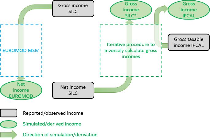
A microsimulation model (e.g. EUROMOD) establishes a relationship between gross and net incomes for a given tax-benefit structure. Immervoll and O’Donoghue (2001) invert this relationship by calculating gross incomes which correspond to given net ones. Since the complexity of a real-world tax-benefit system makes it impossible to invert this relationship analytically, one searches for these gross incomes iteratively. Make an informed guess of gross income, run the microsimulation model to calculate the corresponding net income, and compare this net income with the reported net income. Based on that difference, adjust the first guess of your gross income. In this way one produces a gross income distribution which, for a given tax benefit structure and for a given parameterization of this structure in a tax-benefit model, is consistent with observed or reported net incomes. In this case, the assumptions are: 1) that reported net incomes in SILC are more reliable than gross incomes, and 2) we take the accuracy of the microsimulation model, linking gross and net incomes, for granted. Figure 4 gives an illustration of the iterative procedure used in this paper.

Iterative procedure used to calculate new gross incomes in SILC.
The iterative method takes place in two steps. Starting from the reported net incomes, we first calculate the amount of taxes paid, hereby making use of the withholding income tax schedule as simulated within EUROMOD. We use the withholding income tax (and not the final income tax) because we expect that individuals in BE-SILC report their monthly net income equal to the monthly amount they receive on their bank account, which is gross income minus social security contributions minus withholding income taxes. We assume that a SILC respondent does not take into account the final tax settlement at the end of the fiscal year when reporting his or her monthly net income. In a second step, we use the sum of the net incomes and withholding taxes to estimate the amount of social security contributions paid. The ‘adjusted’ gross incomes are than the sum of originally reported net incomes, newly calculated withholding taxes and newly calculated social security contributions.
Below we compare the reported and adjusted gross income components in SILC, for each of the researched income components.
3.2 Gross employee income
In Table 10, we compare the adjusted gross incomes for employees (column 3) with the reported ones in SILC (column 2). We give both the absolute difference between adjusted and reported gross incomes (in euro per year) in column 4 and the percentage adjustment ((adjusted gross incomes – reported gross incomes) / reported gross incomes) in column 5. We do this by income deciles based on the equivalised net household income. In the two rightmost columns we sketch the progressivity of the implied tax rates, defined as the difference between gross incomes and net incomes as a percentage of gross incomes. Column 6 shows the implied tax rate when reported gross incomes are used. In column 7 we use the adjusted gross incomes.
Gross monthly income from employment, reported gross income vs. adjusted gross income, SILC 2010.
| (1) | (2) | (3) | (4) | (5) | (6) | (7) | |
|---|---|---|---|---|---|---|---|
| Decile | Income | Difference | Implicit tax rate | ||||
| reported net | reported gross | adjusted gross | (3)-(2)in € | (3)-(2) in % of (2) | (2)-(1) in % of (2) | (3)-(1) in % of (3) | |
| 1 | 3,288 | 4,296 | 3,456 | −840 | −19.6 | 23.5 | 4.9 |
| 2 | 10,356 | 13,632 | 12,012 | −1,620 | −11.9 | 24.0 | 13.8 |
| 3 | 14,628 | 20,460 | 19,248 | −1,212 | −5.9 | 28.5 | 24.0 |
| 4 | 17,268 | 24,720 | 24,204 | −516 | −2.1 | 30.1 | 28.7 |
| 5 | 19,224 | 28,116 | 28,908 | 792 | 2.8 | 31.6 | 33.5 |
| 6 | 21,048 | 30,876 | 32,796 | 1,920 | 6.2 | 31.8 | 35.8 |
| 7 | 23,064 | 34,548 | 37,512 | 2,964 | 8.6 | 33.2 | 38.5 |
| 8 | 25,500 | 39,180 | 43,044 | 3,894 | 9.9 | 34.9 | 40.8 |
| 9 | 29,208 | 46,176 | 51,792 | 5,616 | 12.2 | 36.7 | 43.6 |
| 10 | 42,696 | 68,676 | 87,504 | 18,828 | 27.4 | 37.8 | 51.2 |
| Total | 20,616 | 31,056 | 34,032 | 2,976 | 9.6 | 33.6 | 39.4 |
| Number of observations | 5,618 | ||||||
-
Source: SILC 2010, authors’ own calculations.
On average, gross monthly income from employment is adjusted upwards with nearly €3,000 or about 10%. But the adjustment varies widely across the income distribution. For the bottom four income deciles, gross employment incomes are adjusted downwards. For the upper half of the income distribution, we have to revise gross incomes upwards.
If we buy the assumption that SILC respondents report their net income more accurately than their gross income, and that they perceive the question as gauging their net earnings after withholding tax, this implies that respondents in the bottom deciles who also report a gross income, overestimate the withholding tax and social security contributions they have paid. On the contrary, individuals in higher deciles seem to underestimate the taxes and contributions paid. Since we have to revise their gross employment income upwards, the implied amount of taxes will, for a given net income, be higher.
The last two columns show how important the adjustment of gross incomes is when drawing conclusions about the progressivity of the tax system. Implicitly, accepting the correction of gross incomes as described above, and leaving the net incomes untouched, boils down to the introduction of a way more progressive tax system (in this case on employment income). The implicit tax rate in the top decile increases from 38% to 51%.
3.3 Gross self-employment income
Table 11 shows the adjustment for gross incomes from self-employment. Across the whole income distribution, we have to raise the gross incomes from self-employment to match the reported net incomes. In decile 10 we even have to add more than €52,000 or nearly 70%. In this case, it seems quite evident that the assumption of an accurate calculation of tax liabilities by EUROMOD is not really tenable. The upward adjustment of gross incomes will certainly also have to do with the fact that for self-employed, tax liabilities might be overestimated in EUROMOD.
Gross monthly income from self-employment, reported gross incomes vs. adjusted gross incomes, SILC 2010.
| (1) | (2) | (3) | (4) | (5) | (6) | (7) | |
|---|---|---|---|---|---|---|---|
| Decile | Income | Difference | Implicit tax rate | ||||
| reported net | reported gross | Adjusted gross | (3)-(2)in € | (3)-(2) in % of (2) | (2)-(1) in % of (2) | (3)-(1) in % of (3) | |
| 1 | 1,200 | 1,452 | 4,296 | 2,844 | 195.9 | 17.4 | 72.1 |
| 2 | 5,988 | 7,980 | 9,864 | 1,884 | 23.6 | 25.0 | 39.3 |
| 3 | 10,620 | 13,356 | 16,248 | 2,892 | 21.7 | 20.5 | 34.6 |
| 4 | 14,388 | 18,408 | 22,620 | 4,212 | 22.9 | 21.8 | 36.4 |
| 5 | 17,232 | 21,840 | 27,900 | 6,060 | 27.7 | 21.1 | 38.2 |
| 6 | 19,524 | 25,788 | 35,448 | 9,660 | 37.5 | 24.3 | 44.9 |
| 7 | 22,416 | 28,956 | 41,472 | 12,516 | 43.2 | 22.6 | 45.9 |
| 8 | 27,720 | 35,436 | 55,056 | 19,620 | 55.4 | 21.8 | 49.7 |
| 9 | 34,524 | 46,536 | 72,060 | 25,524 | 54.8 | 25.8 | 52.1 |
| 10 | 58,008 | 76,332 | 128,604 | 52,272 | 68.5 | 24.0 | 54.9 |
| Total | 20,436 | 26,544 | 39,576 | 13,032 | 49.1 | 23.0 | 48.4 |
| Number of observations | 700 | ||||||
-
Source: SILC 2010, authors’ own calculations.
3.4 Gross pension income
Looking at old-age pensions (Table 12), the adjusted gross incomes are lower in the bottom eight income deciles compared to the registered ones. This picture changes in the two highest deciles. The explanation for the low implicit tax rate in the bottom part of the distribution is twofold: old age pensioners are eligible for a substantial tax credits (2,202 euro per year in 2009) and they do not have to pay social insurance contributions if their monthly gross income is lower than 1,281 euro per month.
Gross monthly income from an old-age pension, reported gross incomes vs. adjusted gross incomes, SILC 2010.
| (1) | (2) | (3) | (4) | (5) | (6) | (7) | |
|---|---|---|---|---|---|---|---|
| Decile | Income | Difference | Implicit tax rate | ||||
| reported net | reported gross | adjusted gross | (3)-(2)in € | (3)-(2) in % of (2) | (2)-(1) in % of (2) | (3)-(1) in % of (3) | |
| 1 | 3,360 | 3,624 | 3,360 | −264 | −7.3 | 7.3 | 0.0 |
| 2 | 9,576 | 10,068 | 9,576 | −492 | −4.9 | 4.9 | 0.0 |
| 3 | 11,532 | 12,168 | 11,532 | −636 | −5.2 | 5.2 | 0.0 |
| 4 | 12,456 | 13,296 | 12,468 | −828 | −6.2 | 6.3 | 0.1 |
| 5 | 13,380 | 14,448 | 13,428 | −1,020 | −7.1 | 7.4 | 0.4 |
| 6 | 14,544 | 16,128 | 15,144 | −984 | −6.1 | 9.8 | 4.0 |
| 7 | 15,804 | 18,084 | 17,124 | −960 | −5.3 | 12.6 | 7.7 |
| 8 | 17,808 | 21,336 | 21,204 | −121 | −0.6 | 16.5 | 16.0 |
| 9 | 20,448 | 25,16 | 27,276 | 2,160 | 8.6 | 18.6 | 25.0 |
| 10 | 32,856 | 39,324 | 56,712 | 17,338 | 44.2 | 16.4 | 42.1 |
| Total | 15,108 | 17,256 | 18,684 | 1,428 | 8.3 | 12.4 | 19.1 |
| Number of observations | 2,423 | ||||||
-
Source: SILC 2010, authors’ own calculations.
Looking at survivor pensions (Table 13), adjusted gross incomes are on average lower than reported gross incomes in the first and second income tertile, and higher in the third income tertile.
Gross monthly income from a survivor pension, reported gross incomes vs. adjusted gross incomes, SILC 2010.
| (1) | (2) | (3) | (4) | (5) | (6) | (7) | |
|---|---|---|---|---|---|---|---|
| Tertile | Income | Difference | Implicit tax rate | ||||
| reported net | reported gross | adjusted gross | (3)-(2)in € | (3)-(2) in % of (2) | (2)-(1) in % of (2) | (3)-(1) in % of (3) | |
| 1 | 8,916 | 9,120 | 8,916 | −204 | −2.2 | 2.2 | 0.0 |
| 2 | 13,320 | 13,932 | 13,476 | −456 | −3.3 | 4.4 | 1.2 |
| 3 | 17,604 | 19,824 | 19,992 | 168 | 0.8 | 11.2 | 11.9 |
| Total | 13,188 | 14,196 | 14,028 | −168 | −1.2 | 7.1 | 6.0 |
| Number of observations | 103 | ||||||
-
Source: SILC 2010, authors’ own calculations.
3.5 Gross unemployment income, sickness and disability benefits
Newly calculated gross unemployment income (Table 14) is quite close to reported gross income (difference of 1.1% on average). The regressive pattern of taxation of unemployment benefits stays intact when calculating new gross unemployment incomes.
Gross monthly income from an unemployment benefit, reported gross incomes vs. adjusted gross incomes, SILC 2010.
| (1) | (2) | (3) | (4) | (5) | (6) | (7) | |
|---|---|---|---|---|---|---|---|
| Decile | Income | Difference | Implicit tax rate | ||||
| reported net | reported gross | adjusted gross | (3)-(2)in € | (3)-(2) in % of (2) | (2)-(1) in % of (2) | (3)-(1) in % of (3) | |
| 1 | 732 | 792 | 792 | 0 | 0.0 | 7.6 | 7.6 |
| 2 | 1,512 | 1,632 | 1,656 | 24 | 1.5 | 7.4 | 8.7 |
| 3 | 2,208 | 2,316 | 2,388 | 72 | 3.1 | 4.7 | 7.5 |
| 4 | 3,324 | 3,480 | 3,552 | 72 | 2.1 | 4.5 | 6.4 |
| 5 | 4,428 | 4,644 | 4,704 | 60 | 1.3 | 4.7 | 5.9 |
| 6 | 5,892 | 6036 | 6,264 | 228 | 3.8 | 2.4 | 5.9 |
| 7 | 8,436 | 8,748 | 8,772 | 24 | 0.3 | 3.6 | 3.8 |
| 8 | 10,392 | 10,584 | 10,716 | 132 | 1.2 | 1.8 | 3.0 |
| 9 | 11,556 | 11,748 | 11,724 | −24 | −0.2 | 1.6 | 1.4 |
| 10 | 15,516 | 15,756 | 15,996 | 240 | 1.5 | 1.5 | 3.0 |
| Total | 6,300 | 6,480 | 6,552 | 72 | 1.1 | 2.8 | 3.8 |
| Number of observations | 1,186 | ||||||
-
Source: SILC 2010, authors’ own calculations.
Individuals receiving a sickness benefit (Table 15) have to pay a withholding tax of 11.11% and also limited social security contributions. Adjusted gross incomes are about 10% higher than the net incomes in all income tertiles.
Gross monthly income from a sickness benefit, reported gross incomes vs. adjusted gross incomes, SILC 2010.
| (1) | (2) | (3) | (4) | (5) | (6) | (7) | |
|---|---|---|---|---|---|---|---|
| Tertile | Income | Difference | Implicit tax rate | ||||
| reported net | reported gross | adjusted gross | (3)-(2)in € | (3)-(2) in % of (2) | (2)-(1) in % of (2) | (3)-(1) in % of (3) | |
| 1 | 1,320 | 1,428 | 1,464 | 36 | 2.5 | 7.6 | 9.8 |
| 2 | 4,596 | 4,872 | 5,100 | 228 | 4.7 | 5.7 | 9.9 |
| 3 | 12,072 | 12,660 | 13,416 | 756 | 6.0 | 4.6 | 10.0 |
| Total | 5,952 | 6,276 | 6,612 | 336 | 5.4 | 5.2 | 10.0 |
| Number of observations | 182 | ||||||
-
Source: SILC 2010, authors’ own calculations.
Individuals receiving a disability benefit (PY140G) do not have to pay a withholding income tax or social security contributions (Table 16). Naturally, adjusted gross income (PY140G*) equals original net income (PY140N) in all income tertiles. The old gross incomes (PY140G) produced some strange implicit tax rates for which we found no explanation.
Gross monthly income from a disability benefit, reported gross incomes vs. adjusted gross incomes, SILC 2010.
| (1) | (2) | (3) | (4) | (5) | (6) | (7) | |
|---|---|---|---|---|---|---|---|
| Tertile | Income | Difference | Implicit tax rate | ||||
| reported net | reported gross | adjusted gross | (3)-(2)in € | (3)-(2) in % of (2) | (2)-(1) in % of (2) | (3)-(1) in % of (3) | |
| 1 | 168 | 600 | 168 | −432 | −72.0 | 72.0 | 0.0 |
| 2 | 480 | 732 | 480 | −252 | −34.4 | 34.4 | 0.0 |
| 3 | 2,100 | 276 | 2,100 | 1,824 | 660.9 | −660.9 | 0.0 |
| Total | 912 | 528 | 912 | 384 | 72.7 | −72.7 | 0.0 |
| Number of observations | 98 | ||||||
-
Source: SILC 2010, authors’ own calculations.
4. Comparing new gross incomes in SILC with IPCAL
In the final part of this paper, we compare the adjusted gross incomes in SILC with the IPCAL gross incomes and check whether using these new gross incomes improves the correspondence between both datasets. Reported gross incomes and newly calculated gross incomes are called “SILC reported” and “SILC adjusted” respectively.
4.1 Total household gross income
Like in Section 4, we show the differences between gross incomes in IPCAL and in SILC (either reported or adjusted), unless otherwise stated. Monetary differences are always the amount in IPCAL minus the amount in SILC. Amounts are annual and in euro. Percentage differences are with respect to the gross amounts in SILC (= ((IPCAL – SILC)/SILC)*100).
Table 17 gives information about the average difference in total gross household income between IPCAL and SILC (either reported or adjusted) for Belgium. Mean IPCAL gross household income exceeds mean SILC reported average income with 2,405 euro per year or 6%. Using new calculated gross SILC incomes, we see that the SILC incomes now exceed IPCAL gross household incomes with on average 1,821 euro per year or 4%. At first sight, new calculated gross SILC incomes perform better. Looking at individual differences, however, this picture changes: when we compare reported SILC gross household incomes with the administrative ones, we see a large dispersion with a standard deviation of more than €30,000. Using the new calculated gross SILC incomes, the standard deviation becomes even bigger: more than €42,000.
Total gross household income: IPCAL vs. SILC reported and SILC adjusted.
| Mean income | Mean difference IPCAL – SILC | Standard deviation | Number of observations | |||
|---|---|---|---|---|---|---|
| Income source | IPCAL (€/year) | SILC (€/year) | (€/year) | (% of SILC) | (€/year) | |
| SILC reported | 44,135 | 41,729 | 2,405 | 5.8% | 30,624 | 6,095 |
| SILC adjusted | 44,135 | 45,956 | −1,821 | −4.0% | 42,035 | 6,095 |
-
Source: SILC 2010, authors’ own calculations.
Figure 5 and 6 visualize the information on the three distributions in more detail. Figure 5 reveals that, for the lowest but mainly for the highest total gross household incomes (+€100,000), frequency is higher in SILC adjusted compared to IPCAL. In the middle categories, frequency is lower in SILC adjusted in comparison with SILC reported and IPCAL. Looking at the distribution of absolute differences (Figure 6), we see that for more than 15% of the cases, SILC adjusted gross income exceeds IPCAL income with more than 20,000 euro per year. In 8% of the cases, the opposite is true.

Distribution of household gross income in IPCAL, SILC reported and SILC adjusted (% of observations).
Source: SILC 2010 and IPCAL, authors’ own calculations.
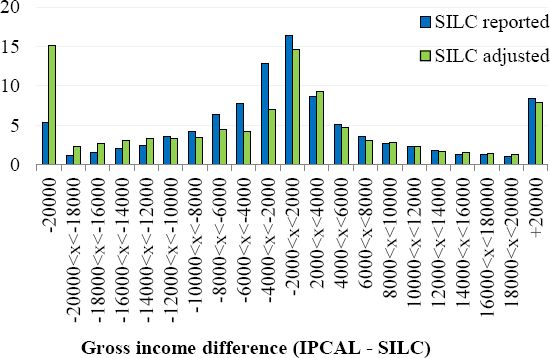

Distribution of differences in household gross income in IPCAL, SILC reported and SILC adjusted (% of observations).
Source: SILC 2010 and IPCAL, authors’ own calculations.
4.2 Gross income components
We now turn to an analysis of different income components at the individual level. We only compare individuals who have a positive gross income component in both IPCAL and SILC. On average, mean total gross individual incomes of IPCAL and SILC adjusted are now closer together (difference of 3%) than when we compared IPCAL with SILC reported data (difference of 15%). But the standard deviation is now higher (31,878 compared to 23,852).
Zooming in on the different income components (Table 18), we see that new calculated gross employee income is on average 1,067 euro higher in SILC. The percentage difference between IPCAL and SILC is now -3%, which is better than the average difference between IPCAL and reported SILC employee incomes (6%). But this comes at the cost of a higher standard deviation.
Gross income components: IPCAL vs. SILC adjusted.
| Mean income | Mean difference IPCAL – SILC | Standard deviation | Number of observations | |||
|---|---|---|---|---|---|---|
| Income source | IPCAL (€/year) | SILC (€/year) | (€/year) | (% of SILC) | (€/year) | |
| Employment (1) | 33,455 | 34,522 | −1,067 | −3% | 12,128 | 5,592 |
| Self-employment (2) | 55,667 | 34,797 | 20,870 | 60% | 68,014 | 567 |
| (1) and (2) | 35,928 | 35,694 | 234 | 1% | 25,306 | 6,187 |
| Old age pensions (3) | 17,229 | 19,722 | −2,493 | −13% | 42;037 | 2,291 |
| Survivor pensions (4) | 14,839 | 13,528 | 1,311 | 10% | 3,290 | 92 |
| (3) and (4) | 18,607 | 19,339 | −732 | −4% | 40,524 | 2,458 |
| Unemployment | 9,270 | 8,544 | 725 | 8% | 7,635 | 1,175 |
| Sickness (5) | 6,097 | 5,841 | 256 | 4% | 4,496 | 142 |
| Disability (6) | 3,907 | 3,622 | 285 | 8% | 1,582 | 65 |
| (5) and (6) | 10,608 | 9,969 | 639 | 6% | 4,178 | 503 |
| All | 30,462 | 29,673 | 789 | 3% | 31,878 | 9,476 |
-
Source: SILC 2010, authors’ own calculations.
Looking at self-employment income, there are still big differences between SILC and IPCAL. In more than 55% of the cases, IPCAL income exceeds both SILC reported and adjusted income with more than 20,000 euro per year. In 10% of the cases, adjusted SILC income is more than 20,000 euro per year higher than in the administrative counterpart. Once again, we can conclude that the SILC adjusted mean income is closer to the IPCAL mean, but this at the cost of a greater dispersion between the SILC adjusted data and the IPCAL data.
The results do not seem positive for the newly calculated gross pension incomes. The percentage mean difference between adjusted SILC and IPCAL is now −13% for old-age pensions and 10% for survivor pensions, which is higher than when using reported SILC data (respectively −4% and 7%). Also the standard deviation is higher for both old-age and survivor pensions.
The average difference between SILC and IPCAL incomes becomes bigger when using new calculated unemployment incomes in comparison to the reported ones. The standard deviation remains constant.
Finally, when looking at sickness and disability benefits, the average difference between SILC and IPCAL incomes diminishes when using the new calculated gross incomes. For sickness benefits, this comes at the cost of a higher standard deviation, where the standard deviation diminishes for disability benefits.
5. Conclusion
In this paper, we have tried to shed light on the quality of gross incomes as reported in the Belgian SILC. We did this for a unique sample of individuals for whom we had both administrative as well as survey data. For each of the individuals in the SILC data, information was requested from administrative tax data (IPCAL), resulting in a dataset with both survey and tax return data for the same individuals.
By calculating implicit tax rates, we got a first but not so reassuring indication of the quality of the gross incomes in SILC. Comparing SILC data with IPCAL data, we can conclude that gross incomes in administrative tax data are generally higher than in survey data and this holds true for most of the separate income components analyzed. These differences can be substantial, certainly for specific income components, such as self-employment income. We then tested some possible reasons for this underreporting of gross incomes in SILC (imputation in SILC, sources used by the SILC respondents and stability of the socio-economic status throughout the year), but none of them gave a satisfactory explanation.
To mitigate this ‘underreporting of gross incomes’ in SILC, we applied an iterative procedure for a net-to-gross imputation based on EUROMOD, assuming that net incomes reported in SILC are more accurate than gross incomes. Comparing the recalibrated gross incomes with the administrative IPCAL data yields mixed results. The differences in gross incomes that exist between survey data and administrative data do not become smaller.
Therefore, further analyses into the possible causes of these differences are certainly warranted. Since we do have an exact match between SILC and IPCAL information, we could replace SILC information on e.g. gross labour incomes by the IPCAL information. Another option is to insert additional information on fiscal expenditures into the EUROMOD dataset, as such produce a more accurate calculation of personal income tax liabilities. Since we then would have to expand EUROMOD with new information and also new routines, we leave this for future research. We consider this paper as a first step in a broader investigation of the quality of SILC gross incomes.
Footnotes
1.
FLEMOSI (Flemish Models of Simulation) was a SBO financed project of 4 years (2010–2014), in which five international partners joined forces to build a toolbox of state-of-the-art models to evaluate ex ante policy changes in Flanders. More information about the Flemosi project, the different models developed and the deliverables can be found at https://www.flemosi.be and in Decancq et al. (2012).
2.
EUROMOD is a tax-benefit microsimulation model for the European Union (EU) that enables researchers and policy analysts to calculate, in a comparable manner, the effects of taxes and benefits on household incomes and work incentives for the population of each country and for the EU as a whole. More information about EUROMOD can be found in Sutherland and Figari, 2013.
References
-
1
Estimating measurement error in annual job earnings: A comparison of survey and administrative dataReview of Economics and Statistics 95:1451–1467.
-
2
Mefisto: a new micro-simulation model for Flanders. Flemosi Discussion paper 14Mefisto: a new micro-simulation model for Flanders. Flemosi Discussion paper 14.
-
3
Fantasi: een microsimulatiemodel voor de personenbelasting op de IPCAL-data. Working Paper, Steunpunt Fiscaliteit en Begroting, Spoor A3b1Fantasi: een microsimulatiemodel voor de personenbelasting op de IPCAL-data. Working Paper, Steunpunt Fiscaliteit en Begroting, Spoor A3b1.
-
4
Challenges in income comparability. Experiences from the use of register data in the Norwegian EU-SILCPaper prepared for the VII International Meeting on Quantitative Methods of Applied Sciences.
-
5
Imputation of gross amounts from net incomes in household surveys. An application using EUROMOD. EUROMOD Working Paper no. EM1/01: EssexImputation of gross amounts from net incomes in household surveys. An application using EUROMOD. EUROMOD Working Paper no. EM1/01: Essex.
-
6
Measurement Error and Misclassification: a Comparison of Survey and Administrative DataJournal of Labor Economics 25:513–551.
-
7
Cross-validating administrative and survey datasets through microsimulationInternational Journal of Microsimulation 4:54–71.
-
8
Comparability of EU-SILC survey and register data: The relationship among employment, earnings and povertyJournal of European Social Policy 21:37–54.
- 9
-
10
EUROMOD: the European tax-benefit microsimulation model
Article and author information
Author details
Publication history
- Version of Record published: December 31, 2016 (version 1)
Copyright
© 2016, Vandelannoote et al.
This article is distributed under the terms of the Creative Commons Attribution License, which permits unrestricted use and redistribution provided that the original author and source are credited.