The Eurosystem household finance and consumption survey: A new underlying database for EUROMOD
- University of Antwerp, Belgium
- University of Insubria, ISER University of Essex, CeRP and DONDENA, Italy
- Article
- Figures and data
-
Jump to
- Abstract
- 1. Introduction
- 2. The opportunities of the HFCS data for microsimulation purposes
- 3. Constructing an HFCS database for Euromod
- 4. A pilot database for Belgium and Italy
- 5. Simulating net incomes using the HFCS data
- 6. The joint distribution of income and wealth
- 7. Conclusion
- Footnotes
- Annex
- References
- Article and author information
Abstract
We explore the prospects for using the Eurosystem Household Finance and Consumption Survey (HFCS) dataset as an underlying micro-database for the EU tax-benefit model, EUROMOD. This will allow expanding the policy domains currently covered in EUROMOD with dimensions like wealth taxation, incentives for wealth accumulation and asset tests determining benefit eligibility. As the HFCS only contains gross income amounts which are not suitable for distributive analysis, the purpose of this paper is to derive net incomes by simulating the gross-to-net transition with EUROMOD taking into account all important details of the social security and personal income tax system. In order to identify the issues and illustrate their importance a trial database for Belgium and Italy is constructed.
1. Introduction
Research on private wealth accumulation and concentration has recently received more prominence (see e.g. Jäntti, Sierminska, & Smeeding, 2008; Piketty & Saez, 2013; Piketty, 2014). Various publications have pointed towards increased income inequality over the past decades in many OECD (Organisation for Economic Co-operation and Development) countries, thdereby also devoting attention to the role played by wealth (see e.g. OECD, 2015). In this context the need for more comprehensive and integrated data on individual well-being is widely recognised, as for example highlighted in the Report by the Commission on the Measurement of Economic Performance and Social Progress (Stiglitz, Sen, & Fitoussi, 2009). For the component of wealth new household surveys as those developed as part of the Luxembourg Wealth Study (Jäntti, Sierminska, & Van Kerm, 2013) and the Eurosystem Household Finance and Consumption Network (HFCN) (HFCN, 2013a) represent a milestone in this ongoing process for better measurement. These databases can also be the corner stone for the analysis of policies that have been put forward as a way to reduce inequality, such as wealth and property taxation (e.g. Piketty, 2014). For this purpose it is important to assess the role of the different wealth components across countries, in order to set appropriate tax-free allowances and concentrate the tax burden on the wealthy part of the population, given the increasing role of housing assets in the household's portfolio along the entire income distribution (Figari, 2013). Furthermore, defining living standards in terms of income and wealth (e.g. Azpitarte, 2012; Brandolini, Magri, & Smeeding, 2010; Gornick, Sierminska, & Smeeding, 2009; Haveman & Wolff, 2004; Kuypers & Marx, 2016), opens up new perspectives on social policy. In light of current budgetary restrictions social benefits could be focussed on those who are most precarious, i.e. using the joint distribution of income and wealth as a means-testing tool (e.g. Menon, Perali, & Sierminska, 2016). Moreover, the framework allows for new policies to be introduced that focus on asset building among the poor (McKernan & Sherraden, 2008; Shapiro & Wolff, 2001; Sherraden, 1991).
This paper aims at contributing to assessing policy options in this area by exploring the prospects for using the HFCS dataset as an underlying database for a tax-benefit microsimulation model. The HFCS is a dataset covering detailed household wealth, gross income and consumption information (HFCN, 2013a), and thus provides more information on wealth than the current database underlying EUROMOD, which is the European Survey of Income and Living Conditions (EU-SILC), the standard database for poverty and inequality research in the European Union (EU). Both databases have their weaknesses and strengths and should be regarded as complements. Incorporating the HFCS data in EUROMOD will enhance empirical research possibilities in many ways. First, it will allow analysing the joint distribution of disposable income and net wealth based on information from the same survey, potentially comparable across countries and time. As the HFCS contains only gross income amounts which are not suitable for distributive analysis, we derive net incomes by simulating the gross-to-net transition with EUROMOD taking into account all important details of the social security and personal income tax system. Second, policy analysis will be enhanced in different ways, as the policy domains currently covered in EUROMOD will be expanded with dimensions like wealth taxation and asset building incentives, which recently gained much interest in the academic and the public debate. In addition, the model based on HFCS data would allow for an integrated assessment of taxable capacity taking into account direct taxes on income and wealth and tackling challenging issues such as those faced by ‘asset rich/income poor’ households (Hills, 2013). Moreover, it would enable to estimate the impact of reforms in wealth policies in interaction with other tax-benefit policies.
In order to identify the issues and illustrate their importance a trial database for Belgium and Italy is constructed. In the next section (Section 2) we argue why it would be interesting to integrate the HFCS database in a tax-benefit model like EUROMOD. In Section 3 we discuss the assumptions and transformations needed to construct a EUROMOD database on the basis of the HFCS data. Belgium and Italy are used as a case study (Section 4). Section 5 then studies the results of the derivation of net incomes for the HFCS data and validates them against those based on the current underlying database, EU-SILC. We provide some illustrative potential applications of the new tool in Section 6. The last section concludes (Section 7).
2. The opportunities of the HFCS data for microsimulation purposes
The main advantage of a tax-benefit microsimulation model is that it allows one to focus quite accurately on the objectives of social and economic policy, on the tools employed, and on the structural change experienced by those to whom the measures apply. Unlike a macroeconomic model, a microsimulation model allows one to simulate individual decision units. These decision units are typically households and the individuals that live in them. As described in Figari et al. (2015) different types of analysis are facilitated by using a microsimulation approach, among else the impact of tax-benefit policy changes (e.g. reforms regarding wealth and income taxation) on income-based indicators and related statistics and the impact of demographic factors on disposable income through the effects of tax-benefit policies (e.g. due to the presence of children). In order to exploit the cross-country dimension of the HFCS data, it is quite natural to build a database from the HFCS for EUROMOD, the EU-wide tax-benefit model, rather than for separate national tax-benefit models. EUROMOD simulates cash benefit entitlements and direct tax and social insurance contribution liabilities on the basis of the tax-benefit rules in place and information available in the underlying datasets for all EU countries. Instruments which are not simulated (mainly contributory pensions), as well as market income, are taken directly from the data (Sutherland & Figari, 2013). As such, EUROMOD is of value in terms of assessing the first order effects of tax-benefit policies and in understanding how policy reforms may affect income distribution, work incentives and government budgets in the short term. Moreover, EUROMOD is built in a way that maximises its flexibility and possibility to simulate tax-benefit policies on different databases.
Currently EUROMOD runs on the EU-SILC data, which has only limited information on wealth and income from wealth. The first purpose of running EUROMOD on the HFCS data is to derive a proper measure of disposable income, as the HFCS contains only gross income amounts which are not suitable for distributive analysis. This allows us to consider the joint distribution of disposable income and net wealth based on information coming from the same survey, potentially comparable across countries and time. Incorporating the HFCS data will allow expanding the policy domains currently covered in EUROMOD with dimensions like wealth taxation and asset building incentives; this is the second purpose of our study. This expansion will among others enable simulations relating to issues like a tax shift from income to wealth. It will help to understand and measure the redistributive role of these policies, also in relation to the other tax-benefit rules. Moreover, with subsequent waves of the HFCS coming available, the microsimulation model will also enable to investigate changes over time and to determine to what extent these are due to changes in the underlying population or to changes in the policies.
3. Constructing an HFCS database for Euromod
In order to be integrated in EUROMOD, a database needs to fulfil certain requirements, which are discussed in Section 3.1. Next, we show how the HFCS compares to the current EUROMOD database, namely EU-SILC, according to these requirements (Section 3.2). In Section 3.3 we provide an overview of the potential extension of the policy scope for EUROMOD.
3.1 What is needed for incorporating a new dataset in EUROMOD?
Figari et al. (2007) list a set of basic data requirements that a database must fulfil in order to be incorporated in a sensible way in EUROMOD.
Requirement a: The database used must be a recent, representative sample of households, large enough to support the analysis of small groups and with weights to apply to population level and to correct for non-response;
Requirement b: The database must contain information on primary gross incomes by source and at the individual level, with the reference period being relevant to the assessment periods for taxes and benefits. When benefits cannot be simulated, information on the amount of these benefits, gross of taxes, is required for each recipient;
Requirement c: The database must contain information about individual characteristics and within-household family relationships;
Requirement d: It must contain information on housing costs and other expenditures that may affect tax liabilities or benefit entitlements;
Requirement e: Specific other information on characteristics affecting tax liabilities or benefit entitlements (examples include weekly hours of work, disability status, civil servant status, private pension contributions) is also necessary;
Requirement f: The same reference period(s) should apply to personal characteristics (e.g. employment status) and income information (e.g. earnings) corresponding to it. In principle this implies the recording of status variables for each period within the year;
Requirement g: There should be no missing information from individual records or for individuals within households. Where imputations have been necessary, detailed information about how they were done is necessary.
In general, most of these requirements are met for the data we want to use, as is shown in the next section, where we make a comparison with the current EUROMOD input database, notably EU-SILC.
3.2 To what extent does HFCS fulfil the requirements?
The HFCS is a new dataset covering detailed household wealth, gross income and some consumption information (HFCN, 2013a). It is the result of a joint effort of all National Banks of the eurozone, three National Statistical Institutes1 and the European Central Bank (ECB). The first wave was made available to researchers in April 2013 and contains information on more than 62,000 households in 15 euro area member states which were surveyed mostly in 2010 and 20112. Ireland and Estonia are not included, but joined in the second wave (fieldwork period in 2014). Latvia, who joined the Euro zone on the 1st of January 2014, has also carried out the survey for the second wave.
The HFCS is a recent representative sample of households (see Section 3.2: Requirement a). For most countries, the sample size is large enough although it might not be exploited to conduct analysis on small groups in some countries (it might be too small for Slovenia with 340 households; in the other countries the sample size of the first wave ranges from 843 households in Malta to 15,006 in France). Survey weights take into account the units probability of selection, coverage issues, unit non-response and an adjustment of weights to external data (calibration) (HFCN, 2013a). An interesting feature of the HFCS dataset is that in most countries the very wealthy are oversampled such that a better coverage of the top of the income and wealth distributions is obtained. This is necessary because there exist large sampling and non-sampling errors as a consequence of the strong skewness of the wealth distribution. In particular the wealthiest households are less likely to respond and more likely to underreport, especially in the case of financial assets (Davies, Sandström, Shorrocks, & Wolff, 2011). Hence, in contrast to the EU-SILC sampling design which focuses on the households at the bottom of the income distribution, the HFCS focuses on the top (HFCN, 2013a, pp. 98–99). Since taxes typically have a larger impact on the top of the distribution the implementation of the HFCS in EUROMOD should lead to more accurate outcomes on the distributional and budgetary effects of taxation. The HFCN (2013b, p. 21) indicates that this oversampling strategy in some countries comes at the expense of coverage at the bottom of the distribution, but it is not clear to what extent this is the case in practice. Consequently, the benefit side of the redistributive system may still be better covered by EU-SILC.
The income components that are covered in the HFCS are largely the same as those surveyed in EU-SILC (see Section 3.2: Requirement b), be it that the HFCS data only covers gross income amounts which make them for instance unsuitable for the analysis of issues of inequality and redistribution. More specifically, the HFCS gross income concept includes the following components: employee income, self-employment income, rental income from real estate property, income from financial investments, income from pensions (public, occupational & private), regular social transfers, regular private transfers, income from private businesses and income from other sources (HFCN, 2013b, p. 108). The major differences with the income concept of EU-SILC are presented in Table 1. First, it is clear that in the category of employee income the HFCS only asks respondents about cash and near cash income, while EU-SILC also captures non-cash income. Secondly, pensions from mandatory employer-based schemes are included in public pensions in EU-SILC, while they are covered under private pensions in the HFCS (HFCN, 2013a, p. 100). Finally, income received by people under 16 is only covered in EU-SILC. In contrast, the HFCS covers income from other types of sources (such as capital gains or losses from the sale of assets, prize winnings, insurance settlements, severance payments, lump sum payments upon retirement), while EU-SILC does not.
Comparison of gross income components HFCS and EU-SILC.
| Category | HFCS | EU-SILC |
|---|---|---|
| Income from work | Cash & near cash employee income | Cash & near cash employee income |
| - - - | Non-cash employee income | |
| Self-employment income | Self-employment income | |
| Capital income | Rental income from real estate property | Rental income from real estate property |
| Income from financial investments | Aggregate variable including interests, dividends and profit from capital investments in unincorporated business | |
| Income from private business other than self-employment | ||
| Pension income | Aggregate variable of public pensions including old-age pensions, survivor pensions, disability pensions | Old-age benefits |
| Survivor benefits | ||
| Occupational & private pensions | Private pensions | |
| Social transfers | Unemployment benefits | Unemployment benefits |
| Aggregate variable of other social transfers including family/children related allowances, housing allowances, education allowances, minimum subsistence, other social benefits | Family/children related allowances | |
| Housing allowances | ||
| Education-related allowances | ||
| Sickness benefits | ||
| Social exclusion not elsewhere classified | ||
| Private transfers | Regular private transfers | Regular private transfers |
| Other income | - - - | Income received by people under 16 |
-
Source: HFCN (2013) & Eurostat (2014)
Similar to EU-SILC, the HFCS data contain information about individual characteristics and within-household family relationships (see Section 3.2: Requirement c). Also information on housing costs and other expenditures (see Section 3.2: Requirement d) and specific other information that may affect tax liabilities or benefit entitlements (see Section 3.2: Requirement e) are included in a similar way as is done in EU-SILC. The reference periods of the first HFCS wave range between 2008 and 2010; the income reference period generally refers to the year prior to that of the time of the survey, while the reference for the balance sheet (which includes wealth information) and the personal characteristics correspond in general to the time of the interview (see Section 3.2: Requirement f) (more details for Belgium and Italy are discussed further, indicating that there might be an issue).
Another interesting feature of the HFCS data is the use of a multiple imputation techniques to deal with selective item non-response (in the form of five different imputations) (see Section 3.2: Requirement g). Hence, crucial income and wealth information does not need to be imputed by researchers in the process of building the database. This imputation is not standardly performed in EU-SILC, implying that the researcher has to make decisions. Moreover, five different imputations will clearly lead to more accurate outcomes than a single imputation. The number of covariates used for the imputation, however, largely differs between countries as well as by income or asset type3. Moreover, the concrete variables that are used for these imputations are not documented. Therefore, the quality of imputations for individual countries may be hard to evaluate (Tiefensee & Grabka, 2014).
3.3 Enhancing the scope of policy analysis
The largest added value from using the HFCS data as an underlying database for EUROMOD is that it covers much more detailed information on wealth issues. This will allow the expansion of policy domains currently covered in EUROMOD with different types of wealth related policies: taxation of wealth and income from wealth, tax incentives for asset accumulation, asset means-testing in determining eligibility for social benefits, etc.
Table 2 provides an overview of the additional information available in the HFCS compared to EU-SILC regarding wealth; it also indicates a non-exhaustive list of extensions or refinements of the scope of policy analysis that follows from including the HFCS data in EUROMOD. The scope of analysis is clearly considerably enlarged when using the HFCS database, with e.g. taxes on different types of property, reliefs in the personal income tax for mortgage repayments and contributions to private pension funds, the value of social security wealth, adding wealth to the means-tests for eligibility of social benefits. There are, however, cross-country differences: for instance, the Italian dataset provides no information on the number of cars, on gifts and inheritances and the value of social security plans, occupational and voluntary pension schemes. As it is based on register information also the Finnish dataset lacks much information on these issues. Nevertheless, it is clear from Table 2 that the policy scope can be extended or refined substantially.
Comparison of available information in HFCS and EU-SILC.
| Belgium (2009) | Italy (2010) | ||||
|---|---|---|---|---|---|
| EUROMOD based on HFCS | EUROMOD based on EU-SILC | EUROMOD based on HFCS | EUROMOD based on EU-SILC | ||
| Main residence | Tax on property | ||||
| Size in square meters | Number of rooms | ||||
| Property value at time of acquisition, way and year of acquiring property, percent of ownership | - | ||||
| Self-assessed current price value | - | ||||
| Mortgages, up to 3: amount borrowed and still due, year and length of the loan, current interest rate, monthly amount of payment (capital + interests). More than 3: aggregate amount still due and monthly amount payment Missing: number of months paying capital + interests in a year | Annual amount of interests paid on mortgage(s) | Refinement of tax reliefs for mortgage interest repayments | |||
| Other real estate properties | Tax on property | ||||
| Up to 3: self-assessed current price value, property type, percent ownership More than 3: aggregate self-assessed current price value | - | ||||
| Mortgages, up to 3: amount borrowed and still owed, year and length of the loan, current interest rate, monthly amount of payment (capital + interests) More than 3: aggregate amount still due and monthly amount payment Missing: number of months paying capital + interests in a year | - | Tax reliefs for mortgage interest repayments | |||
| Cars | Tax on car property | ||||
| Number and value of cars and other vehicles | - | ||||
| Self-employment business | |||||
| Self-assessed value of the business, number of employees, NACE (Nomenclature statistique des Activités économiques dans la Communauté Européenne), legal form of the business | - | ||||
| Financial assets | Tax on financial assets | ||||
| Value of sight accounts, saving accounts, investments in mutual funds, bonds, shares, managed accounts, other financial assets | - | ||||
| Social security and pension assets | |||||
| Value of social security plans, occupational and voluntary pension schemes | - | Social security wealth | |||
| Contributions to private pension schemes | - | Refinement of tax reliefs for contributions to private pension schemes | |||
| Net wealth | Tax on net wealth, Net wealth means-test for eligibility of benefits | ||||
| All of the above | - | ||||
| Gift and inheritance | Tax on inheritance and gift | ||||
| Gift and inheritance received, number, year, kind of assets, value, from whom received | - | ||||
| Income from real estate property | Income from rental of a property or land | Tax on rental income | |||
| Income from financial assets | Refinement of tax on income from financial assets | ||||
| Income from deposits, mutual funds, bonds, non-self-employment private business, shares, managed accounts, other assets, voluntary pension/whole life insurance | Aggregate income from financial assets | ||||
-
Source: HFCN (2013a & b)
In the next section we turn to the construction of a trial database for two countries, notably Belgium and Italy, and highlight some specific issues related to this construction.
4. A pilot database for Belgium and Italy
In order to evaluate the suitability of the HFCS as a EUROMOD database we construct a trial dataset consisting of two countries (Belgium and Italy) and validate the main outcomes of running EUROMOD on the HFCS by comparing them with those obtained using EU-SILC as input database. The HFCS data potentially supply micro data on 15 euro area member states. However, the quality and reliability of the HFCS data is not clear yet for all countries. For Belgium an extensive validation of the HFCS data against external data sources such as EU-SILC and SHARE (Survey of Health, Ageing and Retirement in Europe) indicates that the HFCS is sufficiently reliable for the study of income and wealth in Belgium (Kuypers, Marx, & Verbist, 2015; see also Annex: Table A.1). The Italian HFCS survey was adapted from the prior existing Survey of Household Income and Wealth (SHIW) so that the strengths and weaknesses of these data are also relatively well-known (Ceriani, Fiorio, & Gigliarano, 2013)4. We make use of the UDB 1.1 data version of the HFCS (February 2015 release) on which we construct five new datasets where each of them contains information on one of the imputations. For our two countries we highlight practical issues of sample size, reference period, imputation of missing information, the disaggregation of certain variables into more detailed information, etc.
Sample
The UDB data for Belgium include information on 5,506 individuals living in 2,327 households. They were surveyed between April and October 2010, so that the reference income period is 2009. The oversampling of the wealthy was implemented based on the NUTS (Nomenclature of Territorial Units for Statistics) 1 region and the average income by neighbourhood of residence, which results in an effective oversampling rate of the top 10% equal to 47% (HFCN, 2013a). For Italy, the UDB data include 19,836 individuals from 7,951 households, with the fieldwork being done from January to August 2011; such that incomes refer to 2010. Contrary to practice in most other countries, no oversampling has been applied in Italy.
As mentioned before, missing information on crucial variables is multiply imputed, so that in principle the full sample can be used for the construction of the EUROMOD input database. Following common EUROMOD conventions, children that were born after the end of the income reference period are deleted from the sample in the EUROMOD input database5. In Belgium it concerns 18 children, and in Italy 100. Hence, as Table 3 shows the final sample covers 5,488 individuals for Belgium and 19,736 for Italy.
Descriptive statistics of sample and weights.
| Observations | Mean weight | Median weight | Min. weight | Max. weight | |
|---|---|---|---|---|---|
| Belgium | 5,488 | 1,961.1 | 1,274.8 | 149.7 | 12,205.7 |
| Italy | 19,736 | 3,032.6 | 1,826.8 | 3.04 | 22,802.1 |
-
Source: Own calculations based on HFCS.
Reference period
For Belgium, the HFCS questionnaire asks individuals to declare incomes received in 2009, but all aspects relating to assets and debt holdings as well as demographic and economic characteristics refer to the time of the interview. For Italy, the income reference period is 2010, while other aspects and characteristics relate to 31.12.2010. We have to make the assumption that these aspects have not changed compared to the income reference period. We deem it reasonable to assume that the largest share of individuals has not experienced a change in their main demographic and economic characteristics, or that such a change has no large impact on the outcomes. For countries where the crisis has led to large price fluctuations in housing or stock markets in these years, this assumption may affect outcomes, but this was not the case during the HFCS reference periods of Belgium and Italy (Sierminska & Medgyesi, 2013). In sum, the practice is basically the same as the one used when deriving an EU-SILC based EUROMOD input database.
Adjustments of variables
With the exception of certain variables, EUROMOD input variables on labour market information, incomes, benefits, etc. need to be covered at the individual level. As in EU-SILC a number of these components are surveyed at the household level in the HFCS. In order to divide these between individuals we followed the same process that was developed for the EU-SILC based input database. The components for which this applies are rental income from real estate property; income from financial investments; income from regular social and private transfers; and income from other sources6. Important to note is that the EUROMOD variable ‘INCOME: other’ in the EU-SILC refers to income received by individuals younger than 16 years, while it refers to income received from other sources in the HFCS (see Table 1).
Variables that could not be created using the HFCS as an underlying dataset and which are used in the Belgian EUROMOD simulations are firm size for the calculation of employer contributions and Belgian cadastral income of the main residence for the calculation of property taxes. For Italy cadastral income information is also missing. This implies that EUROMOD based on the HFCS slightly ‘undersimulates’ taxes and social contributions paid by households and hence slightly overestimates household disposable income.
Disaggregation of social transfers
In the original HFCS dataset all incomes from regular social transfers (except pensions and unemployment benefits) are covered under one aggregated variable, while EUROMOD requires all types of benefits to be covered separately. In case of Belgium this variable includes income sources received both at the individual (e.g. educational allowances) and the household level (e.g. housing allowances, family benefits, etc.). Child benefits and social assistance can be accurately simulated in EUROMOD and are considered to be the most important. Therefore, we opted to simulate the child benefit and social assistance in EUROMOD7, after which these two values are subtracted from the aggregate variable, resulting in a variable containing all other types of benefits. Where the simulated benefits turn out to be larger than the reported amounts, the residual benefits are set to zero when the difference is smaller than 150 euros per month, while for the households with dependent children we use the simulated child benefits on top of the reported benefits. Furthermore, the disaggregation of the overall HFCS public pension variable into EUROMOD input variables for old age, survivors and disability was imputed based on age, marital status and disability status.
Also for Italy, the HFCS dataset does not provide detailed information about specific benefits in distinct variables: in particular family allowances and unemployment benefits are provided together with employment income. Following Ceriani et al. (2013) we have not disaggregated the family allowances and unemployment benefits in separate variables due to the complexity of the rules but this choice was also justified by the fact that the validation on SHIW data found no overestimation of employment income (Ceriani et al. 2013).
Imputation of main residence mortgages
The HFCS dataset covers very detailed information on mortgages held for the main residence, among others the monthly payment that is made. However, the Belgian EUROMOD simulations require a specification of the part that is paid in interests and the capital part. We use the following formula to split the mortgage repayment into an interest and a capital part:
where i refers to the interest rate, n to the duration of the mortgage and k to the time of the mortgage period that already passed. Subtracting this interest part from the repayment amount gives the capital part. As wealth information in the HFCS refers to the time of the survey (2010 for Belgium), we assume that mortgage payments are the same in 2009 as in 2010. Mortgages that were taken or refinanced in 2010 are not included. We also assume all households to have made a payment during 12 months. This could be a problem if the mortgage was taken or has expired in the income reference period. Finally, we have to use information on the yearly interest rate applicable at the moment of the survey. Given that the first wave of the HFCS data refers to a crisis period, mortgages with adjustable interest rates might have rather large differences between 2009 and 20108.
Missing regional information
Unfortunately the HFCS UDB data do not include information on the region households live in. In the construction of the trial database we used for both countries a more or less representative region. Currently, this mainly affects the simulation of the additional regional surcharge to the personal income tax in both countries and the ‘Flemish Care Insurance Contribution’ in Belgium. In the case of Belgium we assumed all households to live in Flanders as this is the region with the largest population share; hence, the impact on our results should be as small as possible. In the case of Italy we simulated the additional regional surcharge based on the national tax rate (i.e. 1.23%) which is actually increased by the majority of regions resulting in an underestimation of the simulated total revenue. In the future this will be a much larger issue for Belgium as the sixth state reform of 2014 involves a substantial transfer of tax-benefit competences from the federal to the regional level.
5. Simulating net incomes using the HFCS data
In this section we discuss the outcomes from the EUROMOD process based on the HFCS data for Belgium and Italy, comparing the results with those obtained by the EU-SILC database. For the HFCS the reported figures refer to the mean over the five imputations. First, the comparison between EM-HFCS and EM-SILC of some socio-demographic characteristics of the weighted sample is presented in Annex: Tables A.1 and A.2. Overall, the composition is largely similar between HFCS and EU-SILC and also compared to the figures of the external source. For Belgium the HFCS appears to slightly overestimate the share of highly educated individuals. Since education is strongly correlated with income and wealth accumulation (Juster, Smith, & Stafford, 1999), this is likely due to the oversampling of the wealthy in the HFCS. Hence, the population weights do not seem to correct entirely for this overrepresentation in the sample. Furthermore, in the case of Belgium HFCS covers a lower share of outright home owners compared to EU-SILC, while the reverse is true with regard to the tenure status of Italian households.
All figures below are computed for individuals based on their household disposable income equivalised by the OECD modified scale9 and expressed in annual terms. Table 4 shows mean and median amounts of both original income and net disposable income calculated with EUROMOD (further abbreviated as EM; hence EM-HFCS refers to incomes simulated with EUROMOD based on HFCS and EM-SILC to those based on EU-SILC); the difference between them is the inclusion of taxes, social insurance contributions and benefits (including pensions).
Comparison of income inequality indicators between HFCS and EU-SILC.
| Belgium (2009) | Italy (2010) | |||
|---|---|---|---|---|
| EUROMOD based on HFCS | EUROMOD based on EU-SILC | EUROMOD based on HFCS | EUROMOD based on EU-SILC | |
| Original income | ||||
| Mean | 24,936 (654.6) | 1,500 (159.8) | 15,025 (116.1) | 15,937 (88.2) |
| Median | 17,904 | 19,755 | 11,820 | 12,568 |
| Gini coefficient | 0.57 (0.01) | 0.48 (0.003) | 0.52 (0.004) | 0.52 (0.002) |
| Disposable income | ||||
| Mean | 21,636 (311.3) | 20,177 (74.7) | 15,269 (75.9) | 16,906 (57.6) |
| Median | 18,847 | 19,067 | 13,235 | 14,899 |
| Gini coefficient | 0.32 (0.01) | 0.23(0.002) | 0.33 (0.003) | 0.33 (0.002) |
| Net wealth | ||||
| Mean | 336,068 (11,942.17) | 272,546 (5,834.23) | ||
| Median | 205,802 | 172,519 | ||
| Gini coefficient | 0.61 (0.01) | 0.61 (0.01) | ||
-
Source: Own calculations based on EM-HFCS and EM-SILC.
-
Notes: Original and disposable income are annual amounts equivalised using the modified OECD equivalence scale, all individuals considered. Wealth amounts are at household level, not equivalised. All figures are derived using sample weights. Standard errors are shown between parentheses.
In Italy, median and mean original income in HFCS are lower than those in EU-SILC. The HFCS median of original income in Belgium is found to be somewhat lower than the EU-SILC median (see also HFCN (2013a, p. 100) for a cross-country evidence), while mean estimates appear to be considerably higher based on the HFCS. The distributions of disposable income follow a similar pattern: median and mean income are lower in HFCS than in EU-SILC for Italy, while for Belgian disposable incomes, the medians are similar according to both datasets, while mean disposable incomes are higher according to HFCS. The comparison of the Gini coefficient shows very similar outcomes according to HFCS and EU-SILC for Italy. For Belgium, however, inequality indices are very different, with much higher inequality according to the HFCS data. This is probably due to the oversampling strategy applied in the HFCS for Belgium (and not for Italy, where the design of both surveys is very similar).
The bottom part of Table 4 presents some summary statistics on net wealth. We find that in Belgium mean net wealth is equal to about 336,000 euros, while the median reaches almost 206,000 euros. In case of Italy the amounts are 273,000 and 173,000 for the mean and median respectively. The Gini coefficients for both countries indicate that net wealth is much more unequally distributed than income.
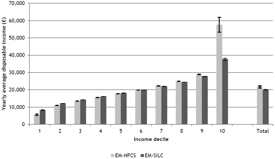
The large difference in Belgian Gini coefficients based on EU-SILC and HFCS suggests that it is not enough to look at median incomes (HFCN, 2013a, p. 100) to provide a reliable comparison between surveys. Therefore, Figure 1 shows average disposable incomes according to EM-HFCS and EM-SILC over income deciles for Belgium (see Annex: Table A.3 and Table A4 for Italy). It is clear that the difference in inequality is mainly driven by divergence at the top and the bottom of the income distribution. While the average equivalised disposable income in the 10th decile is equal to € 57,618 based on the HFCS, it is only € 37,832 for EU-SILC. The difference in average disposable income in the bottom decile is approximately 33% higher in EU-SILC than in the HFCS. Kuypers et al. (2015) show that despite their methodological similarities, distributional differences between HFCS and EU-SILC already exist at the gross income level. Moreover, differences are mainly found with regard to taxes and social insurance contributions, which are typically based on the income level, while outcomes for the benefits received are much more similar as eligibility is often based on non-monetary aspects such as the presence of children in order to qualify for child benefits. Hence, we attribute the difference in outcomes between the two surveys mainly to the HFCS oversampling strategy. Kennickell (2008) and Bover (2008) argue that on top of its correction for nonresponse, oversampling of the wealthy also provides more precise estimates of wealth in general and of narrowly held assets as standard errors are much smaller. Since oversampling in the Belgian HFCS data is based on average income by neighbourhood of residence (HFCN, 2013a), it also results in more accurate estimates of the top of the income distribution as well as of income sources that are typically received by a select group. Since what happens at the top of the distribution largely drives inequality trends (see Alvaredo, Atkinson, Piketty, & Saez, 2013; Piketty, 2014), we expect the HFCS to capture the level of inequality more closely to reality than EU-SILC. Vermeulen (2014), however, shows that despite the oversampling strategy wealth shares of the top 5% and 1% are still underestimated. It is not clear whether this is also the case for the income distribution. A comparison of HFCS and EU-SILC with official tax statistics (see Annex: Table A.5) suggests that EU-SILC underestimates the number of tax units and mean net taxable income at the top of the income distribution, while the HFCS appears to overestimate it.

Average disposable income by deciles according to EM-HFCS and EM-SILC, Belgium, 2009.
Source: Own calculations based on EM-HFCS and EM-SILC.
Notes: Decile groups based on disposable income equivalised using the modified OECD equivalence scale, all individuals considered. All figures are derived using sample weights.
6. The joint distribution of income and wealth
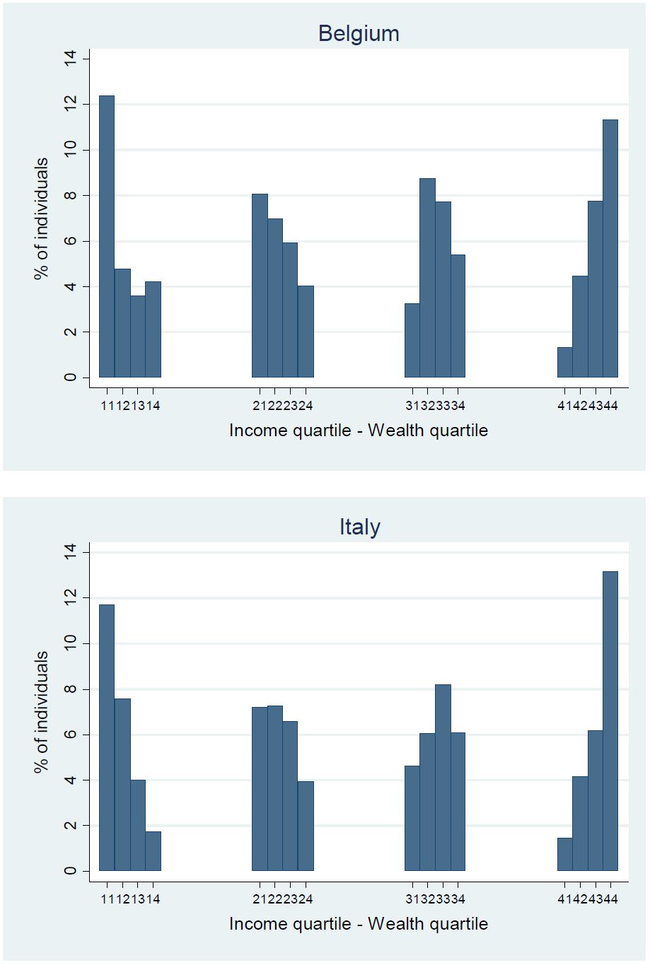
The availability of disposable incomes allows us to assess jointly the distribution of disposable income and net wealth for Belgium and Italy. We provide two illustrations of possible analyses. First, we consider the joint distribution of income and wealth according to quartiles. This may help to shed light to what extent income and wealth inequalities are jointly determined and interact with one another (see OECD (2015) for an example of the United States). Figure 2 shows the distribution according to income and wealth quartiles for the two countries. In the case of a perfect correlation, the options ‘11’, ‘22’, ‘33’ and ‘44’ should correspond to 25% each. This is, however, not the case, showing that there is considerable reranking of tax units if one would move from one distribution to the other. For instance, in both countries less than half of the tax units of the first income quartile are located in the bottom wealth quartile; a similar pattern is found for the top quartile. Nevertheless, the rank correlation between disposable income and net wealth at household level is positive (Spearman's rank correlation of 0.44 in Belgium and 0.62 in Italy), as one would expect given that higher wealth in general generates higher capital income. But given that the correlation is far from perfect, these outcomes illustrate that apart from income there are other drivers of wealth inequality that play an important role (e.g. gifts, inheritances, capital gains, etc.; see also Piketty, 2014).

Joint distribution of disposable income and net wealth, Belgium (2009) and Italy (2010).
Source: Own calculations based on EM-HFCS.
Notes: Quartile groups based on disposable income or net wealth equivalised using the modified OECD equivalence scale, all individuals considered. All figures are derived using sample weights.
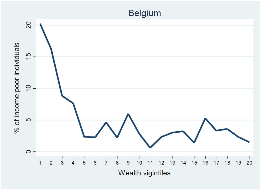
The newly developed database may also help to tackle challenging issues such as those faced by ‘asset rich/income poor’ households (Hills, 2013). Given that we have calculated disposable income, we are now able to identify income poor households and link this with their wealth situation. Figure 3 shows the share of those in income poverty (i.e. equivalent disposable income below 60% of the median) across the wealth distribution; we find that the highest share of poor people is found in the bottom of the wealth distribution. Nevertheless, income poor people are also found higher up the wealth distribution. For instance, in the top wealth quartile we find 16% of income poor people in Belgium, while it is 6% in Italy.

Distribution of income poor across wealth vigintiles, Belgium (2009) and Italy (2010).
Source: Own calculations based on EM-HFCS.
Notes: Vigintile groups based on net wealth equivalised using the modified OECD equivalence scale, all individuals considered. All figures are derived using sample weights.
These examples illustrate the complex interaction between income and wealth, which surely merits a more in-depth analysis.
7. Conclusion
Converting the HFCS data into an input database for EUROMOD creates many research opportunities. Our pilot exercise for Belgium and Italy indicates that it is feasible to use the HFCS database as EUROMOD input data, despite the fact that some of the outcomes need further investigation. Indeed, our results show that a comparison of results between EU-SILC and the HFCS cannot be based just on medians alone. It is important to look at the full distribution, as our outcomes show that there are some discrepancies at the bottom and especially at the top of the distribution. These discrepancies lead to important differences in the level of inequality in Belgium, which is assumed to be the consequence of the HFCS oversampling strategy. The oversampling of wealthy households might result in more accurate estimates of income and wealth at the top, although other potential reasons for the discrepancies should be investigated in more depth. These outcomes also provide an indication of the complementarity of both HFCS and EU-SILC; while EU-SILC is probably more suitable for research questions relating to the bottom of the income distribution, HFCS is probably more accurate for research focusing on the top. Nevertheless, a better understanding of the reasons of the discrepancies is something to be considered a priority for future research developments.
Footnotes
1.
Of France, Finland and Portugal
2.
Exceptions are France (2009/2010), Greece (2009) and Spain (2008/2009)
3.
For example, the imputation of missing values of employee income is based on 224 covariates in Spain, while the Netherlands use only 5 variables (HFCN, 2013a, p.51).
4.
Some other studies have looked at general aspects of data quality (e.g. Tiefensee & Grabka, 2014) or compared data sources for other countries (e.g. Westermeier & Grabka, 2015 comparing German HFCS with SOEP).
5.
In the HFCS we only know the age of the individual at the time of the interview, not the year in which they were born. We assume all individuals aged 0 years to be born after the income reference period.
6.
In practice this means that private and social transfers as well as other income are assigned to the household member whose age is closest to 45 years, while property and investment income are shared equally between the oldest household member and his/her partner. Hence, the assumption for the latter is that in the case of 3 generation households it is most likely that this kind of income is received by the oldest couple. This is in line with the life-cycle model of wealth accumulation (Ando & Modigliani, 1963).
7.
Similarly to the EU-SILC based simulations, the amounts of social assistance are adjusted for non-take-up of benefits with a random non take-up correction.
8.
Based on the HFCS data, in Belgium about 30 per cent of mortgages on the main residence have a variable interest rate, while this is about half in Italy.
9.
The OECD equivalence scale is constructed by giving the first adult a weight 1, any additional individuals aged 14 years or over 0.5, while individuals younger than 14 count for 0.3. As a sensitivity check we have also calculated outcomes with non-equivalised amounts, and the conclusions are broadly the same. 20112011201120112011
Annex
Comparison between EM-HFCS and EM-SILC of socio-demographic characteristics population, Belgium.
| EM-HFCS | EM-SILC | External Source* | ||
|---|---|---|---|---|
| Age | ||||
| < 16 | 17.7 | 18.2 | 18.1 | |
| 16–29 | 17.5 | 17.5 | 17.4 | |
| 30–44 | 21.3 | 21.0 | 20.5 | |
| 45–64 | 26.4 | 27.0 | 26.9 | |
| > 64 | 17.2 | 16.2 | 17.1 | |
| Gender | ||||
| Female | 51.0 | 50.8 | 50.9 | |
| Male | 49.0 | 49.2 | 49.1 | |
| Highest education achieved** | ||||
| Not completed primary | 12.8 | 18.2 | 15.9 | |
| Primary | 11.5 | 12.8 | 13.2 | |
| Lower secondary | 16.0 | 18.0 | 19.1 | |
| Upper secondary | 30.9 | 25.1 | 22.0 | |
| Post-secondary | 1.8 | 2.4 | ||
| Tertiary | 28.8 | 24.1 | 19.5 | |
| Labour market status | ||||
| Pre-school | 5.9 | 7.3 | 7.0 | |
| Employer or self-employed | 3.7 | 4.1 | 5.8 | |
| Employee | 36.3 | 35.7 | 36.9 | |
| Family worker | 0.1 | 0.2 | 0.7 | |
| Pensioner | 21.0 | 18.6 | 18.3 | |
| Unemployed | 6.5 | 5.1 | 3.6 | |
| Student | 19.8 | 18.1 | 17.6 | |
| Inactive | 0.0 | 1.4 | 1 | |
| Sick or disabled | 2.4 | 3.0 | 10.1 | |
| Other | 4.2 | 6.5 | ||
| Marital status | ||||
| Single | 46.6 | 44.7 | 45.6 | |
| Married | 40.8 | 40.5 | 40.2 | |
| Separated | N.A. | 0.3 | N.A. | |
| Divorced | 6.6 | 8.8 | 7.8 | |
| Widowed | 6.0 | 5.8 | 6.4 | |
| Tenure status | ||||
| Owner paying mortgage | 37.4 | 30.2 | 69.1 | |
| Outright owner | 36.2 | 41.6 | ||
| Tenant at market rate | 24.7 | 19.5 | 29.9 | |
| Tenant at reduced rate | 7.3 | |||
| 1.7 | 1.4 | 1.0 | ||
-
Source: Own calculations based on EM-HFCS and EM-SILC; External: CENSUS 2011 (Eurostat, 2016).
-
Notes: Statistically significant differences (at 5% level) are shown in italics;
-
*
Education and economic status of individuals aged below 15 imputed based on age;
-
**
Highest education achieved in external data unknown for 7.9%. All figures are derived using sample weights.
Comparison between EM-HFCS and EM-SILC of socio-demographic characteristics population, Italy.
| EM-HFCS | EM-SILC | External source* | |
|---|---|---|---|
| Age | |||
| < 16 | 15.1 | 15.0 | 14.9 |
| 16–29 | 15.2 | 14.9 | 14.5 |
| 30–44 | 21.8 | 23.2 | 22.1 |
| 45–64 | 27.5 | 26.7 | 27.6 |
| > 64 | 20.4 | 20.2 | 20.8 |
| Gender | |||
| Female | 51.6 | 51.4 | 51.6 |
| Male | 48.4 | 48.6 | 48.4 |
| Highest education achieved | |||
| Not completed primary | 9.6 | 13.7 | 14.2 |
| Primary | 21.4 | 19.3 | 19.7 |
| Lower secondary | 28.6 | 27.2 | 25.2 |
| Upper secondary | 30.9 | 30.1 | 28.0 |
| Post-secondary | 2.3 | ||
| Tertiary | 9.5 | 9.8 | 10.6 |
| Labour market status | |||
| Pre-school | 4.3 | 5.7 | 5.6 |
| Employer or self-employed | 7.5 | 8.4 | 8.1 |
| Employee | 30.5 | 29.2 | 32.8 |
| Family worker | 0.0 | 0.0 | 0.0 |
| Pensioner | 23.3 | 18.1 | 21.3 |
| Unemployed | 6.1 | 5.0 | 5.0 |
| Student | 17.7 | 15.7 | 14.7 |
| Inactive | 0.2 | 0.0 | 11.4 |
| Sick or disabled | 0.0 | 0.0 | |
| Other | 10.4 | 17.9 | |
| Marital status | |||
| Single | 38.1 | 40.3 | 41.2 |
| Married | 50.8 | 47.5 | 48.7 |
| Separated | N.A. | N.A. | N.A. |
| Divorced | 3.7 | 3.7 | 2.3 |
| Widowed | 7.5 | 8.5 | 7.8 |
| Tenure status | |||
| Owner paying mortgage | 11.6 | 15.4 | 73.0 |
| Outright owner | 58.1 | 56.5 | |
| Tenant at market rate | 20.5 | 18.8 | 17.9 |
| Tenant at reduced rate | |||
| Free user | 9.8 | 9.3 | 9.1 |
-
Source: Own calculations based on EM-HFCS and EM-SILC; External: CENSUS 2011 (Eurostat, 2016).
-
Notes: Statistically significant differences (at 5% level) are shown in italics;
-
*
Education and economic status of individuals aged below 15 imputed based on age. All figures are derived using sample weights.
Comparison between EM-HFCS and EM-SILC of means of different components by decile of equivalised disposable income, Belgium, 2009.
| Decile | Disposable income | Original income | Benefits | Taxes | Social insurance contributions |
|---|---|---|---|---|---|
| EUROMOD 2009 based on HFCS | |||||
| 1 | 5,559 | 1,526 | 4,217 | −19 | 203 |
| 2 | 10,971 | 5,009 | 6,606 | 127 | 516 |
| 3 | 13,526 | 7,982 | 7,117 | 657 | 916 |
| 4 | 15,540 | 11,741 | 6,911 | 1,609 | 1,503 |
| 5 | 17,693 | 15,297 | 7,245 | 2,894 | 1,954 |
| 6 | 19,796 | 19,579 | 6,870 | 4,001 | 2,652 |
| 7 | 22,192 | 25,034 | 6,287 | 5,816 | 3,312 |
| 8 | 24,850 | 30,455 | 6,189 | 7,678 | 4,115 |
| 9 | 28,904 | 38,049 | 6,984 | 10,944 | 5,186 |
| 10 | 57,618 | 95,212 | 8,249 | 36,142 | 9,732 |
| Total | 21,636 | 24,936 | 6,665 | 6,961 | 3,004 |
| EUROMOD 2009 based on EU-SILC | |||||
| 1 | 8,317 | 2,301 | 6,338 | −26 | 350 |
| 2 | 12,184 | 5,452 | 7,845 | 334 | 747 |
| 3 | 14,326 | 7,631 | 8,783 | 1,045 | 1,062 |
| 4 | 16,288 | 12,069 | 7,810 | 1,915 | 1,691 |
| 5 | 18,197 | 16,363 | 6,979 | 3,001 | 2,156 |
| 6 | 20,031 | 21,106 | 5,993 | 4,200 | 2,688 |
| 7 | 22,103 | 25,567 | 5,418 | 5,494 | 3,342 |
| 8 | 24,578 | 30,544 | 5,428 | 7,290 | 4,128 |
| 9 | 27,950 | 37,008 | 5,938 | 10,056 | 4,934 |
| 10 | 37,832 | 57,036 | 6,884 | 19,046 | 7,051 |
| Total | 20,177 | 21,500 | 6,741 | 5,233 | 2,832 |
-
Source: Own calculations based on EM-HFCS and EM-SILC.
-
Note: Annual income components equivalised using the modified OECD equivalence scale. All figures are derived using sample weights.
Comparison between EM-HFCS and EM-SILC of means of different components by decile of equivalised disposable income, Italy, 2010.
| Decile | Disposable income | Original income | Benefits | Taxes | Social insurance contributions |
|---|---|---|---|---|---|
| EUROMOD 2010 based on HFCS | |||||
| 1 | 3,779 | 2,904 | 1,349 | 132 | 341 |
| 2 | 7,371 | 5,629 | 3,011 | 687 | 583 |
| 3 | 8,957 | 6,498 | 4,277 | 1,183 | 635 |
| 4 | 10,392 | 7,126 | 5,600 | 1,623 | 711 |
| 5 | 12,217 | 10,075 | 5,357 | 2,208 | 1,007 |
| 6 | 14,162 | 13,013 | 5,182 | 2,718 | 1,314 |
| 7 | 16,213 | 15,305 | 5,808 | 3,365 | 1,535 |
| 8 | 18,836 | 19,617 | 5,532 | 4,378 | 1,936 |
| 9 | 22,802 | 24,641 | 6,444 | 5,791 | 2,492 |
| 10 | 38,108 | 45,609 | 9,124 | 11,829 | 4,795 |
| Total | 15,269 | 15,025 | 5,164 | 3,387 | 1,533 |
| EUROMOD 2010 based on EU-SILC | |||||
| 1 | 3,296 | 2,326 | 1,395 | 140 | 285 |
| 2 | 7,702 | 5,373 | 3,245 | 366 | 551 |
| 3 | 9,813 | 7,418 | 3,965 | 805 | 764 |
| 4 | 11,804 | 9,246 | 4,987 | 1,495 | 934 |
| 5 | 13,832 | 10,906 | 6,035 | 2,018 | 1,091 |
| 6 | 16,089 | 13,262 | 6,902 | 2,757 | 1,319 |
| 7 | 18,536 | 17,174 | 6,676 | 3,591 | 1,724 |
| 8 | 21,469 | 20,837 | 7,465 | 4,773 | 2,059 |
| 9 | 25,759 | 26,520 | 8,512 | 6,617 | 2,656 |
| 10 | 40,780 | 46,326 | 13,144 | 14,184 | 4,506 |
| Total | 16,906 | 15,937 | 6,232 | 3,674 | 1,589 |
-
Source: Own calculations based on EM-HFCS and EM-SILC.
-
Note: Annual income components equivalised using the modified OECD equivalence scale. All figures are derived using sample weights.
Comparison between tax statistics, EM-HFCS and EM-SILC of tax units and net taxable income, Belgium, 2009.
| Decile/Percentile | Tax statistics | EM-HFCS | EM-SILC | |
|---|---|---|---|---|
| Number of tax units | ||||
| 1 | 615,957.6 | 469,729 | 203,622 | |
| 2 | 615,957.6 | 550,059 | 523,956 | |
| 3 | 615,957.6 | 400,565 | 543,328 | |
| 4 | 615,957.6 | 535,845 | 544,909 | |
| 5 | 615,957.6 | 634,379 | 594,512 | |
| 6 | 615,957.6 | 460,388 | 556,651 | |
| 7 | 615,957.6 | 412,273 | 563,227 | |
| 8 | 615,957.6 | 499,893 | 624,264 | |
| 9 | 615,957.6 | 647,452 | 683,741 | |
| 10 | 615,957.6 | 711,359 | 552,271 | |
| 91 | 61,595.76 | 80,323 | 65,886 | |
| 92 | 61,595.76 | 81,886 | 65,088 | |
| 93 | 61,595.76 | 85,370 | 66,475 | |
| 94 | 61,595.76 | 63,196 | 52,019 | |
| 95 | 61,595.76 | 59,804 | 47,393 | |
| 96 | 61,595.76 | 36,264 | 54,328 | |
| 97 | 61,595.76 | 60,376 | 64,060 | |
| 98 | 61,595.76 | 45,649 | 55,509 | |
| 99 | 61,595.76 | 64,820 | 46,654 | |
| 100 | 61,595.76 | 133,671 | 34,859 | |
| Total | 6,159,576 | 5,078,337 | 5,286,509 | |
| Mean net taxable income | ||||
| 1 | 1,428 | 484 | 929 | |
| 2 | 8,632 | 8,633 | 8,944 | |
| 3 | 12,587 | 12,653 | 12,581 | |
| 4 | 15,427 | 15,465 | 15,466 | |
| 5 | 18,845 | 18,715 | 18,758 | |
| 6 | 22,639 | 22,740 | 22,691 | |
| 7 | 27,133 | 27,159 | 27,223 | |
| 8 | 33,982 | 34,265 | 33,962 | |
| 9 | 45,685 | 46,101 | 45,676 | |
| 10 | 87,118 | 111,794 | 79,162 | |
| 91 | 55,864 | 55,965 | 55,806 | |
| 92 | 58,508 | 58,459 | 58,570 | |
| 93 | 61,493 | 61,349 | 61,358 | |
| 94 | 64,904 | 64,836 | 64,810 | |
| 95 | 68,920 | 68,704 | 68,807 | |
| 96 | 73,909 | 73,258 | 73,970 | |
| 97 | 80,480 | 80,321 | 80,271 | |
| 98 | 90,005 | 89,502 | 89,312 | |
| 99 | 107,397 | 107,016 | 107,013 | |
| 100 | 209,700 | 286,309 | 183,816 | |
| Maximum | / | 2,348,883 | 727,625 | |
| Total | 27,339 | 35,175 | 29,412 | |
-
Source: Directorate-General Statistics, Department Economics of the Belgian Federal Government (2015) and own calculations based on EM-HFCS and EM-SILC.
References
-
1
The top 1 percent in international and historical perspectiveJournal of Economic Perspectives 27:3–20.
-
2
The 'life cycle' hypothesis of saving: Aggregate implications and testsAmerican Economic Review 53:55–84.
-
3
Measuring poverty using both income and wealth: A cross-country comparison between the U.S. and SpainReview of Income and Wealth 58:24–50.
-
4
Oversampling of the wealthy in the Spanish Survey of Household Finances (EFF)Irving Fisher Committee Bulletin 28:399–402.
-
5
Asset-based measurement of povertyJournal of Policy Analysis and Management 29:267–284.
-
6
The importance of choosing the data set for tax-benefit analysisInternational Journal of Microsimulation 6:86–121.
-
7
The level and distribution of global household wealthThe Economic Journal 121:223–254.
- 8
-
9
Working paper with the description of the ‘Income and Living Conditions dataset’Luxembourg: Eurostat.
- 10
-
11
The Eurosystem Household Finance and Consumption Survey - Methodological report for the first waveECB Statistics Paper, 1, 112.
-
12
The Eurosystem Household Finance and Consumption Survey - Results from the first waveECB Statistics Paper, 2, 112.
-
13
Should we make the richest pay to meet fiscal adjustment needs? - DiscussionThe role of tax policy in times of fiscal consolidation. European Economy, Economic Papers 502:103–107.
-
14
Using the EU-SILC for policy simulation: Prospects, some limitations and some suggestions. Comparative EU Statistics on Income and Living Conditions: Issues and challenges. Eurostat Methodologies and Working Papers, European Communities345–373, Using the EU-SILC for policy simulation: Prospects, some limitations and some suggestions. Comparative EU Statistics on Income and Living Conditions: Issues and challenges. Eurostat Methodologies and Working Papers, European Communities.
-
15
Microsimulation and policy analysisIn: AB Atkinson, F Bourguignon, editors. Handbook of Income Distribution Volume 2B. Amsterdam: Elsevier-North Holland. pp. 2141–2223.
-
16
The income and wealth packages of older women in cross-national perspectiveThe Journals of Gerontology Series B: Psychological Sciences and Social Sciences 64B:402–414.
-
17
The concept and measurement of asset poverty: Levels, trends and composition for the U.S., 1983–2001Journal of Economic Inequality 2:145–169.
-
18
Safeguarding social equity during fiscal consolidation: which tax bases to use? The role of tax policy in times of fiscal consolidationEuropean Economy, Economic Papers 502:80–91.
-
19
The joint distribution of household income and wealth. Evidence from the Luxembourg Wealth Study. OECD Social, Employment and Migration Working Papers No.65Paris: OECD Publishing.
-
20
The joint distribution of income and wealthIn: JC Gornick, M Jäntti, editors. Income inequality. Economic disparities and the middle class in affluent countries. Stanford: Stanford University Press. pp. 312–333.
- 21
-
22
The role of oversampling of the wealthy in the Survey of Consumer FinancesIrving Fisher Committee Bulletin 28:403–408.
-
23
Estimation of joint income-wealth poverty: A sensitivity analysisPaper presented at the 34th IARIW General Conference.
-
24
Joint patterns of income and wealth inequality in BelgiumReport prepared for the National Bank of Belgium.
- 25
-
26
An asset-based indicator of well-being for a unified means testing tool: Money metric or counting approach. LISER Working Paper No.2016-09.An asset-based indicator of well-being for a unified means testing tool: Money metric or counting approach. LISER Working Paper No.2016-09..
- 27
- 28
-
29
Top incomes and the Great Recession: Recent evolutions and policy implicationsIMF Economic Review 61:456–478.
-
30
Assets for the poor. The benefits of spreading asset ownershipNew York: Russell Sage Foundation.
-
31
Assets and the poor. A new American welfare policy. ArmonkNew York: M.E. Sharpe Inc.
-
32
The distribution of wealth between households. Social Situation Monitor European CommissionResearch note, 11/2013.
-
33
Report by the Commission on the Measurement of Economic Performance and Social ProgressReport by the Commission on the Measurement of Economic Performance and Social Progress.
-
34
EUROMOD: the European Union tax-benefit microsimulation modelInternational Journal of Microsimulation 6:4–26.
-
35
Comparing wealth - Data quality of the HFCS. DIW Berlin Discussion Paper No 1427.Comparing wealth - Data quality of the HFCS. DIW Berlin Discussion Paper No 1427..
-
36
How fat is the top tail of the wealth distribution? ECB Working Paper No. 1692.How fat is the top tail of the wealth distribution? ECB Working Paper No. 1692..
-
37
Significant statistical uncertainty over share of high net worth householdsDIW Economic Bulletin, 14/15.
Article and author information
Author details
Acknowledgements
This research was carried out as part of the research project “Matching, harmonization and integration of data suitable for the analysis of wealth taxation in the EUROMOD model” funded by the Joint Research Centre, IPTS, Knowledge for Growth Unit (Sevilla) of the European Commission (Tender JRC/SVQ/2015/J.2/0005/NC). We acknowledge the support and comments received by S. Barrios, F. Picos and M-L. Schmitz. We are indebted to all past and current members of the EUROMOD consortium. Sarah Kuypers and Gerlinde Verbist also acknowledge financial support from the Belgian Science Policy Office (BELSPO) under contract BR/121/A5/CRESUS. We thank the Editor, two anonymous referees and the participants at the HFCS Users’ Workshop (2015), Ecineq conference (2015) and IMA conference (2015) for helpful comments.
In this paper we make use of EUROMOD version G1.0 and microdata from the Eurosystem Household Finance and Consumption Survey (HFCS) and from the EU Statistics on Income and Living Conditions (EU-SILC). The results published and the related observations and analysis may not correspond to results or analysis of the data producers.
Publication history
- Version of Record published: December 31, 2016 (version 1)
Copyright
© 2016, Kuypers et al.
This article is distributed under the terms of the Creative Commons Attribution License, which permits unrestricted use and redistribution provided that the original author and source are credited.