Inequality and household size: A microsimulation for Uruguay
- Organismos Internacionales / Comisión Económica para América Latina y el Caribe, Uruguay
- Article
- Figures and data
- Jump to
Abstract
Declines in fertility and consequently in household size are among the main demographic changes that took place in many Latin American countries during the last decades. This demographic alteration may have had an impact on income distribution in case the patterns of decline were not similar between rich and poor households. In order to understand the driving forces of inequality changes in Uruguay, we consider the role of differential changes in reproductive behaviour and household formation on inequality and also on poverty, for two time periods (1996–2007 and 2007–2013). We estimate the effects of changes in the number of children in the household on mean income and specially, on the distribution of income and on poverty. Based on microsimulation techniques, our results indicate that both poverty and inequality would have been lower if changes in household size had not taken place among Uruguayan households. This ultimately implies that changes in fertility have contributed to higher levels of poverty and inequality, although the size of the total effect is not large. These results are mainly driven by a direct channel dominated by the evolution of the parameters that govern decisions about number of children in the household. Indirect effects, through the labour market, operated in a countervailing manner but due to their smaller magnitude, they were offset by the direct effect.
1. Introduction
Demographic factors are among the most important determinants of the evolution of income distribution and of its derived indicators such as poverty and inequality indexes. The relationship between inequality and demographic factors is a complex one, as many aspects – including household size and age composition – are involved. These elements are closely linked to fertility, whose differential patterns may be relevant. If fertility rates increase for the poor but decrease for the rich, this may affect income growth downwards in the short and medium run and have a considerable impact on inequality and poverty. This impact is exerted through a direct channel, as increasing the number of children in the household decreases per capita available income, or indirectly, as it may affect adults' decisions about labour market participation or hours of work. With a long run perspective, children from poorer households, which are more numerous, will accumulate less human capital and both income growth and its distribution will be affected (see for example De La Croix & Doepke, 2003). Given this, accounting for fertility differentials between the rich and the poor households is essential because it may have relevant consequences in the medium and long run. Moreover, if differential patterns of fertility have consequences on poverty and inequality, public policies affecting fertility may provide non expected gains in terms of poverty and inequality.
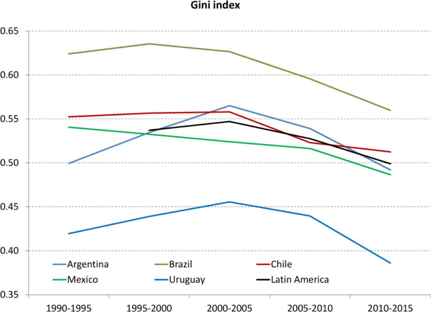
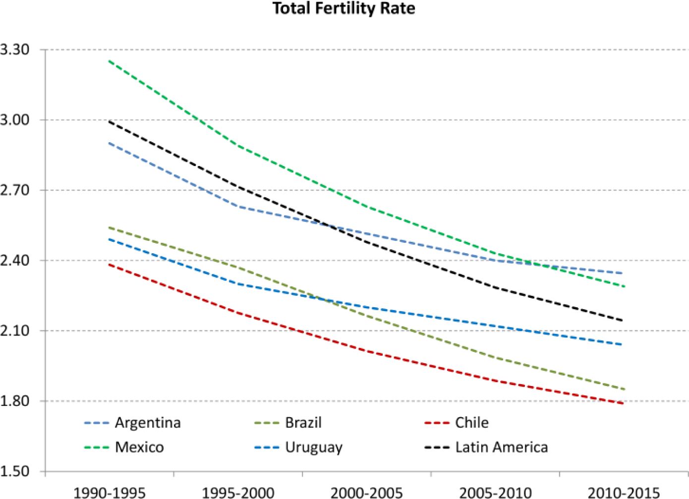
Concerns about the evolution of inequality in Latin America in recent decades have been in the core of academic discussion, as after the growing trend of the 90s, income inequality began to decrease in the 2000s, and the region made a strong progress towards reducing income disparities. The levels of fertility, on the other hand, have dropped significantly since the mid 50s. From 1990 on the trend decelerated but went on: total fertility rate went from 3 children per woman in 1990–1995 to the replacement level (2.1) by 2010–2015 (Figure 1.A in the Annex). These general trends in inequality and fertility are shared by many countries in the region, including Uruguay.
Income inequality and poverty increased between 1996 and 2004 in Uruguay, whereas household size, or more specifically the number of children per household, decreased on average, but its changes were not uniform along the income distribution. After 2004, poverty started to fall and from 2007 on, both income inequality and poverty decreased significantly, whereas the number of children per household continued its decreasing path. This article addresses the relationship between these three dimensions: poverty, inequality and the number of children per household, based on a microeconometric decomposition technique. A similar study for Argentina concluded that fertility decisions contributed considerably to changes in poverty and inequality in that country in the period 1980–1990 (Marchionni & Gasparini, 2007). Similar results are found by Badaracco (2014) for a set of Latin American countries, with the exception of Uruguay which shows a different pattern.1
In what follows, we focus on the relationship between changes in poverty and inequality and the dynamics of the number of children per household in Uruguay between 1996 and 2013, using a microeconomic perspective. The article is organized as follows: first we present some basic information about poverty, inequality and household size in Uruguay (Section 2). Then we outline the methodology of the microeconometric decompositions presented in the article (Section 3). Afterwards, we discuss the main results of our microsimulations (Section 4) and then present some final comments (Section 5).
2. Inequality, poverty and household size in Uruguay
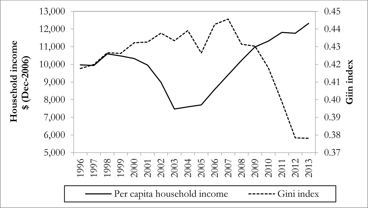
Uruguay is a small Latin American country, which stands out in the region for its relatively low levels of income inequality and poverty. It was classified as a middle income country until 2013, when it became high income for the first time. Average per capita household income increased in the beginning of the period and until 1999. After that, a period of recession began, and finished in the severe economic crises of 2002 and 2003. This recessive episode was due to a series of domestic and external shocks and implied an acute crisis of the financial system. In 2002 GDP (Gross Domestic Product) fell 11 % and the exchange rate slumped 90%. Household income, on the other hand, suffered a severe drop starting in 2000 (Figure 1). Between 2000 and the end of 2003, it decreased 28%. Although GDP began to recover in 2003, household income again decreased significantly that year (16%), and it only began to recover in 2004. Starting in 2006 household income climbed significantly, expanding almost 10% per year until 2009. From then on, with a brief interruption in 2012, household income grew at a more moderate rate of 4% annually. By the end of the period, household income reached and surpassed the pre-crises level.
In regard to income inequality, after remaining stable until the mid-nineties (Vigorito, 1999), all the inequality indexes showed an increasing trend during the recession and in the aftermath of the outbreak of the economic crisis in 2002. The Gini index for per capita household income, for example, was 0.42 in 1996 and rose to 0.44 in 2007 (Figure 1). From that year on, it has shown a sustained decrease, reaching its lowest figure in the last thirty years in 2013 at 0.38.
The increase in income inequality at the household level until 2006 comes from the labour market, as it is mainly explained by the increase in wage inequality. This is related to the fact that returns to skills increased significantly during the nineties. Different factors may have influenced the evolution of returns: openness, skill biased technological change, changes in wage bargaining, different evolution of real public transfers, among others (Bucheli & Furtado, 2005; PNUD, 2005). Other studies have underlined the importance of the suppression of centralized wage setting mechanisms, the drop in minimum wages and the lack of a social protection system oriented to the most deprived households as factors explaining the increase in inequality up to 2006 (Amarante et al., 2014). The relative importance of each factor as an explanation of the increase in inequality remains a matter of discussion. The decline in inequality after 2007 has also been related to different factors in the literature: the reduction in labour income inequality, the tax reform and the effect of noncontributory cash transfers (Amarante et al., 2014; Llambί et al., 2016), the significant increase in minimum wages (ECLAC, 2014) and the formalization in the labour market (Amarante et al., 2016). As in other countries in the region, the decline in the wage skill premium may have been related to the increase in the relative demand of unskilled workers, associated to commodity boom or related services (De la Torre & Pienknagura, 2012; Gasparini et al., 2012).

Household income and inequality.
Source: Own calculations based on household surveys.
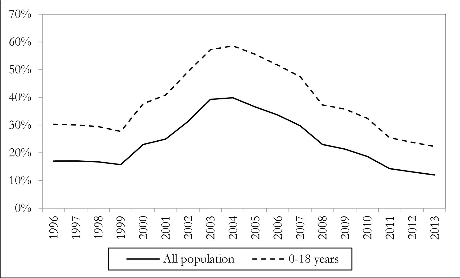
Poverty remained stable between 1996 and 1999 but amid a period of recession increased significantly during 1999–2002 (Figure 2).2 Furthermore, it continued on the upward trend in 2003 and 2004, standing at 30% on the latter year (more than doubling the figure of 1999). This increase is associated to the economic crises, which implied significant increases in the unemployment rate and reductions in real wages. In 2005, after three years of GDP recovery, poverty started to recede. This trend went on during the following years and towards the end of the studied period. In 2013, poverty stood at 12%, below pre-crisis levels and almost a third of the values registered just a decade ago. Some of the factors that explain the decrease in inequality also explain the decrease of poverty. In effect, non contributory cash transfers, increases in minimum wages and the increased demand of unskilled workers have translated into higher incomes at the bottom of the distribution, leading to lower poverty.

Poverty incidence. Uruguay. 1996–2013.
Source: Own calculations based on household surveys.
Poverty profiles about Uruguay always emphasize the differences of poverty incidence among age groups (Amarante et al., 2005; PNUD, 2005; World Bank, 2004). Child poverty was 22.3% in 2013, whereas poverty incidence among the whole population was 12.0%.2 This difference between child and adult poverty incidence is found for most Latin American countries, although the pattern is more acute in the case of Uruguay (see Rossel, 2013).
Consistently with these differences in poverty by age, there are significant differences in the number of children per household depending on the type of household and especially on the educational level of household head (Table 1)4. Besides differences in levels, the dynamics of the number of children per household were differential along the distribution. The number of children decreased during the last fifteen years in all households, no matter the educational level. Overall, it decreased almost 21%, changing from 1.66 to 1.32 (estimations based on households whose head is younger than 50). Nevertheless, the rates were differential according to the household head’s education, being higher the higher the level of education of the household head. Whereas the number of children decreased 6.2% for those households where the head had primary education or less, it decreased 33.6% when we consider households headed by persons with tertiary education (Table 1).
Number of children per household. Household head younger than 50.
| Number of children per household | Change | |||||
|---|---|---|---|---|---|---|
| Education (hh head) | 1996 | 2007 | 2013 | 1996–2007 | 2007–2013 | 1996–2013 |
| Primary or less | 1.97 | 2.03 | 1.85 | 3.0% | −8.9% | −6.2% |
| Secondary | 1.55 | 1.44 | 1.41 | −7.4% | −2.3% | −9.5% |
| Technical | 1.76 | 1.41 | 1.21 | −19.9% | −14.3% | −31.3% |
| Teachers | 1.32 | 0.98 | 1.01 | −25.5% | 2.7% | −23.4% |
| Tertiary | 1.26 | 0.90 | 0.83 | −28.4% | −7.4% | −33.6% |
| Total | 1.66 | 1.46 | 1.32 | −12.0% | −9.8% | −20.7% |
-
Source: Own calculations based on household surveys.
The analysis by income deciles shows a similar pattern: changes were differential by income deciles (Table 2). The mean average change in the number of children for households belonging to deciles 1 to 5 was −15% for the period 1996–2013, whereas the figure for deciles 6 to 10 was −33%.
Change in the number of children per household. Household head younger than 50.
| 1996 | 2007 | 2013 | 1996–2007 | 2007–2013 | 1996–2013 | |
|---|---|---|---|---|---|---|
| Deciles 1–5 | 2.23 | 2.11 | 1.91 | −5% | −10% | −15% |
| Deciles 6–10 | 1.09 | 0.82 | 0.73 | −25% | −11% | −33% |
| Total | 1.66 | 1.46 | 1.32 | −12% | −10% | −20% |
-
Source: Own calculations based on household surveys.
-
Note: Deciles are calculated on the basis of per capita household income.
3. Methodological aspects: microsimulation technique
Microsimulation techniques have emerged as useful instruments for economic analysis and policy recommendations. The well-known micro-econometric decompositions proposed by Oaxaca (1973) and Blinder (1973) for the study of the labour markets are early examples of the application of this technique. A generalized approach was developed by Bourguignon, Ferrerira, and Lustig (2004), and applied in Bourguignon, Forunier, and Gurgand (2001), among others. In this article, we use this method to assess the importance of the number of children per household on mean income, income distribution and poverty. Our analysis is based on household micro data for a specific Latin American country, Uruguay. Examples of micro-simulations for fertility decisions can be found in Ferreira and Leite (2002) and Marchionni and Gasparini (2007).
We take the adaptation of micro-simulation techniques proposed by Marchionni and Gasparini (2007) to analyse the role of fertility in Argentina. Following their proposal, (Dt) is per capita household income distribution corresponding to the (N) individuals in an economy in time (t:5)
where (yit) is the ratio between (Yh), total income of the household, and (Nh,) the family size
Family size is the sum of adults (Aht) and children (Chht) in the household:
Per capita household income of individual (i) is affected by fertility decisions in two ways: the increase in the number of children increases the denominator of the equation and, keeping other things constant, reduces per capita income for all household members. The number of children also affects the labour participation decision of some household members, modifying hours of work or the probability of participating in the labour market, and so affecting the numerator of the equation.
Total household income (Yht) is the sum of labour (L) and non labour incomes (NL) of all household members:
Non labour incomes are exogenously determined, whereas individual i’s labour income is the product of the hourly wage rate (w) and the number of hours of work (L).6
Labour market decisions can be modelled as originally proposed in Heckman (1974).7 Labour market reduced form equations are derived from a structural system obtained from a utility maximization problem of labour-consumption decisions. Wages (w*) are interpreted as marginal valuations of labour. They are a function of hours of work and other personal characteristics, and represent the minimum wage for which the individual would accept to work a certain number of hours. In equilibrium, if the individual decides to work, the number of hours devoted to labour should equate their marginal value (w*) with the wage received (w). If the marginal value is greater than the wage offered, given the individual’s characteristics, the person chooses not to work.
Then it is possible to model market determinants of wages offered (w) as a function of personal characteristics (standard Mincer equation). In equilibrium, the number of hours of work adjusts to make w=w*. Under general conditions, it is possible to derive a reduced form for the equilibrium relations in which wages and hours of work are expressed as functions of the exogenous variables. In this way, the model has two equations, one for wages (w*) and the other for hours of work (L*). These variables are functions of factors that affect wages (X1) and hours (X2), and that may or may not have elements in common. For our specific purposes, the number of children, (Ch), enters the labour supply equation. (ε1) and (ε2) represent unobservable factors that affect the determination of hours and wages respectively.
For estimation purposes, we observe positive values of (w*) and (L*) only for those individuals that actually work. So the reduced form model for wages and hours of work for individual (i) can be specified as:
With:
It can be assumed that:
The specification of labour market equations corresponds to the Tobit Type III model in Amemiya (1985). The parameters can be estimated through Heckman’s maximum likelihood method, using a censored version of (7) as selection equation, and estimating (6) using a Tobit model.
Fertility decisions, or more precisely the number of children in the household, are determined by some household observable characteristics (Zht), some unobservable characteristics (ε3ht), and the vector of parameters (ηt) that describe fertility decision:
In order to simulate the number of children in year (t) if the fertility parameter were that of (t’), we followed the strategy proposed in Marchionni and Gasparini (2007). Since the objective is to simulate changes in the number of children as a consequence only in the parameters of fertility, it is necessary to keep unobservable factors fixed. To do this, they characterize each household by the quantile it occupies in the distribution of children in year (t). The simulated number of children for each household will be the one that places it in the same quantile of the distribution of children with the relevant parameters of (t’), conditional on the observable characteristics in (t).
The combination of the above equations implies that household income depends on the following variables and parameters:
where X and Z may have variables in common.
The change of some of the parameters in this equation allows simulating incomes. In our case, we would like to simulate the number of children that household (h) in year (t) would have if fertility parameters were that of year (t’), that is .
Once the counterfactual number of children is estimated, per capita household income in equation (2) has to be recalculated, as the denominator changes. The change in income distribution resulting of this change in the number of children is called fertility-size effect. It reflects the contribution of the change in fertility parameters η to the change in income distribution through the direct channel, the change in the number of household members.
The second step consists on estimating the hours of work using the counterfactual number of children. With a different number of children, hours of work of individuals will change and this will imply different individual and household income. This implies computing the income that an individual of household (h) would have had at time (t) if the labour market participation decisions had changed in response to the number of children simulated using the fertility parameters of time (t), keeping all other things constant, even the number of people in the household. This simulated individual income allows to compute a simulated household income, and to compute the distributional impact of a change in the hours worked by individual (i) caused by a change in the number of children between years (t) and (t’). The family size in the denominator is kept constant. This effect is called the hours-size effect.
Marchionni and Gasparini (2007) propose a third simulation consisting of considering the counterfactual distribution in time (t) if parameter λ took the value estimated in year (t’). This parameter reflects the impact of a change in the number of children on individual’s hours of work. The distributional impact of changes in these parameters of the hours of work equation is named hours-parameter effect.
In order to perform the second and third micro-simulations, results on the simulated hours of work for all individuals, and their predicted wages, are needed. This implies having residuals for the hours of work and the wage equations for all individuals. These residual terms are not available for individuals who are not working at year (t). To obtain an estimation of residuals from both the hours of work and the wage equation, they were randomly sampled from the distribution of residuals (hours and wage) for working people at time (t). If the resulting prediction for year (t) is not consistent with the participation behaviour of the individual in year (t), these residuals were discarded. The process goes on until convergence was achieved.
Due to data availability, our main variable is the number of children per household instead of a direct indicator of fertility. The number of children is often used as a proxy for fertility in the economic literature (Klasen & Woltermann, 2005; Marchionni & Gasparini, 2007; among others). For biparental and lone households, the number of children acts as a very good proxy for fertility, although for extended households the relationship is not so close (see Amarante & Perazzo, 2011). Before going on, we should clarify some caveats of our methodology. It is basically a micro econometric decomposition, and so it is subject to the limitations often underlined in the literature, probably the most important being that only first order or partial equilibrium effects are considered. In our specific case, we capture first order impacts of demographic changes on income and its distribution. But these impacts on income could induce subsequent changes in fertility, which are not considered in our results. Moreover, demographic changes may have been induced by income modifications, and that is not captured by our model.
Our microsimulations are based on data from the Uruguayan household surveys (Encuesta Continua de Hogares) for 1996, 2007 and 2013. The survey is carried out by the Instituto Nacional de Estadistίca (INE) and covers the whole year, collecting detailed information about socioeconomic characteristics of households, income by sources and labour force attainment. The years considered in this study include a change in the coverage of the survey: up to 2005 the survey was restricted to urban centres of 5,000 inhabitants and more (85 per cent of the population), from 2006 on it has national coverage. Also, since 2006, the size of the survey was considerably expanded.8
4. Main results: the impacts of household size on inequality
In this section we present our main findings. First, we describe the main results related to the estimation of the fertility equation (4.1). In second place we describe results related to the estimation of labour market equations (4.2) and finally we present the results from micro-simulations (4.3).
4.1 The fertility equation
The first step of our modelization consists on estimating the number of children per household, Chi. This variable must be a non-negative integer and for this reason the use of count data models has been recommended in the literature, as they provide better specifications than linear models for demographic data (Melkersson & Rooth, 2000; Wang & Famoye, 1997; Winklemann & Zimmermann, 1994; among others). We consider Poisson and negative binomial models. Poisson distribution is based on the restrictive assumption of equi-dispersion, which may not be verified by data on completed fertility, whereas the negative binomial distribution is characterized by a greater variance than a Poisson with the same mean. Both models can be estimated by maximum likelihood (Greene, 2000).
Models were estimated using micro data for 1996, 2007 and 2013, considering households whose head was younger than 50. We considered three types of households: lone parents, bi-parental households and other households. One person households were excluded from the microsimulation, as they represent mainly elder people who had already finished their reproductive life. The fertility equation includes social and economic variables whose importance can be traced to the contributions of Becker (1960) about microfoundations of fertility decisions. These include opportunity costs given by parents’ earnings potential (reflected by their educational level and age), as well as controls for region and sex. Also, following cooperative bargaining models, variables reflecting unearned income were considered (see Chiappori, 1992; McElroy & Horney, 1981).
Results for households formed by couple and children are presented in Table 3. For these households, the negative binomial model converges to a Poisson in 1996 and 2013, but cannot be estimated in 2007. The number of children is decreasing with the level of education in the case of household head, reflecting higher cost of opportunity. Educational levels in our sample are categorized as low, medium and high. Low education comprises people who achieved as maximum educational level the primary school. Medium education refers to people who approved at least one year in secondary school (which in Uruguay starts in the seventh school year after kindergarten) and/or approved at least one year of technical education. High education is assigned to people who have approved at least one year in University, in any other tertiary education or in official school teaching academies. In all the years both medium and higher educated household heads tend to have fewer children than less educated.
In the case of the spouse (which are mainly women), both medium and higher educated also tend to have fewer children than less educated. It is also worth noting that coefficients are strictly decreasing with the level of education for both household heads and spouses. Moreover, the magnitudes of the coefficients for spouse’s education are higher than that of the household head, supporting Becker’s hypothesis of wife’s opportunity costs of having children.
Age of both the household head and the spouse show a significant and non-negative effect on fertility. Age squared is also significant but negative, indicating a non-linear, inverse U-shaped fertility-age profile. The coefficient on region is significant and negative reflecting lower number of children per household in the capital.9 Nevertheless the magnitude of this variable decreases throughout the years. The sex of the head of the household – categorized as 0 for men and as 1 for women- is significant and negative since 2007, although it is noted that bi-parental households headed by a woman are the minority. Nevertheless, this percentage has increased significantly, from 3% in 1996 to 12% in 2007 and 28% in 2013. Non labour income of the household head (in logs) is significant and positive for 1996, reflecting the wealth effect, although the magnitude is small. In 2007 non labour income of the household head is not significant and in 2013 it is significant and negative. Non labour income of the spouse is significant both years when data is available, yielding a small and unexpectedly positive sign.10
Results of the estimation of the fertility equations for other types of household are presented in Tables A.1 and A.2 (see annex). For lone parent households and other households fertility can be modelled through negative binomial models in every year, yielding similar results to Poisson. For these households, on the basis of the measure of goodness of fit based on the Akaike information criterion (Akaike, 1973), the Poisson model is preferred.
Estimation of fertility equations. Dependent variable: number of children in the household. Biparental households. 1996, 2007 and 2013.
| 1996 | 2007 | 2013 | ||||||
|---|---|---|---|---|---|---|---|---|
| OLS | Poisson | Neg. binomial | OLS | Poisson | OLS | Poisson | Neg. binomial | |
| Medium ed. Hh | −0.217 (0.0435)*** |
−0.116 (0.0251)*** |
−0.116 (0.0251)*** |
−0.404 (0.00632)*** |
−0.223 (0.0036)*** |
−0.301 (0.00562)*** |
−0.177 (0.00399)*** |
−0.145 (0.0097)*** |
| High educ hh | −0.242 (0.0672)*** |
−0.140 (0.0412)*** |
−0.140 (0.0412)*** |
−0.534 (0.00915)*** |
−0.324 (0.0624)*** |
−0.535 (0.00744)*** |
−0.365 (0.00580)*** |
−0.193 (0.00578)*** |
| Med. educ. sp. | −0.208 (0.0446)*** |
−0.109 (0.0255)*** |
−0.109 (0.0255)*** |
−0.38 (0.00653)*** |
−0.205 (0.00396)*** |
−0.287 (0.00574)*** |
−0.167 (0.00406)*** |
−0.135 (0.00403)*** |
| High educ sp. | −0.463 (0.0636)*** |
−0.260 (0.0393)*** |
−0.260 (0.0393)*** |
−0.653 (0.00866)*** |
−0.405 (0.00581)*** |
−0.495 (0.0037)*** |
−0.326 (0.00564)*** |
−0.188 (0.00563)*** |
| Age hh | 0.306 (0.0261)*** |
0.150 (0.0192)*** |
0.150 (0.0192)*** |
0.189 (0.00340)*** |
0.122 (0.00257)*** |
0.183 (0.00273)*** |
0.144 (0.00237)*** |
0.073 (0.00230)*** |
| Age2 hh | −0.004 (3.47e-4)*** |
−0.002 (2.53e-4)*** |
−0.002 (2.53e-4)*** |
−0.0025 (4.58e-5)*** |
−0.0016 (3.45e-5)*** |
−0.002 (3.70e-5)*** |
−0.002 (3.20e-5)*** |
−0.001 (3.10e-5)*** |
| Age spouse | 0.176 (0.0154)*** |
0.198 (0.0145)** |
0.198 (0.0145)*** |
0.19 (0.0225)*** |
0.169 (.00193)*** |
0.144 (0.00189)*** |
0.117 (0.00172)*** |
0.048 (0.00168)*** |
| Age2 spouse | −0.003 (1.95e-4)*** |
−0.003 (1.97e-4)*** |
−0.003 (1.97e-4)*** |
−0.0026 (2.9e-5)*** |
−0.0024 (2.6e-5)*** |
−0.002 (2.42e-5)*** |
−0.002 (2.26e-5)*** |
−0.001 (2.21e-5)*** |
| Region | −0.162 (0.0369)*** |
−0.087 (0.0219)*** |
−0.087 (0.0219)*** |
−0.148 (0.00502)*** |
−0.0898 (0.00334)*** |
−0.065 (0.00414)*** |
−0.046 (0.00321)*** |
−0.011 (0.00318)*** |
| Sex of hh | −0.110 (0.107) |
−0.102 (0.071) |
−0.102 (0.15) |
−0.095 (0.00777)*** |
−0.069 (0.00544)*** |
−0.013 (0.00504)** |
−0.007 (0.00396)* |
0.023 (0.00402)*** |
| Non lab inc hh | 0.011 (0.00200)*** |
0.006 (0.00115)*** |
0.006 (0.00115)*** |
0.0008 (0.000250)*** |
0.0003 (0.000166) |
−0.021 (0.000467)*** |
−0.012 (0.000315)*** |
−0.008 (0.000322)*** |
| Non lab inc sp | 0.010 (2.33e-3)*** |
0.005 (1.35e-3)*** |
0.005 (1.35e-3)*** |
0.003 (0.0002)*** |
0.0021 (0.00015)*** |
− (-) | − (-) | − (-) |
| Constant | −6.089 (0.424)*** |
−5.232 (0.314)*** |
−5.232 (0.314)*** |
−4.329 (0.0553)*** |
−4.242 (0.0433)*** |
−3.679 (0.0439)*** |
−3.908 (0.0400)*** |
−1.288 (0.0384)*** |
| Observations | 5,011 | 5,011 | 5,011 | 249,790 | 249,790 | 289,302 | 289,302 | 226,850 |
-
Standard errors in parentheses.
-
*
Significant at 10%;
-
**
significant at 5%;
-
***
significant at 1%.
-
Source: Own estimations based on household survey.
The estimations presented in this section confirm the results relative to the central role of education, and especially of spouse’s education, to determine the number of children.
4.2 Labour market equations
Two labour supply equations were estimated, one for hours of work and one for hourly wages. These equations were estimated separately for household heads and spouses (assuming that labour supply of the other members of the household does not depend on the presence of children), and for 1996, 2007 and 2013.
The labour supply equation is estimated using hours of work as the dependent variable, and including among the explanatory variables sex, age, age squared, a binary variable that indicates if the person lives in the capital of the country, a variable that reflects the number of children, a binary variable that indicates if the person is attending school, educational level (three levels: low, medium and high), a binary variable indicating if the person is married (or lives with her partner). For household heads, non-labour income was considered as an explanatory variable, whereas for spouses we included a variable reflecting income from the household head.
As discussed in the literature, some caveats may arise from the fact of the possible endogeneity of the number of children and hours of work. On this issue, Cruces and Galiani (2007) find no significant evidence of endogeneity of the number of children on their mothers’ labour participation decision. Based on that, Marchinnoni and Gasparini (2007) assume that the number of children is an exogenous variable in the labour market equations. This assumption was also taken in our case.
Results of the estimation using the Tobit method (maximum likelihood estimation) are presented in Table 4. Separate equations were estimated for household heads and spouses, for the years 1996, 2007 and 2013. In general terms, all coefficients yield the expected signs. In particular, hours of work are higher for men than for women. The relation between hours of work and age shows an inverse U pattern for the three years for spouses. For household heads the effect is likewise, though weaker. Living in the capital tends to be associated with higher hours of work in spouses, while recently household heads living in the rest of the country work more. The presence of children in the household has a negative impact on hours of work both for household heads and for spouses, but the magnitude of the effect is considerably higher for spouses, who are mainly women. A very relevant change has to do with the change in this coefficient for household heads. Whereas it was not significant in 1996, it turns significant and with an important effect in the other two years. In the case of spouses, the coefficients corresponding to the presence of children in the household are relatively stable in the period.
Both household heads and spouses who are attending school tend to work less hours per week. Hours of work increase with the level of education. The magnitude of the coefficient of these variables is considerably higher for spouses. The binary variable that distinguishes those who are married has a dual effect. On the one hand, is significant and positive for household heads in every year, while for spouses it is significant in 2007 and 2013, but negative, as expected according to traditional roles. In the case of household heads, higher non labour income is associated with lower hours of work in 1996 and higher hours of work in 2007 and 2013, although it is worth noting that the magnitude of the effect is quite narrow in all cases. In the case of spouses, higher income of the household head is clearly associated with lower hours of work, though the effect is diminishing throughout the studied period.
Labour supply. Dependent variable: hours of work. Tobit estimation.
| Household heads | Spouses | |||||
|---|---|---|---|---|---|---|
| 1996 | 2007 | 2013 | 1996 | 2007 | 2013 | |
| Sex | 7.31 (0.957)*** |
16.92 (0.0742)*** |
14.80 (0.0587)*** |
22.45 (2.829)*** |
25.22 (0.201)*** |
19.87 (0.111)*** |
| Age | 1.74 (0.322)*** |
1.66 (0.0397)*** |
2.21 (0.0335)*** |
4.71 (0.464)*** |
4.44 (0.0562)*** |
3.23 (0.0407)*** |
| Age | −0.02 squared (0.0044)*** | −0.02 (0.00054)*** |
−0.03 (0.00046)*** |
−0.06 (0.0063)*** |
−0.06 (0.00075)*** |
−0.04 (0.00054)*** |
| Region | 0.68 (0.527) |
−0.49 (0.0663)*** |
−1.02 (0.0578)*** |
4.03 (1.054)*** |
2.40 (0.127)*** |
1.10 (0.0941)*** |
| Children | −0.07 (0.196) |
−1.22 (0.0247)*** |
−0.97 (0.0237)*** |
−3.72 (0.405)*** |
−4.56 (0.0517)*** |
−3.75 (0.0416)*** |
| School | −10.83 (1.520)*** |
−7.33 (0.148)*** |
−3.48 (0.116)*** |
−4.36 (2.635)* |
−6.28 (0.263)*** |
−4.75 (0.185)*** |
| Med. educ. | 4.21 (0.586)*** |
5.29 (0.0801)*** |
5.72 (0.0762)*** |
14.71 (1.256)*** |
11.42 (0.169)*** |
8.02 (0.134)*** |
| High edu. | 6.71 (0.820)*** |
7.79 (0.108)*** |
6.89 (0.0952)*** |
29.21 (1.659)*** |
21.15 (0.214)*** |
14.52 (0.162)*** |
| Married | 3.77 (0.899)*** |
1.51 (0.0701)*** |
0.56 (0.0626)*** |
29.50 (19.16) |
−0.79 (0.141)*** |
−0.95 (0.101)*** |
| Non lab inc. | −0.39 -0.39 (0.0306)*** |
0.36 (0.00375)*** |
0.33 (0.00559)*** |
|||
| Income of hh. | −3.86 (0.731)*** |
−1.57 (0.0754)*** |
−0.60 (0.0628)*** | |||
| Constant | −3.17 (5.693) |
−5.21 (0.696)*** |
−17.00 (0.585)*** |
−85.33 (21.34)*** |
−57.53 (1.13)*** |
−37.34 (0.905)*** |
| Observat-ions | 7,648 | 405,657 | 463,118 | 5,448 | 258,113 | 285,446 |
-
Standard errors in parentheses.
-
*
Significant at 10%.
-
**
significant at 5%.
-
***
significant at 1%.
-
Source: Own estimations based on household surveys.
The estimation of the wage equation was undertaken using Heckman’s proposal. A censored version of the labour supply equation was used as the selection equation. The wage equation was estimated separately for household heads and spouses, considering all households included for the fertility equation estimation. The estimation was done using maximum likelihood. Hourly wages, in logs, is the dependent variable, and the independent variables are sex, age, age squared, region, three binary variables that indicate educational level (low, medium and high), and a binary variable indicating if the person is married or not. The selection equation includes all the variables included in the labour supply equation. So it adds as selection the number of children, a binary variable that indicates if the person is attending school, and a variable that reflects non labour income (in logs) for household heads, or the income of the household head (in logs) for spouses.
Results for the three years considered are presented in Table 5 for household heads and in Table 6 for spouses. Wages are higher for men, and present the expected inverse U pattern in relation to age. Wages are higher in Montevideo (where region equals one) and, as expected, wages are increasing with the level of education. Interestingly, the regional difference tends to vanish by the end of the period.
Wage equation estimation with selection correction (Heckman maximum likelihood). Dependent variable: hourly wages. Household heads.
| 1996 | 2007 | 2013 | ||||
|---|---|---|---|---|---|---|
| Hourly wages | Selec. eq. | Hourly wages | Selec. eq. | Hourly wages | Selec. eq. | |
| Sex | 0.191 (0.031)*** |
0.155 (0.072)** |
0.126 (0.0034)*** |
0.939 (0.0066)*** |
0.098 (0.0023)*** |
0.881 (0.0059)*** |
| Age | 0.068 (0.010)*** |
0.090 (0.024)*** |
0.021 (0.0015)*** |
0.139 (0.0035)*** |
0.032 (0.0013)*** |
0.154 (0.0029)*** |
| Age sq. | −0.0008 (1.4e-4)*** |
−0.0012 (3.3e-4)*** |
0.0000 (2.1e-5)** |
−0.0018 (4.8e-5)*** |
−0.0003 (1.8e-5)*** |
−0.0020 (4.1e-05)*** |
| Region | 0.299 (0.017)*** |
0.005 (0.042) |
0.146 (0.0025)*** |
0.045 (0.0065)*** |
0.062 (0.0022)*** |
−0.092 (0.0056)*** |
| Med. educ. | 0.338 (0.019)*** |
0.275 (0.045)*** |
0.385 (0.0031)*** |
0.333 (0.0071)*** |
0.244 (0.0029)*** |
0.388 (0.0066)*** |
| High educ. | 0.860 (0.026)*** |
0.611 (0.072)*** |
1.097 (0.0040)*** |
0.786 (0.012)*** |
0.778 (0.0034)*** |
0.761 (0.0092)*** |
| Married | 0.073 (0.028)*** |
0.078 (0.069) |
0.121 (0.0026)*** |
0.065 (0.0069)*** |
0.161 (0.0023)*** |
−0.044 (0.0063)*** |
| Children | −0.022 (0.015) |
−0.096 (0.0022)*** |
−0.058 (0.0020)*** | |||
| School | −0.471 (0.11)*** |
−0.590 (0.013)*** |
−0.255 (0.010)*** | |||
| Non lab. inc. | −0.031 (0.0022)*** |
0.013 (0.00035)*** |
0.016 (0.00047)*** | |||
| Constant | 3.44 (0.19)*** |
−0.88 (0.42)** |
3.91 (0.028)*** |
−1.92 (0.060)*** |
4.52 (0.023)*** |
−2.27 (0.050)*** |
| Observations | 7,500 | 7,500 | 397,207 | 397,207 | 459,519 | 459,519 |
-
Standard errors in parentheses.
-
*
Significant at 10%.
-
**
significant at 5%.
-
***
significant at 1%.
-
Source: Own estimations based on household surveys.
Wage equation estimation with selection correction (Heckman maximum likelihood). Dependent variable: hourly wages. Spouses.
| 1996 | 2007 | 2013 | ||||
|---|---|---|---|---|---|---|
| Hourly wages | Selec. eq. | Hourly wages | Selec. eq. | Hourly wages | Selec. eq. | |
| Sex | 0.258 (0.068)*** |
0.660 (0.12)*** |
0.106 (0.013)*** |
1.218 (0.012)*** |
0.028 (0.0032)*** |
1.051 (0.0087)*** |
| Age | 0.076 (0.013)*** |
0.161 (0.016)*** |
0.056 (0.0026)*** |
0.183 (0.0023)*** |
0.026 (0.0013)*** |
0.089 (0.0022)*** |
| Age sq. | −0.0009 (1.7e-4)*** |
−0.0020 (2.1e-4)*** |
−0.0006 (3.3e-5)*** |
−0.0023 (3.1e-5)*** |
−0.0002 (1.7e-5)*** |
−0.0012 (2.9e-5)*** |
| Region | 0.390 (0.027)*** |
0.182 (0.037)*** |
0.183 (0.0040)*** |
0.106 (0.0056)*** |
0.102 (0.0029)*** |
−0.004 (0.0055) |
| Med. educ. | 0.449 (0.037)*** |
0.447 (0.043)*** |
0.357 (0.0081)*** |
0.406 (0.0074)*** |
0.186 (0.0042)*** |
0.083 (0.0071)*** |
| High educ. | 1.180 (0.053)*** |
1.309 (0.065)*** |
1.121 (0.015)*** |
1.105 (0.011)*** |
0.670 (0.0048)*** |
0.256 (0.0099)*** |
| Married | −0.496 (0.50) |
0.613 (0.63) |
0.110 (0.0043)*** |
0.005 (0.0065) |
0.127 (0.0031)*** |
−0.181 (0.0060)*** |
| Children | −0.110 (0.014)*** |
−0.169 (0.0023)*** |
−0.083 (0.0022)*** | |||
| School | −0.228 (0.098)** |
−0.276 (0.013)*** |
−0.250 (0.010)*** | |||
| Income hh | −0.208 (0.026)*** |
−0.098 (0.0061)*** |
0.811 (0.0044)*** | |||
| Constant | 3.38 (0.57)*** |
−2.14 (0.71)*** |
3.19 (0.067)*** |
−2.43 (0.060)*** |
4.69 (0.023)*** |
−9.35 (0.055)*** |
| Observations | 5,486 | 5,486 | 256,300 | 256,300 | 308,271 | 308,271 |
-
Standard errors in parentheses.
-
*
Significant at 10%.
-
**
significant at 5%.
-
***
significant at 1%.
-
Source: Own estimations based on household surveys.
4.3 The microsimulations
To carry out our micro-simulations, we divided the period 1996–2013 in two sub-periods, and considered changes between 1996 and 2007 and changes between 2007 and 2013. The limits of the sub periods where determined by the turning points in the evolution of the Gini coefficient, which began a decreasing trend in 2007. The simulations were carried out for households whose heads were aged below 50 years. Results for poverty and inequality are presented for the whole population.
The first step of our micro-simulation exercise consisted on analysing household composition and income in 2007 if the parameters that govern fertility decisions in 2007 had been those of 1996. In that case, the average number of children per household does not show significant changes, standing at 1.46 (Table 7). Notwithstanding, countervailing changes occurs amid the three types of household. On the one hand, simulations for lone parents and other households show drops of more than 8% and 12% respectively in the number of children per household, while biparental households increase the number of children by almost 5%. As biparental households account for the majority of household types in every year considered, changes observed in them affect in a greater manner the overall results, leading to the almost unchanged result for total households. For the second period, if the parameters that govern fertility in 2013 had been those of 2007, the again overall result does not show significant changes, with the average number of children standing at 1.32 per household. Changes by household type are in this case much lower or even not significant in statistical terms. So this first result indicates that most of the effect through the direct fertility channel took place in the first period, when the parameters from the fertility equation in each household type showed relevant changes (Tables 3, A.1 and A.2).
Number of children per type of household. 1996, 2007 and simulations for 2007 and 2013.
| 1996–2007 | 1996 | 2007 | Fertility size effect (FSE) | Change due to FSE |
|---|---|---|---|---|
| Lone parents | 1.08 | 1.02 | 0.93 | −8.4% |
| Biparental | 1.81 | 1.60 | 1.68 | 4.7% |
| Other | 1.63 | 1.67 | 1.46 | −12.4% |
| Total | 1.66 | 1.46 | 1.46 | −0.2% |
| 2007–2013 | 2007 | 2013 | Fertility size effect (FSE) | Change due to FSE |
| Lone parents | 1.02 | 0.90 | 0.89 | −1.3% |
| Biparental | 1.60 | 1.46 | 1.45 | −0.3% |
| Other | 1.67 | 1.45 | 1.48 | 2.1% |
| Total | 1.46 | 1.32 | 1.32 | −0.2% |
-
Source: Own estimations based on household surveys.
We then analysed the effects that this change in the number of children has on household income, poverty, indigence and inequality. This is given by the fertility size effect that reflects the direct impact due to the change of parameters. We also considered the effects of this change in household size on labour market participation and on labour income (hour size effect). Finally, we considered the effects of the change of the parameter corresponding to children in the household on labour market decisions.
Our main results are depicted in Table 8. The first two columns present the real values of the indicators, whereas the other three present the value of the indicators constructed on the simulated or counterfactual income. The fertility size effect column shows the value of the different social indicators in the final year of the period if only the parameters that govern fertility decisions had changed, and had modified the denominator of equation (2). The column “hours size effect” presents the value of the different social indicators in the final year of the period if only labour market decisions had changed as a consequence of changes in fertility. The final column shows the value of the social indicators if only the parameters regulating the relationship between hours of work and children in the household had changed.
Main results from the microsimulations.
| 1996–2007 | 1996 | 2007 | Fertility size effect | Hours size effect | Hours parameter effect |
|---|---|---|---|---|---|
| Mean income | 8,381 | 7,641 | 7,645 | 7,597 | 7,335 |
| Poverty incidence | 17.0 | 29.8 | 26.7 | 30.3 | 31.6 |
| Extreme poverty incidence | 1.7 | 2.6 | 1.3 | 3.2 | 3.3 |
| Theil index | 32.4 | 38.7 | 36.1 | 39.1 | 39.4 |
| Gini coefficient | 42.6 | 45.7 | 43.7 | 45.9 | 45.9 |
| 2007–2013 | 2007 | 2013 | Fertility size effect | Hours size effect | Hours parameter effect |
| Mean income | 7,641 | 10,370 | 10,373 | 10,294 | 8,191 |
| Poverty incidence | 29.8 | 12.0 | 10.0 | 13.2 | 10.5 |
| Extreme poverty incidence | 2.6 | 0.5 | 0.3 | 0.7 | 0.7 |
| Theil index | 38.7 | 25.8 | 24.6 | 26.4 | 25.1 |
| Gini coefficient | 45.7 | 38.3 | 37.1 | 38.8 | 38.1 |
-
Source: Own estimations based on household surveys.
If fertility decisions in 2007 had been governed by the parameters that prevailed in 1996, the lower number of children per household would have implied almost equal mean income but a lower incidence of poverty for these households. In effect, poverty incidence would have been 26.7% instead of 29.8%. Indigence would also have been lower (1.3% instead of 2.6%). The distribution of income would have been more equal, both inequality indexes would have been significantly lower (two points in the case of Gini index). This direct effect, called fertility size effect, is the highest one. The other two indirect effects are of smaller magnitude. Both of them operate in the opposite direction than the fertility size effect in the case of poverty and indigence between 1996 and 2007. In effect, poverty and extreme poverty would have been higher if working hours have changed in response to the simulated number of children (hours size effect), and the same occurs when we consider the alternative of keeping constant the parameters regulating the link between hours of work and children in the household (hours parameter effect). Changes in income distribution are of smaller magnitude, but in both cases suggest higher inequality for these two effects. Results regarding the fertility size effect are similar in the period 2007–2013: it would have implied lower poverty incidence (10% instead of 12%) and extreme poverty incidence (0.3% instead of 0.5%). The hours size effects go in the other direction, implying higher poverty, extreme poverty and inequality than the real figures. Contrary to what happened in the previous period, the hours parameter effect would have reinforced the fertility size effect, reducing poverty and to a lesser extent, inequality.
A summary of the magnitude of the changes and the total effect is presented in Table 9. There we can appreciate that the total effect of fertility changes has had a negative impact on poverty and inequality between 1996 and 2007. The effect on poverty and extreme poverty is relatively small (through the compensation of direct and indirect effects), although the direction of the negative direct fertility size effect prevails. The equalizing effect, both present in the Theil and Gini coefficients, implies a change of around 1.5 points in the indexes. A similar pattern emerges for the second period, where if fertility changes had not taken place, poverty and inequality would have been lower, again with a moderate effect. In both periods, the direct effect through fertility size is the dominant force driving the results.
Impact of fertility changes on income, poverty and inequality.1996–2007, 2007–2014.
| Observed change | Fertility direct effect | Hours direct effect | Hour Parameter effect | Total effect | |
|---|---|---|---|---|---|
| 1996–2007 | |||||
| Mean income | −740 | 3 | −45 | −306 | −348 |
| Poverty | 12.8 | −3.1 | 0.5 | 1.8 | −0.8 |
| Extreme poverty | 1.0 | −1.3 | 0.6 | 0.7 | −0.1 |
| Theil | 6.2 | −2.6 | 0.4 | 0.7 | −1.5 |
| Gini coefficient | 3.1 | −2.0 | 0.2 | 0.2 | −1.6 |
| 2007–2013 | |||||
| Mean income | 2,728 | 4 | −75 | −2,179 | −2,250 |
| Poverty | −17.8 | −2.1 | 1.2 | −1.5 | −2.3 |
| Extreme poverty | −2.1 | −0.3 | 0.2 | 0.1 | 0.0 |
| Theil | −12.8 | −1.2 | 0.6 | −0.7 | −1.3 |
| Gini coefficient | −7.4 | −1.2 | 0.5 | −0.2 | −1.0 |
-
Source: Own estimations based on household surveys.
5. Final comments
Changes in fertility behaviour along the income distribution have been overlooked in inequality and poverty studies. By quantifying the direct and indirect effects of these demographic changes for Uruguay, we show that they have played a role in the evolution of inequality and poverty over the past twenty years. When compared to previous research, our results indicate that demographic changes and their effects have been different in Uruguay than in other countries. In effect, Marchionni and Gasparini (2007) found that changes in fertility contributed to a reduction in income inequality and poverty Argentina between 1980 and 1998, whereas Badaracco (2014) also found that changes in fertility patterns prompted greater income equality and helped reducing poverty in Argentina, Brazil, Chile and El Salvador, while hindering inequality and poverty reduction in Uruguay, especially in the 90s.
Our results confirm that in Uruguay changes in the average number of children per household have not been similar along the income distribution. The in depth analysis we provide indicates that higher decreases took place among the less vulnerable population, leading to negative poverty and distributive implications.
These results mainly derive from a direct fertility size effect, resulting from the evolution of the parameters that govern fertility decisions. The change in these parameters has led to higher poverty and inequality in both periods considered in this article. Indirect effects, through the labour market (hours of work), operated in general terms in the opposite direction, but do not seem to have played a central role as their magnitude is smaller.
If no changes in fertility had taken place, poverty, and inequality would have been lower by the end of the period. Part of the changes in inequality and poverty can be accounted for changes in the reproductive behaviour, although this is not the central driving force.
Footnotes
1.
Both Marchionni and Gasparini (2007) and Badaracco (2014) provide Poisson estimations for fertility equations, whereas in this article alternative specifications are tested (OLS, Poisson and negative binomial). Also, estimations in Bardaracco (2014) that consider Uruguay correspond to 1995, 1998 and 2012 whereas in this paper they correspond to 1996, 2007 and 2013. Moreover, specifications of labor market and fertility equations for Uruguay also differ between the two papers.
2.
Poverty is calculated using the official poverty line of Instituto National de Estadistica and is similar to official measures. It is based on per capita household income.
3.
This article considers a 'child' as a person up to the age of 18.
4.
A similar pattern of decreasing rates with educational level is found when fertility rates are considered. Census information illustrates about the differential trends in fertility by educational level (see Varela et al., 2008).
5.
As in most Latin America countries, poverty and inequality are usually calculated on the basis of per capita income in Uruguay. Attempts to construct equivalence scales for the region and for Uruguay result in very high parameters.
6.
As noted by an anonymous referee, in strict terms non labor income is not exogenous after 2006, as Uruguay has had conditional cash transfer programs since that year. The amount of the transfer depends on the number of children in the household. This could be another channel for fertility to affect income distribution, and it could be included in future versions of the model by simulating non labor income under the counterfactual number of children.
7.
We follow Gasparini et al. (2004) for this explanation.
8.
The sample consists of 61,187 people in 1997, 124,044 in 2007 and 109,564 in 2013, representing 2.3%, 4.3% and 3.7% of total population living in cities inhabited by over 5,000 people in the country in those years.
9.
The variable "region" divides Uruguay in 2 regions: 1 corresponds to Montevideo (the capital city of Uruguay) and 0 refers to the rest of the country.
10.
These results regarding non labour income effect on fertility should be further explored in future research.
Appendix

Gini index and total fertility index in Latin America.
Source: CEPALSTAT.

Total fertility index in Latin America.
Source: CEPALSTAT.
Estimation of fertility equations. Dependent variable: number of children in the household. Lone parent households.1996, 2007 and 2013.
| 1996 | 2007 | 2013 | |||||||
|---|---|---|---|---|---|---|---|---|---|
| OLS | Poisson | Neg. bin | OLS | Poisson | Neg. bin | OLS | Poisson | Neg. bin | |
| Education | |||||||||
| Medium hh | 0.220 (0.156) |
0.564 (0.217)*** |
0.558 (0.223)** |
−0.065 (0.0153)*** |
−0.228 (0.0274)*** |
−0.228 (0.0277)*** |
−0.047 (0.0132)*** |
−0.176 (0.0274)*** |
−0.176 (0.0274)*** |
| High hh | 0.003 (0.191) |
−0.037 (0.315) |
−0.037 (0.321) |
−0.201 (0.0184)*** |
−1.419 (0.0518)*** |
−1.420 (0.0520)*** |
−0.167 (0.0157)*** |
−1.333 (0.0476)*** |
−1.333 (0.0476)*** |
| Medium whh | −0.698 (0.184)*** |
−0.870 (0.227)*** |
−0.865 (0.235)*** |
−0.673 (0.0185)*** |
−0.186 (0.0283)*** |
−0.185 (0.0287)*** |
−0.519 (0.0166)*** |
−0.147 (0.0284)*** |
−0.147 (0.0284)*** |
| High whh | −0.750 (0.223)*** |
−0.507 (0.327) |
−0.508 (0.335) |
−1.127 (0.0219)*** |
0.415 (0.0528)*** |
0.416 (0.0531)*** |
−1.092 (0.0193)*** |
0.352 (0.0487)*** |
0.352 (0.0487)*** |
| Age | |||||||||
| Age hh | 0.083 (0.064) |
0.482 (0.143)*** |
0.478 (0.145)*** |
0.014 (0.0066)** |
0.334 (0.0207)*** |
0.330 (0.0208)*** |
0.000 (0.0052) |
0.281 (0.0194)*** |
0.281 (0.0194)*** |
| Age2 hh | −0.001 (9e-4) |
−0.006 (0.0018)*** |
−0.006 (1.9e-3)*** |
0.000 (9.1e-5) |
−0.004 (2.7e-4)*** |
−0.004 (2.7e-4)*** |
0.000 (7.3e-5)** |
−0.003 (2.5e-4)*** |
−0.003 (2.5e-4)*** |
| Age whh | 0.330 (0.079)*** |
−0.125 (0.149) |
−0.124 (0.152) |
0.359 (0.0083)*** |
−0.026 (0.0213) |
−0.021 (0.0214) |
0.374 (0.0069)*** |
0.038 (0.0200)* |
0.038 (0.0200)* |
| Age2 whh | −0.005 (1e-3)*** |
0.001 (0.0019) |
0.001 (0.002) |
−0.005 (1.2e-4)*** |
−0.001 (2.8e-4)*** |
−0.001 (2.8e-4)*** |
−0.005 (9.5e-5)*** |
−0.002 (2.9e-4)*** |
−0.002 (2.9e-4)*** |
| Region | |||||||||
| Region | −0.123 (0.144) |
−0.332 (0.195)* |
−0.335 (0.202)* |
−0.010 (0.0127) |
−0.074 (0.0257)*** |
−0.073 (0.0259)*** |
−0.008 (0.0102) |
−0.059 (0.0245)** |
−0.059 (0.0245)** |
| Region whh | −0.124 (0.167) |
0.171 (0.205) |
0.179 (0.213) |
−0.344 (0.0153)*** |
−0.174 (0.0265)*** |
−0.176 (0.0269)*** |
−0.060 (0.0128)*** |
0.009 (0.0254) |
0.009 (0.0254) |
| Sex | |||||||||
| Sex of hh | −3.594 (1.370)*** |
5.442 (2.826)* |
5.409 (2.878)* |
−3.825 (0.145)*** |
4.192 (0.403)*** |
4.106 (0.405)*** |
−4.283 (0.121)*** |
3.475 (0.381)*** |
3.475 (0.381)*** |
| Non-labour | |||||||||
| Inc. hh | 0.011 (6e-3)* |
0.026 (8.3e-3)*** |
0.026 (8.6e-3)*** |
0.003 (5.8e-4)*** |
0.016 (0.00125)*** |
0.016 (0.0013)*** |
0.003 (5.5e-4)*** |
0.020 (1.5e-3)*** |
0.020 (1.5e-3)*** |
| Inc. whh | 0.014 (7e-3)* |
−0.006 (0.0088) |
−0.006 (9.2e-3) |
0.030 (7.6e-4)*** |
0.015 (0.00135)*** |
0.015 (0.0014)*** |
−0.003 (7.8e-4)*** |
−0.019 (1.5e-3)*** |
−0.019 (1.5e-3)*** |
| Constant | −1.363 (1.083) |
−10.880 (2.713)*** |
−10.820 (2.753)*** |
−0.163 (0.115) |
−8.690 (0.394)*** |
−8.616 (0.395)*** |
0.030 (0.0909) |
−8.195 (0.371)*** |
−8.195 (0.371)*** |
| Observations | 1,205 | 1,205 | 1,205 | 102,096 | 102,096 | 102,096 | 114,463 | 114,463 | 114,463 |
-
Standard errors in parentheses.
-
*
Significant at 10%.
-
**
significant at 5%.
-
***
significant at 1%.
-
Source: Own estimations based on household surveys.
Estimation of fertility equations. Dependent variable: number of children in the household. Other households. 1996, 2007 and 2013.
| 1996 | 2007 | 2013 | |||||||
|---|---|---|---|---|---|---|---|---|---|
| OLS | Poisson | Neg. Bin. | OLS | Poisson | Neg. Bin. | OLS | Poisson | Neg. Bin. | |
| Med. educ hh | −0.379 (0.082)*** |
−0.225 (0.046)*** |
−0.229 (0.049)*** |
−0.637 (0.016)*** |
−0.323 (0.0074)*** |
−0.332 (0.0086)*** |
−0.679 (0.015)*** |
−0.353 (0.0075)*** |
−0.363 (0.0091)*** |
| High educ hh | −0.717 (0.12)*** |
−0.572 (0.083)*** |
−0.584 (0.086)*** |
−1.325 (0.021)*** |
−1.126 (0.015)*** |
−1.152 (0.016)*** |
−1.477 (0.019)*** |
−1.434 (0.015)*** |
−1.447 (0.017)*** |
| Med. educ. spouse | −0.251 (0.10)** |
−0.083 (0.053) |
−0.082 (0.056) |
−0.494 (0.022)*** |
−0.138 (0.0093)*** |
−0.131 (0.011)*** |
−0.437 (0.021)*** |
−0.124 (0.0097)*** |
−0.129 (0.012)*** |
| High educ. spouse | −0.332 (0.16)** |
−0.079 (0.088) |
−0.073 (0.093) |
−0.782 (0.031)*** |
−0.209 (0.016)*** |
−0.185 (0.019)*** |
−0.524 (0.031)*** |
−0.062 (0.018)*** |
−0.043 (0.021)** |
| Age hh | 0.128 (0.041)*** |
0.095 (0.027)*** |
0.093 (0.028)*** |
0.167 (7.2e-3)*** |
0.152 (4.4 e-3)*** |
0.147 (4.9e-3)*** |
0.145 (6e-3)*** |
0.123 (0.0041)*** |
0.120 (0.0047)*** |
| Age2 hh | −0.002 (5.7e-4)*** |
−0.001 (3.7e-4)*** |
−0.001 (3.9e-4)*** |
−0.002 (1e-4)*** |
−0.002 (5.9e-5)*** |
−0.002 (6.7e-5)*** |
−0.002 (8.7e-5)*** |
−0.002 (5.6e-5)*** |
−0.002 (6.5e-5)*** |
| Age spouse | 0.104 (9.5e-3)*** |
0.069 (0.0058)*** |
0.070 (0.0061)*** |
0.093 (1.8e-3)*** |
0.053 (8.5e-4)*** |
0.056 (1e-3)*** |
0.089 (1.6e-3)*** |
0.055 (8.4e-4)*** |
0.059 (0.0010)*** |
| Age2 spouse | −0.002 (2e-4)*** |
−0.001 (1.2e-4)*** |
−0.001 (1.3e-4)*** |
−0.001 (3.4e-5)*** |
−0.001 (1.7e-5)*** |
−0.001 (2e-5)*** |
−0.001 (3.2e-5)*** |
−0.001 (1.8e-5)*** |
−0.001 (2.1e-5)*** |
| Region | −0.283 (0.074)*** |
−0.178 (0.042)*** |
−0.182 (0.044)*** |
−0.176 (0.014)*** |
−0.120 (0.0069)*** |
−0.141 (0.008)*** |
−0.257 (0.012)*** |
−0.186 (0.0067)*** |
−0.198 (0.0083)*** |
| Sex of hh | 0.525 (0.11)*** |
0.433 (0.071)*** |
0.455 (0.076)*** |
0.643 (0.015)*** |
0.445 (0.0082)*** |
0.506 (0.010)*** |
0.655 (0.012)*** |
0.505 (0.0074)*** |
0.564 (0.0091)*** |
| Non labour inc. hh | 0.012 (3.8e-3)*** |
0.008 (0.0022)*** |
0.008 (0.0023)*** |
0.009 (6.6e-4)*** |
0.006 (3.5e-4)*** |
0.006 (4.1e-4)*** |
−0.042 (1.5e-3)*** |
−0.026 (7.7e-4)*** |
−0.028 (9.9e-4)*** |
| Non labour inc. sp. | 0.013 (0.0058)** |
0.005 (0.0029)* |
0.006 (0.0031)* |
0.008 (8.9e-4)*** |
0.004 (0.0004)*** |
0.004 (4.9e-4)*** |
(-) | (-) | (-) |
| Constant | −0.870 (0.700) |
−1.653 (0.48)*** |
−1.625 (0.50)*** |
−1.421 (0.13)*** |
−2.561 (0.079)*** |
−2.522 (0.088)*** |
−0.616 (0.106)*** |
−1.812 (0.072)*** |
−1.819 (0.082)*** |
| Observations | 1,431 | 1,431 | 1,431 | 53,661 | 53,661 | 53,661 | 59,329 | 59,329 | 59,329 |
-
Standard errors in parentheses.
-
*
Significant at 10%.
-
**
significant at 5%.
-
***
significant at 1%.
-
Source: Own estimations based on household surveys.
References
-
1
Second international symposium on information theory (267–281)Information theory and an extension of the maximum likelihood principle, Second international symposium on information theory (267–281), Budapest, Akademiai Kiado.
-
2
Decomposing inequality changes in Uruguay: the role of formalization in the labor marketIZA Journal of Labor and Development, 5, 13, http://dx.doi.org/10.1186/s40175-016-0059-5.
-
3
Serie de Estudios Económicos y SodalesPobreza, red de protección social y situación de la infancia en Uruguay, Serie de Estudios Económicos y Sodales, RE1–05–008, Washington, Inter-American Development Bank.
-
4
Falling Inequalities in Latin America: Policy Changes and LessonsUruguay’s income inequality under right and left regimes over 1981–2010, Ed., Falling Inequalities in Latin America: Policy Changes and Lessons, Oxford, Oxford University Press.
-
5
Cantidad de niños en los hogares uruguayos: un análisis de los determinantes económicos, 1996–2006Estudios Económicos 26:3–34.
- 6
-
7
Fecundidad y cambios distributivos en América Latina. Documento de Trabajo del CEDLAS No. 173Argentina: Universidad de la Plata.
-
8
Demographic and economic change in developed countries (209–240)An economic analysis of fertility. In National Bureau of Economic Research, Demographic and economic change in developed countries (209–240), New York, Columbia University Press.
-
9
Wage discrimination: reduced form and structural estimateJournal of Human Resources 8:436–453.
-
10
The microeconomics of income distribution dynamics in East Asia and Latin AmericaNew York: Oxford University Press.
-
11
Fast development with a stable income distribution: Taiwan 1979–1994Review of income and wealth 47:139–163.
-
12
Uruguay 1998–2002: la distribución del ingreso en la crisisRevista de la CEPAL 86:167–181.
- 13
-
14
Fertility and female labour supply in Latin America: new empirical evidenceLabour Economics 14:565–573.
-
15
Inequality and growth: why differential fertility mattersAmerican Economic Review 93:1091–1113.
-
16
The Labour Market Story Behind Latin America’s TransformationWashington, DC: World Bank.
- 17
-
18
Educational expansion and income distribution. A micro-simulation for Ceará. Departamento de Economia, PUC-RIO, Texto para discussao N¼456Educational expansion and income distribution. A micro-simulation for Ceará. Departamento de Economia, PUC-RIO, Texto para discussao N¼456.
-
19
Evidence from a supply demand framework. 1990-2010. CEDLAS Working Papers 0127Universidad de la Plata.
-
20
The microeconomics of income distribution dynamics in East Asia and Latin America (47-81)Characterization of inequality changes through microeconometric decompositions. The case of Greater Buenos Aires, Eds., The microeconomics of income distribution dynamics in East Asia and Latin America (47-81), New York, Oxford University Press.
- 21
-
22
Shadow prices, market wages, and labor supplyEconometrica: journal of the econometric society 42:679–694.
-
23
The impact of demographic dynamics on economic development, poverty and inequality in Mozambique. Departamental Discussion Papers 126University of Goettingen: Department of Economics.
-
24
Assessing the Impacts of a Major Tax Reform: a CGE- microsimulation analysis for UruguayInternational Journal of Microsimulation 9:134–166.
-
25
Tracing out the effects of demographic changes on the income distribution. Greater Buenos Aires 1980–1998Journal of Economic Inequality 5:97–114.
-
26
Nash-Bargained Household Decisions: Toward a Generalization of the Theory of DemandInternational Economic Review 22:333–49.
-
27
Modeling female fertility using inflated count data modelsJournal of Population Economics 13:189–203.
-
28
Male-female wage differentials in urban labour market”International Economic Review 14:693–709.
-
29
Informe Nacional de Desarrollo HumanoInforme Nacional de Desarrollo Humano, Montevideo, United Nations Development Programme.
-
30
Desbalance etario del bienestar: el lugar de la infancia en la protección social en América Latina. Serie Polίticas Sociales, 176Santiago: Comisión Económica para America Latina y el Caribe.
-
31
La fecundidad: evolución y diferenciales en el comportamiento reproductivoIn: C Varela, editors. Demografίa de una sociedaden transición. Montevideo: Programa de Población and UNFPA. pp. 35–68.
-
32
La distribución del ingreso en Uruguay. 1986–1998Revista de Economίa del Banco Central del Uruguay.
-
33
Modelling household fertility decisions with generalized Poisson regressionJournal of Population Economics pp. 273–283.
- 34
-
35
Uruguay. Poverty Update 2003. Report N° 26223Uruguay. Poverty Update 2003. Report N° 26223.
Article and author information
Author details
Publication history
- Version of Record published: April 30, 2017 (version 1)
Copyright
© 2017, Amarante
This article is distributed under the terms of the Creative Commons Attribution License, which permits unrestricted use and redistribution provided that the original author and source are credited.