A fine grained hybrid spatial microsimulation technique for generating detailed synthetic individuals from multiple data sources: An application to walking and cycling
- Institute for Transport Studies University of Leeds, United Kingdom
- School of Geography University of Leeds, United Kingdom
- Article
- Figures and data
-
Jump to
- Abstract
- 1. Introduction
- 2. Application area, indicator definition and case study data
- 3. Existing techniques and rationale for hybrid spatial microsimulation technique
- 4. Development of the technique
- 5. Model assessment: assessing the performance of the hybrid technique
- 6. Results
- 7. Summary and conclusions
- Footnotes
- References
- Article and author information
Abstract
We propose a hybrid static spatial microsimulation technique that combines simulated annealing and synthetic reconstruction (Monte-Carlo sampling), in order to generate a synthetic population of individuals as part of a model-based policy indicator. We focus on the following case: (i) the model must produce outputs at a fine spatial resolution; (ii) the individuals have many attributes the majority of which are found in an available micro-data survey, though some attributes are missing and need to be added from other sources. The hybrid method proposed uses simulated annealing to simulate the majority of the required attributes, and Monte-Carlo sampling to add the missing attributes. our paper expands the range of techniques which could produce this type of model. We test the hybrid technique on a UK example estimating the capability of individuals to make journeys by walking and cycling, in order to produce a novel indicator of resilience to the disruption of fuel availability. Additionally, the staged approach means that the intermediate steps in the spatial microsimulation modelling process generate data on bicycle availability and the need to escort children during commuting that are useful in their own right.
1. Introduction
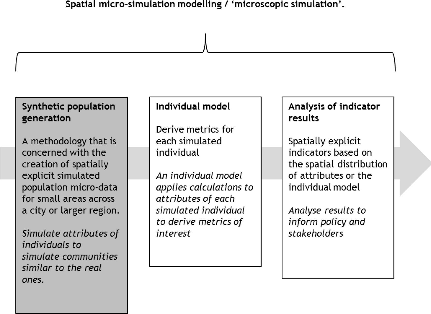
Spatial microsimulation is a well-established method for estimating attributes of individuals when such information is not known or not available. It links data on the distribution of individual characteristics with fine level spatial data to generate synthetic populations. Its history is well documented (Birkin & Clarke, 2011; Clarke, 1996; Tanton, 2014; Tanton & Edwards, 2013). Spatial microsimulation can be dynamic estimating change in each location over time, or static, examining only a single point in time. This paper is concerned with static spatial microsimulation only. A range of spatial microsimulation techniques have been developed for building static models (Tanton, 2014). Spatial microsimulation is also known as synthetic population generation and forms the first part of a larger spatial microsimulation modelling process (Figure 1).

The phases of the spatial microsimulation modelling process. In this paper we are concerned with proposing a hybrid technique for synthetic population generation.
Most spatial microsimulation applications in geography are based on the spatial representation of an attribute of interest found in a single micro-data sample. Examples include the estimation of the geography of smoking or obesity using a health survey (which gives these characteristics for individuals by age, sex, social class, etc.), linked to small-area census of population (which links the individuals with those attributes to small-area geographies). More examples will be given in Sections 2.1 and 3.1. The application area that we are concerned with falls into the broad field of interest of urban sustainability. We will compute a novel measure of the capability of individuals to make journeys by walking and cycling which is an ‘indicator’ of a population’s resilience to transport disruption.
The indicator, which we define fully in Section 2.2, falls into a particular group of policy analysis models which require a synthetic population of individuals as an input and have the following characteristics: (i) results should be available for small zones (e.g. UK Census Output Areas (OAs)1), (ii) the majority of attributes are found in an available micro-data survey, though some attributes are missing and these are available from other sources. The resulting simulated individuals will therefore have many attributes. We refer to this particular group of policy analysis models later in the paper as ‘models of interest’.
Although there are examples of studies which describe techniques that can generate synthetic populations where data about individuals come from multiple sources (e.g. sample free synthetic reconstruction and imputation discussed Section 3), this type of technique is rarer in quantitative geography. In order to address these particular features, we propose a hybrid spatial microsimulation approach. The hybrid approach combines a first stage, in which the majority of the required attributes are simulated (those available from a micro-data-survey), with a second stage in which the missing attributes are added by Monte-Carlo sampling using data from other sources. The first contribution of the paper is therefore methodological, in terms of setting out the details of the hybrid approach, which we believe has wider applications. The second contribution is in terms of the novelty of the application, and in particular the indicator of the resilience of urban areas to fuel unavailability. Additionally, the staged approach means that the intermediate steps in the spatial microsimulation modelling process generate data that are useful in their own right. We have to generate individual and OA level estimates of bicycle availability and the need to escort children to school as part of commuting. To the authors’ knowledge these data have not been synthesised previously at this spatial resolution.
Before explaining the hybrid technique used here, we first introduce the application area and case study data in Section 2, explaining what we are trying to simulate and illustrate how it fits into the class of models of interest. In Section 3 we then discuss existing techniques and offer a rationale for our proposed technique. Section 4 describes the construction of the hybrid technique. Section 5 covers model assessment using established validation methods. Section 6 presents case study results, and Section 7 a summary and areas for further work.
2. Application area, indicator definition and case study data
2.1 Application area
Useful groupings of spatial microsimulation applications include ‘social science focused, spatial microsimulation’ (which include applications within geography as a discipline) and ‘transport microsimulation’ (O’Donoghue, Morrissey, & Lennon, 2014). Applications in the former group include investigations of health inequality (Campbell, 2011; Edwards & Clarke, 2012; Smith, Clarke, & Harland, 2007), estimations of small area income deprivation (Anderson, 2012; Miranti, Cassells, Vidyattama, & McNamara, 2015) and investigation of the local effects of major changes in employment (Ballas & Clarke, 2001). Spatial microsimulation is particularly suited to assessing variation in the populations of particular areas and assessing the extent to which they are likely to be affected by policies. This makes it an effective spatial policy modelling tool, and there remains much potential to take greater advantage of this method to simulate the impact of policy change (Ballas, Dorling, Rossiter, Thomas, & Clarke, 2005; O’Donoghue et al., 2014).
Transport microsimulation is widely used to generate a population of individuals for use in activity based models. Such models take behavioural data to forecast travel patterns and demand over a city or region (Barthelemy & Toint, 2015; Barton, Thompson, Burgess, & Grant, 2015; Beckman, Baggerly, & McKay, 1996; Guo & Bhat, 2007; Huynh, Perez, Berryman, & Barthelemy, 2015; Ma, Heppenstall, Harland, & Mitchell, 2014; Müller, Axhausen, Axhausen, & Axhausen, 2010). As a typical example, the ILUTE model integrates the simulation of the land-use and transport environment and their development over time (Salvini & Miller, 2005), given input data (census data, activity survey data, travel survey data and land-use data).
The sustainable transport literature suggests a continuing need to develop more and better indicators of the benefits of walking and cycling in order to encourage transport and planning policies which fully exploit the use of walking and cycling to contribute to more sustainable cities (Handy, van Wee, & Kroesen, 2014; Larsen, Patterson, & El-Geneidy, 2013). There exists considerable evidence of the benefits of increasing the level of walking and cycling especially in urban areas. These include the promotion of more sustainable modes of transport (Pooley et al., 2011; Jones, 2012), the reduction of car dependence (Buehler & Pucher, 2011), reducing CO2 emissions (Pooley et al., 2012), improvements in health (de Hartog, Boogaard, Nijland, & Hoek, 2010; Ogilvie et al., 2007; Woodcock et al., 2009), increasing the liveability of cities (Burden, 1999; Pikora, Giles-Corti, Bull, Jamrozik, & Donovan, 2003) and reducing congestion (Cervero, Sarmiento, Jacoby, Gomez, & Neiman, 2009; Heinen, van Wee, & Maat, 2010).
Current models which include some consideration of capability to walk or cycle are predominantly based on observations of existing cyclists (Philips, 2014). A model of a population’s capability to make journeys would, on the other hand, allow a greater consideration of those who do not currently make walking or cycling journeys. This could contribute to a more in depth understanding of walking and cycling (Pooley et al., 2011) and would help to ascertain which policy interventions may have a positive impact.
2.2 The indicator being estimated
We wish to estimate the following indicator: The proportion of working individuals aged 16–74 in an Output Area who have the physical capability to commute to their current place of work by walking or cycling given bike availability, their need to escort children to school and assuming no motorised tranport is present on the network.
This is a ‘base-case’ indicator of the population’s resilience to disruptions of the transport system (Philips, Watling, & Timms, 2013) without any policy intervention which henceforth we refer to as ‘the indicator’. In principle the indicator might be directly estimated from survey data; however, we believe such an approach to be unsuitable for several reasons. Firstly the data is highly personal and sensitive and it is not placed in the public domain for reasons of confidentiality (Hermes & Poulsen, 2012). Secondly, fine-grained, small area reporting is especially important for a walking and cycling indicator, as journey distances are generally short (Iacono, Krizek, & El-Geneidy, 2010). This is a finer spatial resolution than direct use of survey data can conventionally provide. For example, large surveys such as the Health Survey for England (HSE) typically have respondents from all regions, but not for all smaller zones within each region (Craig, Mindell, & Hirani, 2009). In these cases the sample size for sub-district level analyses would typically be so small to be subject to large margins of error. For example, when the Active People Survey data was analysed to produce estimates using the UK census geography – Middle Layer Super Output Areas (MSOA) , the researchers themselves expressed concern over the high margins of error in some areas (IPSOS MORI, 2007).
Instead, we propose to estimate the indicator using spatial microsimulation. We believe this, rather than a more aggregate level model, is especially justified in our application for several reasons. Firstly, excessive aggregation in policy analysis can be problematic, with a ‘one size fits all’ approach to policy leading to dilution of investment, untargeted interventions and poor outcomes (Ballas et al., 2013; Openshaw, 1995). Individual level modelling allows small unit reporting, which, also goes some way to alleviating the modifiable area unit problem (Openshaw, 1984), and by making analysts mindful of the heterogeneity of areas helps to avoid the ecological fallacy. Secondly there is individual variation across multiple attributes, which interact to influence the indicator and aggregate data based on; for example the mean attribute value would fail to adequately consider this variation. Locating concentrations of individuals at the extremes of the distribution of capability is likely to be of particular interest to policy makers. Taking the national mean of individual attributes would be an inadequate measure, as it would not help identify those key people at the extremes of the distribution of capability. For this reason, even disaggregation by age and gender (for example, taking the average fitness level for population segments such as men over 50) may be too coarse.
2.3 Case study data
This case study falls into our class of models of interest. Firstly, the synthetic population has to represent many attributes. Table 1 defines the wide range of data sources required to produce the indicator. Not all the required attributes are available in a single micro-data sample, most are available in the HSE anonymised micro-data, the other attributes are found in other data sets. Secondly, the case study includes all the phases of spatial microsimulation modelling (Figure 1). In the first phase (synthetic population generation) attributes are simulated directly from the data. Phase 2 takes the synthesised attributes produced in phase 1, from which further attributes can be derived such as VO2max2 (ml/litre of blood/kg body mass) and pedalling power. Local environmental variables representing features such as topography and wind are then also introduced. The individual model then estimates an individual’s capability to make walking and cycling journeys. The second modelling phase (Shown in Figure 1) is discussed in Section 3 below and in detail in Philips, (2014) and Philips, Watling, Timms, (2015). The case study also illustrates the third phase shown in Figure 1 by demonstrating the ability to visualise and analyse the spatial distribution of specific attributes as well as the spatial distribution of the indicator.
Attributes and data sources used in Phase 1 (synthetic population generation) of the spatial-microsimulation modelling process.
| Variable | Data source | Possible values | Constraint | Stage * |
|---|---|---|---|---|
| Physical activity (days in last 4 weeks with 30+mins vigorous activity) | HSE | 0–28 | N | 1 |
| Body Mass Index (kg/m2) | HSE | 15–48 | N | 1 |
| Age group | Census: Table CS028 Sex and Age (16–74) by Economic Activity & HSE | 16–24, 25–34, 35–54, 55–64, 65–74. | Y | 1 |
| Gender | Census table CS028 & HSE | M/F | Y | 1 |
| Weight (kg) | HSE | 32–130kg | N | 1 |
| Bicycle availability | NTS /(Anable, 2010) | Probability given age, gender and NSSEC | N | 2 |
| The need to escort children on commute | NTS / Children & Early Years Survey, 2010 | Probability given age and gender | N | 2 |
| Current commute distance | Census table CAS120 | Bins, 0, 0–2, 2–5, 5–10, 10–20, 20–40, 40–60, < 60, not fixed. | Y | 2 |
| Economic activity | Census table CS028 & HSE | Working, unemployed, student, economically inactive. | Y | 1 |
| LLTI | Census table CS021 and HSE | Y/N | Y | 1 |
| Highest educational qualification | Census table KS013 and HSE | 6 categories | Y | 1 |
| NSSEC by sex | Census tables KS014 b and c. & HSE | 10 NSSEC categories by gender | Y | 1 |
-
Source: Health Survey for England, 2008 (HSE), National Travel Survey (NTS), UK Census, 2001, Limiting Long Term Illness (LLTI), National Statistics Socio-Economic Classification (NSSEC).
-
Notes: * The column ‘Stage’ refers to the simulated annealing Stage 1 or Monte-Carlo sampling Stage 2 of the synthetic population generation phase described in Section 4.
3. Existing techniques and rationale for hybrid spatial microsimulation technique
3.1 Existing techniques for generating synthetic populations
The most common techniques of spatial microsimulation may be grouped as several broad categories. The first category comprises synthetic reconstruction which generates populations based on joint conditional probabilities of attributes (e.g. Clarke, 1996). Synthetic reconstruction requires as a minimum the probability of each attribute category occurring. Probabilities can be derived from a sample of individual records or using a sample free approach. To be of practical use there should be conditional probability distributions for the occurrence of each attribute combination. Secondly one or more constraint tables are needed. A constraint table is a table of data from the census. It contains counts of the number of people with a particular attribute resident in a particular area; for example a table listing age group by gender. This allows synthetic reconstruction by estimating gender given the age of an individual and the conditional probability distribution.
The most common way of implementing synthetic reconstruction is using iterative proportional fitting and Monte-Carlo sampling (Beckman et al., 1996). Alternative implementations in this category include models simulating at two micro-levels (e.g. household and individual, see Arentze et al., 2007; Guo & Bhat, 2007; Ye et al., 2009) and secondly models which take a sample free approach (Barthelemy & Toint, 2013; Gargiulo, Ternes, Huet, & Deffuant, 2010). Lenormand and Deffuant, (2013) compared the models of Ye et al., (2009) and Gargiulo et al., (2010). They found the sample free approach performed better, it was also less data demanding though it did require more pre-processing than sample based synthetic reconstruction. Barthelemy & Toint, (2013) found the sample free approach performed better than the sample-based method of Guo and Bhat, (2007).
A second major category of techniques is, combinatorial optimisation. Such methods select all the attributes of an individual from anonymised individual survey records (such as the HSE micro-data described in Section 2.3) and ‘clones’ combinations of these individuals to match the aggregate counts of attributes for each zone given in the census. The main algorithms for combinatorial optimisation are deterministic reweighting (Ballas, Dorling, et al., 2005) and simulated annealing (Harland, Heppenstall, Smith, & Birkin, 2012; Rahman, Harding, Tanton, & Liu, 2010).
The data requirements for combinatorial optimisation are firstly a micro-data survey (also called a sample population): a table containing data about individuals taken from a survey such as the HSE. Combinatorial optimisation also requires constraint tables. Constraint attributes (called constraints) are those which are common to both the census constraint table and the sample population. For example both the uK census and the HSE contain data on age and gender.
The class of spatial microsimulation application we are interested in also requires unconstrained attributes (we are interested in models requiring a large number of attributes). For example, there are no tables in the UK census which describe the amount of vigorous exercise people do. This data is only found in the HSE micro-data survey. However, age and gender are correlates of frequency of vigorous exercise (McArdle, 2010) so they are suitable to be used as constraints.
Williamson, (2012) compared simulated annealing and synthetic reconstruction using 1991 census data. The overall assessment by Williamson, (2012) was that simulated annealing was the best performing method. Harland, et al., (2012) compared simulated annealing, deterministic reweighting and synthetic reconstruction techniques when given the same input data and constraints using uK data and found simulated annealing performed best at the finest spatial resolution. These comparisons however are anterior to the most recent developments in sample free synthetic reconstruction so it is possible that the best performing method may change over time.
There are other practical benefits to using combinatorial optimisation techniques. Firstly, the synthetic population only needs to be constructed once, whereas synthetic reconstruction populations need to have multiple iterations (i.e. generate multiple populations) because of the greater variation. This gives combinatorial optimisation methods both a computing time and a data storage benefit (Williamson, 2012). Additionally combinatorial optimisation more easily allows the inclusion of unconstrained attributes (Hermes & Poulsen, 2012). Populations generated using a sample population have a further advantage when used for policy analysis. A sample population such as the HSE records a great many attributes for each individual, in some circumstances3 the spatial distribution of these extra attributes can be analysed to widen the range of policy questions that can be addressed without having to rebuild the synthetic population. There is a further issue raised by synthetic reconstruction and deterministic reweighting methods namely, the order in which constraints are added has an effect on the outcome thus introducing further complications (Clarke, 1996; Huang & Williamson, 2001).
Even if we were to assume that simulated annealing is the currently best performing technique, there are reasons to use other techniques in some circumstances. Deterministic reweighting is computationally less intensive than the other techniques (Hermes & Poulsen, 2012). Synthetic reconstruction is useful in the absence of a sample population (Huynh, Barthelemy, & Perez, 2016). Combinatorial optimisation methods require that the constraint tables be available at the same scale; that is all constraints have to be available at OA resolution if the model is to be built at that scale (Barthelemy & Toint, 2013; Ballas et al., 2005a). Extra processing of constraint tables is required to overcome the deliberate errors introduced to preserve anonymity at fine resolutions (Stillwell & Duke-Williams, 2003).
A third and final category is that of imputation methods (Lymer, Brown, & Yap, 2009; Schofield et al., 2015). Such methods, while less common, are particularly relevant to the current study, as there exist examples in which imputation is used to generate a synthetic population when not all the data is in a single micro-dataset. In the case of two micro-data sets, the general approach would be to separately generate two synthetic populations for each small area (based on the two sets of micro-data), and then ‘impute’ attributes from one population onto the other. Schofield et al., (2015), for example, generate two synthetic populations for the same year: (i) Health&WealthM0D2030, generated using GREGWT, to reweight to the 2010 population; and (ii) APPSIM, a dynamic spatial microsimulation based on reweighting using a synthetic population for 2010. They then impute values using synthetic matching from APPSIM (the ‘donor’ synthetic population) into Health&WealthM0D2030 (the ‘recipient’ synthetic population), with the resulting synthetic population being then used for policy analysis. Lymer, Brown, & Yap, (2009) use regression-based imputation to address a slightly different problem. They have a micro-data sample containing all the attributes of interest, but the population sub-group they wish to analyse is underrepresented in the data.
3.2 The proposed hybrid spatial microsimulation technique
Our proposed hybrid technique for the synthetic population generation phase has two stages. Stage 1 uses simulated annealing based combinatorial optimisation to simulate the majority of the required attributes. Stage 2 uses Monte-Carlo sampling to add individual attributes which were not available in the sample population. The main steps in the algorithm are shown in Figure 2:

The main steps in the algorithm.
Our rationale for this hybrid technique is as follows: the hybrid technique allows the full range of desired attributes to be modelled rather than having a model restricted by limited data sources which would be the case if we only used combinatorial optimisation. We use simulated annealing as it has been proposed as the best performing technique when applied to small areas, though we acknowledge that continuing developments mean that this may not remain so indefinitely.
Simulated annealing however requires that all attributes to be simulated are found in the same micro-data sample. In our application, it is not possible to find all the attributes in the same micro-data sample. Additionally, commute distance cannot be assigned to an individual until that individual has been allocated a location. Commute distance is strongly associated with location as well as individual socio-demographic attributes. Commute distance is collected in some micro-data surveys, but, it would not be appropriate to allocate this value out of its original spatial context as individual survey data has geographical detail removed, meaning that we would not be able to ensure that we connect a simulated individual to an appropriate commute distance based on the area to which they are assigned.
Synthetic reconstruction can be applied where a micro-data sample is not available. However using it alone would forgo the reported performance advantages of simulated annealing at the smallest geographies as well as neglecting the practical benefits of not having to consider the order of constraints or the potential for adding additional attributes to individuals. The imputation approach appears to be a practical solution where existing appropriate synthetic populations are available, but this may not always be the case. In some cases a population may already exist containing most attributes required, and the hybrid technique may take what is in effect a partially constructed population and add to it. Another option is that there may be a number of micro-data sources. In some cases it might be quicker to use a hybrid technique rather than generate a synthetic population for each micro-data source then undergo multiple iterations of imputation. In these cases sample- free synthetic reconstruction may be better suited for some applications, but there remain some applications where the user wishes to use combinatorial optimisation. Introducing Monte-Carlo sampling in the second stage of our technique creates a source of stochastic variation. This is not a problem if a suitable number of iterations are made; the standard error of the mean should not be excessive.
The technique we propose is a distinct means by which our ‘models of interest’ could be produced combining these candidate best performing techniques, this is explained more fully in Section 4. We must stress that the purpose of this paper is not to compare the performance of our technique to imputation or sample free synthetic reconstruction techniques (though that is an area for further research) but to describe the technique and demonstrate its implementation to a ‘model of interest’. Table 2 summarises the ways in which our proposed hybrid technique is distinct from other techniques discussed above.
Summary of how proposed technique is distinct from other techniques.
| Technique | Comment on suitability for use on model of interest | How our proposed hybrid technique differs |
|---|---|---|
| Single-stage simulated annealing Deterministic reweighting Sample-based synthetic reconstruction | Not suitable because not all data in the model of interest is in one micro-data sample | Can deal with individual attribute data from multiple sources |
| Sample-free synthetic reconstruction | This may be suitable as it can handle data from multiple data sources and current developments mean it may be effective at simulating populations at the finest resolution | Specifically seeks to incorporate simulated annealing (rationale in text of Section 3.2) |
| Imputation using multiple existing synthetic populations | This may be suitable if it is accurate at simulating populations at the finest zones, and may be useful where there are existing synthetic populations | May be useful where suitable populations are not available |
| Imputation to better simulate under-represented individuals in a single micro-data sample | Not suitable on its own because not all data in model of interest is in one micro-data sample | Hybrid technique can deal with individual attribute data from multiple sources. We model stochastic variation in pedal power through cloning. Lymer, et al., 2009 also use a cloning approach which may inform future developments of our technique |
our proposed technique is one of a set of approaches that produce synthetic populations where not all data are available in a single micro-data sample. our technique is distinct from the imputation work of Schofield et al., (2015) and Lymer et al., (2009) described above. We use Monte-Carlo sampling to represent heterogeneity in the micro-data sample whereas Lymer et al., (2009) use regression based imputation. We use Monte-Carlo sampling in Stage 2 of our synthetic population generation to synthetically construct missing variables using conditional probabilities e. g. the probability of an individual having a bike given age, gender and social class. In our technique however we do not use complete conditional probabilities using all attributes generated in Stage 1 (see Section 4.3 for details). We note the proposed technique is also distinct from methods that seek to generate synthetic populations constrained on both individual and household level attributes simultaneously.
4. Development of the technique
4.1 Pre-processing of the micro-data sample and constraint tables
The data used for our study are shown in Table 1.
A sample population of micro-data is based on the 2008 HSE. It contains the attributes BMI (Body Mass Index), level of vigorous exercise, weight, age and gender. The latter two are needed to calculate the indicator, as well as being constraint attributes. Cyclist pedalling power was estimated for each individual in the sample population, using the method described in Philips, Watling, and Timms (2015). Cycling pedalling power is assumed to be a function of maximum exertion, as measured by VO2max, which was derived by a regression model using empirical data based on: age, gender, BMI and level of vigorous exercise (Wier, Jackson, Ayers, & Arenare, 2006), as well as the maximum level of exertion which can be sustained for the duration of a commute. In the pre-processing of the sample population, each individual in the micro-data sample was cloned 10 times, and VO2 max estimated for each clone from a distribution based on the Standard Error of the Estimate in Wier et al’s model. The output at this point is a sample population based on the HSE which accounts for the conditional nature of Vo2max and pedalling power.
The choice of constraints for Stage 1 was made firstly by examining correlations with unconstrained attributes of interest (BMI and physical activity), as is standard practice (Cassells, Miranti, & Harding, 2012). Age and gender are associated with BMI and physical activity (McArdle, 2010). Obesity is found to be related to Limiting Long term Illness (LLTI) and National Statistics SocioEconomic Classification (NSSEC) (NOO, 2010). NSSEC and education are also associated with physical activity (IPSOS MORI, 2007). The constraints used in full are: Age, Gender, Economic Activity, LLTI, Education, NSSEC. The OA tables used as constraints required extra processing to overcome the deliberate errors that had been introduced into the source data in order to preserve anonymity at fine resolutions (Stillwell & Duke-Williams, 2003). The population totals in each OA were not consistent across all constraint tables, and so a balancing and integerisation procedure was developed, as shown in the first block of pseudo code below (Algorithm 1), whereas the second block accounts for rounding losses:
Pseudocode.
|
1: Select reference population table 2: Calculate cell value based on frequencies: 3: Raw cell value / raw row total) * reference population total 4: Intergerise the decimal value from the previous step: Round the value up or down 6: If rounded value ≠ reference population total then 7: If reference population total < integerised row total then 8: subtract 1 from a random cell in the row 9: If reference population total > integerised row total then 10: add 1 to a random cell in the row. 11: Repeat until rounded value = reference population total |
Census tables and HSE data were pre-processed using SPSS scripts, Excel and VBA (Visual Basic for Applications) into a format that could be used by the Flexible Modelling Framework (FMF) simulated annealing software built by Harland (2013). The output at this point is a set of constraint tables which all have consistent population totals, and with categories which are consistent with categories in the HSE sample population.
4.2 The hybrid technique Stage 1 (simulated annealing based combinatorial optimisation)
Stage 1 uses simulated annealing based combinatorial optimisation. The inputs are the sample population based on the HSE and the constraint tables based on the census which were described in Section 4.1. For a detailed description of the simulated annealing algorithm and the Java program FMF see Harland, (2013). The output at this point is simulated values of all attributes listed as ‘Stage 1’ in Table 1. The FMF represents this by producing the FMFRESULT table. Each row represents an individual, the first field contains a reference to an OA and the second field contains the identifying reference to the row in the sample population that specifies all the attributes for the cloned individual.
4.3 The hybrid technique Stage 2 (Monte-Carlo sampling)
Stage 2 is outlined in Figure 3. Stage 2 uses Monte-Carlo sampling to add two individual attributes which were not available in the sample population; bicycle availability and the need to escort children on the way to work. It also adds commute distance which is a geographically dependent attribute; it is only allocated once it is known where an individual lives.

Stage 2 of the hybrid microsimulation technique using Monte-Carlo sampling.
The output from Stage 1, the FMFRESULT table was read into a MySQL database along with the SAMPLEPOPULATION and GEOGRAPHIC_FACTORS tables. The COMMUTE_CDF table containing the cumulative distribution function (cdf) was read in having been generated as follows from the 2001 census table CAS120:
Read in CAS120 commute distance by gender by age group fields: zone, 0–2 km,… > 60km]
Convert to cumulative distribution table for each gender by age group [e.g. male aged 16–24, male aged 25–34 … female 70–74 ].
A subset of the population, namely those who were in employment and aged 16–74, formed the table EMPLOYEES, whereas the table COMMUTE_CDF_EMPLOYED contained the corresponding cumulative probability distribution table of commute distances for this population subset (the distances discretised into ‘bins’). The table MAXDISTOPTIONS contained one row per individual from the table EMPLOYEES, specifying the maximum distance that an individual could travel (i) with a bicycle and without needing to make an escort trip, (ii) with a bicycle and having to make an escort trip, (iii) by walking without needing to make an escort trip and (iv) by walking and having to make an escort trip.
The function used to estimate the maximum travel distance for each individual was based on Wilson, (2004), and is described in detail in Philips, (2014). For each Monte-Carlo sampling iteration (up to a total of Ntotal iterations), the tables COMMUTE_DISTANCE_DRAW_N and MAXIMUM_DISTANCE_DRAW_N were calculated, as shown in the first and second blocks respectively of the pseudocode below (Algorithm 2):
Pseudocode.
|
1: For Ntotal iterations 2: CREATE TABLE COMMUTE_DISTANCE_DRAW_N 3: For each gender by age group 4: For all individuals in EMPLOYEE table who are in this gender by age group 5: Set commute distance bin by drawing a random number between 0 and 1 and comparing it to the cumulative proportion in the cumulative distribution table 6: Set the commute distance = 7: minimum distance in bin + (random number [0–1] * maximum distance in bin). 8: For Ntotal iterations calculate the maximum distance the population can travel 9: CREATE TABLE MAXIMUM_DISTANCE_DRAW_N for iteration N 10: SELECT data from SAMPLEPOPULATION & EMPLOYEE (this table contains probability of bike availability given Stage 1 attributes and probability of escort trip given Stage 1 attributes) 11: WHERE the probability of having a bike > [random number between 0 and 1] set individual has bike = 1 12: WHERE the probability of having to escort children to school > [random number between 0 and 1] set individual has to escort children = 1 13: UPDATE MAXIMUM_DISTANCE_DRAW_N [Calculate maximum distance each individual is capable of travelling] |
Once the maximum distance and commute distance for an iteration was calculated, each individual’s capability to travel was calculated as shown in the first pseudocode block below (Algorithm 3). In the second block the capability of all individuals in each OA was then summarised for iteration N:
Pseudocode.
|
1: For Ntotal iterations 2: CREATE TABLE INDIVIDUAL_RESULT_DRAW_N 3: JOIN commute distance draw N and maximum distance draw N 4: For each individual 5: Capability to commute = 1 where maximum distance – commute distance >= 0 6: Capability to commute = 0 otherwise. 7: CREATE TABLE INDICATOR_result_draw_N (fields: Output Area ID, sum of people with capability to commute, % of employed population with capability to commute). |
We have generated multiple populations and they are stored as follows: The attributes generated by the FMF software in Stage 1 are common to all populations. They are stored in the EMPLOYEE table. The attributes generated in Stage 2 which differ from one population to the next are stored in the INDIVIDUAL_RESULT_DRAW tables. Each population has a number between 1 and Ntotal. The number of individuals in each OA in population N with the capability to commute is recorded in INDICATOR_RESULT_DRAW table N. When all iterations are complete, the results of all iterations are summarised by calculating the mean estimate of the percentage of the population in each OA with the capability to commute by walking or cycling (all individual results were also retained in the database). The database allows easy storage of the resulting tables; it was possible to simulate the attributes of all 21 million working individuals in all of the ~165000 OAs in England. The database was used to calculate the results of the individual model and output the results aggregated to OA zones as CSV files, a format easy to use in GIS (Geographical Information Systems) and statistics packages to map and graph the results. The multiple output populations reflect the conditional nature of the data and are shown in Table 3.
Synthetic population outputs.
| Output | Table | Attributes |
|---|---|---|
| Ntotal synthetic populations of individuals | INDIVIDUAL _RESULT_DRAW_N | Physical activity, BMI, age, gender, weight, bicycle availability, need to escort children on commute, pedalling power, maximum travel distance, commute distance, capability to commute by walking or cycling. |
| Ntotal summaries of the % of the working population in an Output Area capable of commuting by walking or cycling | INDICATOR_RESULT_DRAW_N | Zone code, % of population capable of commuting by walking or cycling |
| Summary of capability of all populations at Output Area resolution | INDICATOR_RESULT_DRAW_SUMMARY | Zone code, % of population capable of commuting by walking or cycling for each iteration, mean capability for all populations, standard deviation of capability for all populations |
5. Model assessment: assessing the performance of the hybrid technique
To assess the error in generating a synthetic population, we carried out internal and external validation tests (Edwards & Tanton, 2012), and also estimated the extent to which each stage of the spatial microsimulation contributed to uncertainty in the estimate of the indicator. To prepare the synthetic population for validation, we aggregated it to the same resolution as the constraint tables, which in this case was OAs.
Firstly we performed internal validation tests of attributes that were common to both the constraint tables and the sample population. The internal validation process indicates the extent to which the synthetic population’s attributes match the aggregate counts of the real population’s constrained attributes. The results are summarised in Table 4. These showed the poorest fitting constraint to be NSSEC by gender, a 20-class, cross-tabulated constraint (percent cell error value of 9.2). We reconstructed this constraint as a uni-variate constraint with only 3 NSSEC categories, and this greatly reduced the percent cell error. The percent cell error of the simulated annealing stage constrained attributes was an average of 0.065% per attribute using the 3 category NSSEC constraint. This compares favourably to that achieved by Harland et al., (2012), who achieved zero error for constrained attributes at OA resolution, whereas the synthetic reconstruction and deterministic reweighting average error per constraint was 0.96% and 14.15% respectively (source Harland et al., 2012 in their Table 3). In Stage 2 the commute distance attribute is available in the census, so can be internally validated. The mean percent cell error was 0.76% per attribute, performing well when compared to Harland et al., (2012). We calculated the indicator using both constructions of the NSSEC constraint. This is an approach to estimating error arising from the specification of spatial microsimulation models (O’Donoghue et al., 2014; Smith et al., 2009). The difference in indicator value was used as an estimate of the level of uncertainty arising from the configuration and specification of constraints. In 95% of OAs the uncertainty in the indicator arising from stage 1 was >= 4.8%.
Summary of internal validation tests.
| Variable name | Percent cell error |
|---|---|
| Sex by age by economic activity | 0.065 |
| Education | 0.065 |
| LLTI | 0.065 |
| NSSEC with 3 categories | 0.065 |
| Commute distance by age by sex | 0.76 |
External validation of unconstrained attributes in spatial microsimulation models is typically very difficult, since the reason for using spatial microsimulation in the first place is a lack of data covering all the attributes of interest at the spatial resolution and extent required, leaving little or no data available to validate against (Edwards & Tanton, 2012). We carried out tests on three unconstrained variables; obesity (an element of BMI), bike availability, and those not engaging in any sport or vigorous exercise (an element of physical activity). The results are shown in Table 5.
Results of external validation tests.
| Unconstrained attribute | Results compared |
|---|---|
| BMI (Obesity used as a proxy) | % of adult population classified as obese |
| Public Health England (PHE) national estimate (HSE data, 2006 — 2008) | 24.2 |
| Synthetic population using hybrid technique | 23.9 |
| Bike availability | % of adult population with use of a bike |
| NTS, 2010 national estimate of bike availability amongst adults. | 37.2 |
| Synthetic population using hybrid technique | 38.3 |
| Physical activity | % of adult population with no participation in sport |
| Active People Survey (APS), people not doing 1x30 minutes sport per week | 57.0 |
| Synthetic population using hybrid technique | 58.7 |
These figures show that the unconstrained variables have small errors in their estimation at a national level. However further validation at a finer resolution would be beneficial.
To test the stochastic uncertainty introduced by Stage 2 (the Monte-Carlo sampling) for each OA we calculated the standard error of the mean indicator value. A small standard error (SEj indicates a low level of stochastic variation in zone j and therefore greater certainty about the indicator value. SEj is calculated by dividing the standard deviation between iterations, σj of the indicator value for each zone by the square root of the number of iterations Ntotal:
In 95% of OAs SEj was less than 1.8%. This gives an estimate of the error in the indicator arising from both stages of the spatial microsimulation in the hybrid synthetic population generation of ±7.6%. The estimate of uncertainty for every OA was mapped and is shown in Figure 4. A small number of OAs (117 of 2439) had an error of over 7.6%.

An estimate of the percentage indicator error resulting from the hybrid spatial micro simulation technique, showing Leeds and surrounds.
6. Results
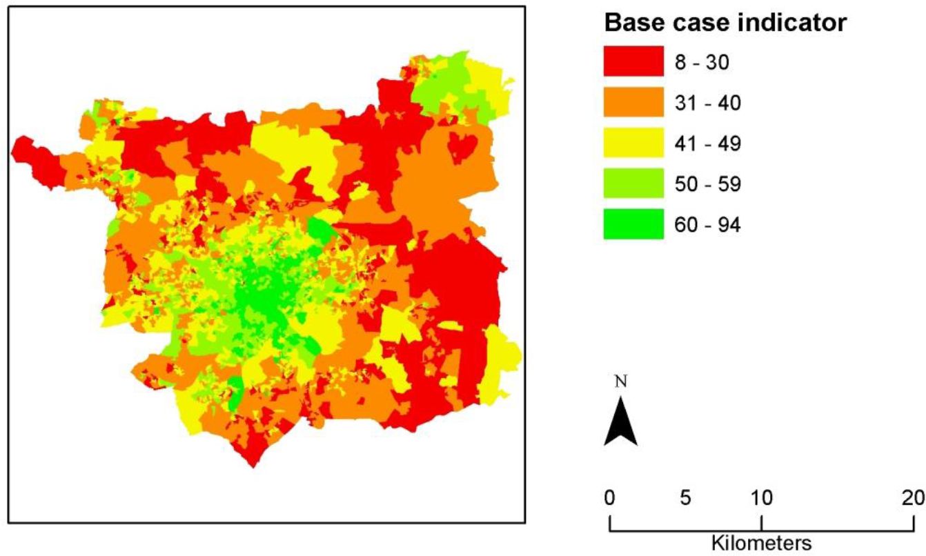
The results of applying our method, in terms of the calculated indicator, are shown in Figure 5. The indicator is highest closer to the centre of the city, which may be expected as it is the largest employment centre (so there will be many short commute distances). There are also some OAs with very high indicator values around the satellite towns of Otley (in the north-west) and Wetherby (in the north-east) This may be due to short commute distances to these sub-centres. However other individual demographic factors may also play a part.

The indicator for Leeds Output Areas. The percentage of working individuals aged 16–74 in an Output Area capable of commuting to their current place of work by walking or cycling.
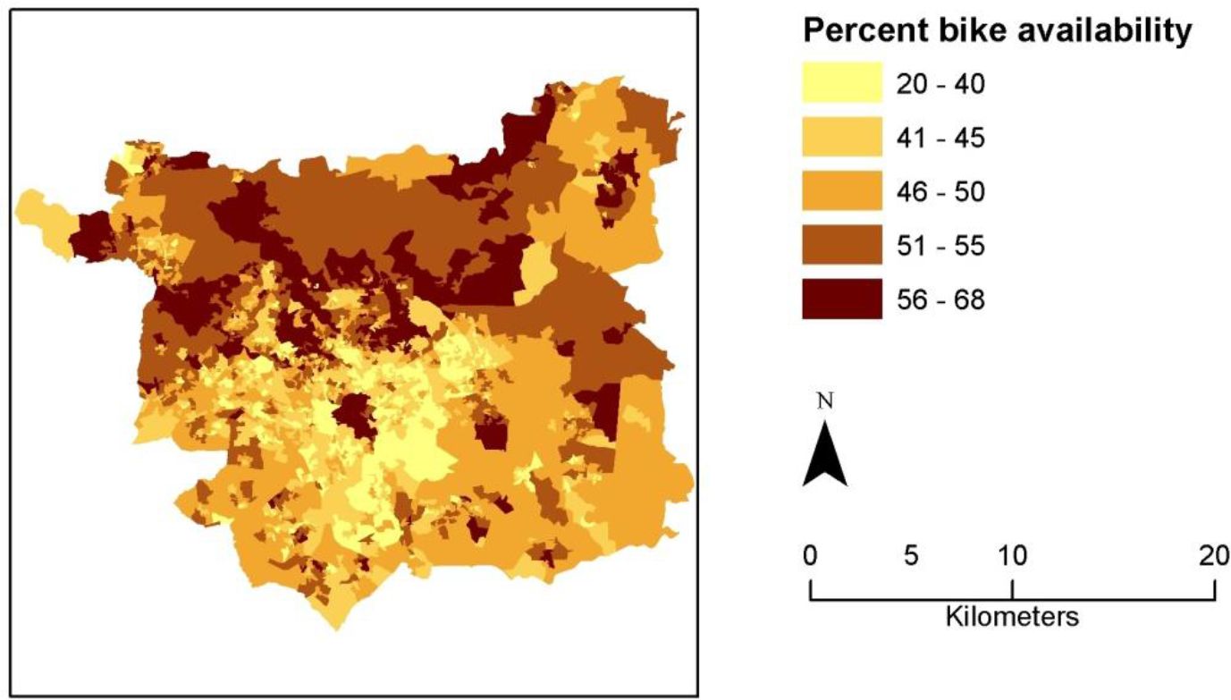
Because we have used a microsimulation approach, we can finally map the distribution of individual simulated attributes. To illustrate this, bike availability is generally higher towards the northern edge of the city and yet the highest levels of bike availability are associated with the lowest indicator values. This may be partially explained by the fact that the north of the district is bounded by the steep valley side of the River Wharfe (and so cycling may require relatively high levels of physical exertion), and that the north of the district has high levels of workers with long commutes. In addition to contributing to estimation of the indicator, estimation of the percentage of bicycle availability at OA resolution (Figure 6) is a potentially useful variable for planning cycle interventions.

Percentage of working population in Leeds OAs with access to a bike.
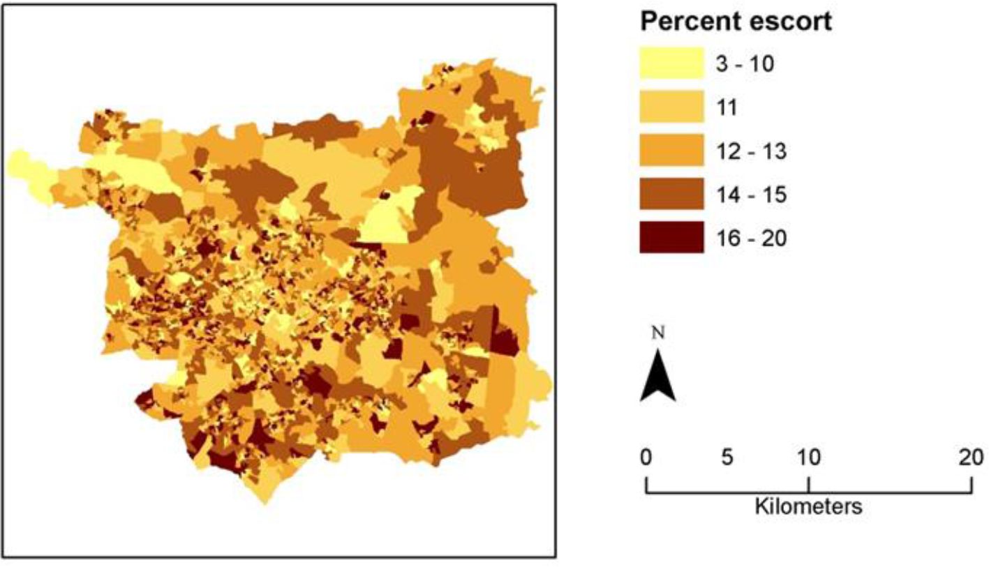
A second new variable created in this application is the proportion of working individuals who have to escort children as part of their commute at OA resolution (Figure 7). The pattern of this variable varies between different neighbourhoods in the city. For example, the city centre and the north-west inner suburbs have high proportions of students and young professionals so may explain the many OAs with low levels of escort trips. As well as contributing to indicator estimation, understanding constraints on travel imposed on those with caring responsibilities could contribute to understanding the social constraints often based on gender and social group that influence the ability to use transport to access activities (Lucas & Jones, 2012).

Percentage of working population in Leeds OAs needing to escort children during the commute to work.
Because we have used a microsimulation approach, we can examine how the individual variables contribute to the indicator in different locations. Providing quantitative data which illustrates variation in processes influencing the indicator could, when used in the context of local geographical knowledge, be useful to planning practitioners. The correlations between individual attributes at city level and the indicator value are shown in Table 6. Within Leeds, gender, age and bicycle availability have the greatest association with the indicator. These correlations would vary if examined at a sub-city resolution.
Correlations of individual attributes with the indicator.
| Attribute | Correlation with indicator value |
|---|---|
| Age | −0.33 |
| % female | −0.58 |
| BMI | −0.156 |
| % obese | −0.132 |
| Pedal power | 0.247 |
| % bike | −0.305 |
| % escort | −0.082 |
| Slope | −0.122 |
| Commute distance | −0.267 |
| Maximum travel distance | 0.077 |
Finally, we examined the spatial pattern of individual attributes in order to explain the spatial pattern of error in the hybrid model. The spatial distribution of uncertainty informs policy makers where indicator results should be treated with greater caution, and may also be used as a basis to target future resources for refining the model (i.e. to reduce error). From the analysis leading to Figure 4, it was seen that many of the OAs with error over 7.6% are in the suburban areas, between 5km and 8km from the city centre. Many individuals in these OAs have a mean maximum travel distance in the range 5–8km and a commute distance in the same range. In OAs where commute distance and maximum travel distance are similar, small errors in the estimation of individual attributes (from which the maximum travel distance is derived) have a larger effect on the error. one attribute from which maximum travel distance is derived is bicycle availability. Comparing Figures 4 and 6 shows, bike availability is high in many of the oAs with high error. Small errors in estimating bicycle availability (as simulated in each iteration of the second stage of the hybrid model) will therefore have a relatively large effect on the estimate of capability of individuals to make journeys in the 5–8km range.
7. Summary and conclusions
In order to summarise the contribution of the work presented, we will refer to the criteria suggested by O’Donoghue et al., (2014) for assessing the quality of spatial microsimulation models: (1) The model links constraint and individual data, either through sampling or simulation. (2) It has the capability to handle units of analysis of interest: either individual, household, or a combination of the two. (3) It should be computationally efficient. (4) It should be transparent. (5) It should minimise validation error.
Our hybrid model makes progress towards (1) by linking spatial data to all the attributes required, for the class of models of interest defined in the introduction. The case study presented handles individuals as units of analysis, thus satisfying criterion (2). The case study describes the distribution of novel policy relevant variables such as bicycle availability and the need to escort children during commuting, in addition to the overall indicator.
Regarding criterion (3), while the reported case-study focused on a particular urban area, the model has in fact been run for the whole 2001 working population of England at, OA resolution (approx. 21 million individuals in approx. 165000 zones) on a Windows laptop with a dual core processor (Intel Core 2 Duo T6500/2.1 GHz) and 4GB RAM. The simulated annealing stage was run using a parallelised Java application (Harland, 2013) taking 4 hours when the simpler 3 way construction of the NSSEC constraint was used and 30 hours with the cross-tabulated NSSEC by gender constraint. The second stage and storage of data used a MySQL database and ran in 48 hours. When simulating only Leeds (the case study reported in the paper), rather than the whole of England, the run time was approximately 30 minutes for Stage 2. Run-times could potentially be reduced through improvements in the coding of the SQL database, though the time required for synthetic population generation is not a major concern as it is typically done only once, and then used as an input to phases 2 and 3 of the microsimulation modelling process shown in Figure 1.
Consolidating all code into a single form so that it is more easily shared and replicable may be a useful piece of further work. Harland’s software is free and open access. We have also explained above the process involved in the two stage generation of the attributes of synthetic individuals, making progress on criterion (4). The internal validation tests reported in Section 5 show that through the choice and construction of constraints, we have sought to minimise the validation error of this application, and so we have also made progress towards criterion (5).
A future development to explore could be to incorporate Lymer et al’s, (2009) approach to modifying the micro-data sample, in order to improve our model in oAs where we observe high standard errors, and to make a comparison of Lymer et al’s approach with that of Smith, Clarke, and Harland (2009). The approach of Schofield et al., (2015) may be useful if we wished to estimate capability to make journeys by walking and cycling in other countries where existing synthetic databases exist, and which (if combined with our approach) could provide the attributes needed to analyse capability to make journeys by walking and cycling. It would be useful to test our model more formally against the best performing sample-free synthetic reconstruction methods and imputation approaches, to gain further understanding of the construction of attribute-rich, synthetic populations in small zones.
A further application/development of our methods could be in accounting for a greater range of household constraints on travel, for which we might generate a synthetic population of individuals linked within households. Surveys such as the HSE contain data which would allow linking of individuals in households. The ability to incorporate innovations in linking household and individual populations (e.g. Arentze et al., 2007; Guo & Bhat, 2007; Ye et al., 2009) may also be worthwhile to consider in any extension of Stage 2 of our hybrid approach to deal with household-level constraints.
In this paper we have explained how to estimate our indicator. It is a ‘base-case’ indicator constructed from existing data rather than a counter-factual scenario. It would also be possible to estimate a counter-factual ‘policy case’ indicator based on ‘what-if scenarios, in which the attributes of individuals affected by the policy would be altered. This would require the indicator value to be recalculated, for each iteration of the synthetic population. As all populations generated for the base case indicator are retained in the database, along with random number seeds, we need not introduce any additional stochastic noise (by using ‘common random numbers’). This would mean that the base case synthetic population would not be stochastically different to the policy case synthetic population (Rathi, 1992; Stout & Goldie, 2008), thus aiding comparison between the base case and policy case indicators.
Footnotes
1.
Output Areas (OAs) are the smallest UK census dissemination zones with median extent of 7ha, containing ~125 households and are designed to group socio-demographically similar households. https://www.ons.gov.uk/methodology/geography/ukgeographies/censusgeography
2.
VO2max (measured in ml per minute per kg of body weight) is a measure of a person’s maximum oxygen uptake. It is used as an indicator of cardio-vascular endurance and can also be used to calculate a person’s energy use and power output during exercise (McArdle, 2010).
3.
It is not always appropriate to do this; for example if the extra attributes are not correlated with the constraint attributes.
References
-
1
Monitoring and Evaluation of the Smarter Choices Smarter Places Programme. Working paper 2010/01. Analysis of walking and cycling activity and its relationship to social-economic status (Working paper)Scottish Government.
-
2
Estimating Small-Area Income Deprivation: An Iterative Proportional Fitting ApproachIn: R Tanton, K Edwards, editors. Spatial Microsimulation: A Reference Guide for Users. Springer Netherlands: Dordrecht. pp. 49–67.
-
3
Creating Synthetic Household Populations: Problems and ApproachTransportation Research Record: Journal of the Transportation Research Board, 2014 pp. 85–91.
-
4
SimBritain: a spatial microsimulation approach to population dynamicsPopulation, Space and Place 11:13–34.
-
5
Spatial Microsimulation for Rural Policy Analysis35–54, A Review of Microsimulation for Policy Analysis, Spatial Microsimulation for Rural Policy Analysis, Springer Berlin Heidelberg, http://link.springer.com/chapter/10.1007/978-3-642-30026-4_3.
-
6
The Local Implications of Major Job Transformations in the City: A Spatial Microsimulation ApproachGeographical Analysis 33:291–311.
-
7
Geography matters: simulating the local impacts of national social policies, York, Joseph Rowntree Foundation, https://www.jrf.org.uk/file/36059/download?token=NkTWwksyGeography matters: simulating the local impacts of national social policies, York, Joseph Rowntree Foundation, https://www.jrf.org.uk/file/36059/download?token=NkTWwksy.
-
8
A stochastic and flexible activity based model for large populationApplication to Belgium, JASSS, 18, 3.
-
9
Synthetic Population Generation Without a SampleTransportation Science, https://doi.org/10.1287/trsc.1120.0408.
-
10
The Routledge Handbook of Planning for Health and Well-Being: Shaping a sustainable and healthy future, RoutledgeThe Routledge Handbook of Planning for Health and Well-Being: Shaping a sustainable and healthy future, Routledge.
-
11
Creating synthetic baseline populationsTransportation Research Part A: Policy and Practice 30:415–429.
-
12
In population dynamics and projection methods193–208, Spatial Microsimulation Models: a review and glimpse of the future, In population dynamics and projection methods, Springer.
-
13
Sustainable Transport in Freiburg: Lessons from Germany’s Environmental CapitalInternational Journal of Sustainable Transportation 5:43–70.
-
14
Street Design Guidelines for Healthy NeighborhoodsIn TRB Circular E-C019: urban Street Symposium, http://contextsensitivesolutions.org/content/reading/street-design/resources/3918-270-street-design-guidelines-for-healthy-neighborhoods/.
-
15
Exploring the social and spatial inequalities of ill-health in Scotland: A spatial microsimulation approach, University of Sheffield, Sheffield, http://etheses.whiterose.ac.uk/1942/Exploring the social and spatial inequalities of ill-health in Scotland: A spatial microsimulation approach, University of Sheffield, Sheffield, http://etheses.whiterose.ac.uk/1942/.
-
16
Building a Static Spatial Microsimulation Model: Data PreparationIn: R Tanton, K Edwards, editors. Spatial Microsimulation: A Reference Guide for Users. Springer Netherlands: Dordrecht. pp. 9–16.
-
17
Influences of Built Environments on Walking and Cycling: Lessons from BogotaInternational Journal of Sustainable Transportation 3:203–226.
-
18
Microsimulation for urban and regional policy analysis, London, PionMicrosimulation for urban and regional policy analysis, London, Pion.
-
19
Health Survey for England 2008 : Physical activity and fitness, London, National Centre for Social Research with permission of The NHS Information CentreHealth Survey for England 2008 : Physical activity and fitness, London, National Centre for Social Research with permission of The NHS Information Centre.
-
20
Do the Health Benefits of Cycling Outweigh the Risks? Environmental Health Perspectives1109–1116, Do the Health Benefits of Cycling Outweigh the Risks? Environmental Health Perspectives, 118, 8, https://doi.org/10.1289/ehp.0901747.
-
21
SimObesity: Combinatorial Optimisation (Deterministic) ModelIn: R Tanton, K Edwards, editors. Spatial Microsimulation: A Reference Guide for Users. Springer Netherlands: Dordrecht. pp. 69–85.
-
22
Validation of Spatial Microsimulation ModelsIn: R Tanton, K Edwards, editors. Spatial Microsimulation: A Reference Guide for Users. Springer Netherlands: Dordrecht. pp. 249–258.
-
23
An Iterative Approach for Generating Statistically Realistic Populations of HouseholdsPLoS ONE 5:e8828.
-
24
Population Synthesis for Microsimulating Travel BehaviorTransportation Research Record 2014:92–101.
-
25
Promoting Cycling for Transport: Research Needs and ChallengesTransport Reviews 34:4–24.
-
26
Flexible Modelling FrameworkUniversity of Leeds: MASS research group University of Leeds.
-
27
Creating Realistic Synthetic Populations at Varying Spatial Scales: A Comparative Critique of Population Synthesis TechniquesJournal of Artificial Societies and Social Simulation 15:1.
- 28
-
29
A review of current methods to generate synthetic spatial microdata using reweighting and future directionsComputers, Environment and Urban Systems 36:281–290.
-
30
A comparison of Synthetic Reconstruction and Combinatorial Optimisation approaches to the creation of small-area microdata (Working paper)Liverpool: Department of Geography University of Liverpool.
-
31
A Heuristic Combinatorial Optimisation Approach to Synthesising a Population for Agent Based Modelling PurposesJournal of Artificial Societies and Social Simulation 19:11.
-
32
Simulating Transport and Land Use Interdependencies for Strategic Urban Planning—An Agent Based Modelling ApproachSystems 3:177–210.
-
33
Measuring non-motorized accessibility: issues, alternatives, and executionJournal of Transport Geography 18:133–140.
-
34
http://www.google.co.uk/url?sa=t&rct=j&q=&esrc=s&source=web&cd=4&cad=rja&ve d=0CEcQFjAD&url=http%3A%2F%2Fwww.sportengland.org%2Fresearch%2Factive_pe ople_survey%2Factive_people_survey_1%2Fidoc.ashx%3Fdocid%3D0b1b5493-4711-49b1-bf41-7c6528d9617f%26version%3D1&ei=6mYKUbnKAuib0QXdyYHYCQ&usg=AFQjCNHkoJkHr4H7ma_colo8AWm7sdngKAActive People Survey Small Area Estimates.
-
35
Getting the British back on bicycles—The effects of urban traffic-free paths on everyday cyclingTransport Policy 20:138–149.
-
36
The Use of Geographic Information Systems in Identifying Locations for New Cycling InfrastructureInternational Journal of Sustainable Transportation 7:299–317.
-
37
Generating a Synthetic Population of Individuals in Households: Sample-Free Vs Sample-Based MethodsJournal of Artificial Societies and Social Simulation 16:12.
-
38
Social impacts and equity issues in transport: an introductionJournal of Transport Geography 21:1.
-
39
Predicting The Need For Aged Care Services At The Small Area Level: The CAREMOD Spatial Microsimulation ModelInternational Journal of Microsimulation 2:27–42.
-
40
Synthesising carbon emission for megacities: A static spatial microsimulation of transport CO2 from urban travel in BeijingComputers, Environment and Urban Systems 45:78–88.
-
41
Exercise physiology: nutrition, energy and human performanceLondon: Lippincott Williams & Wilkins: Philadelphia, Pa..
-
42
Measuring Small Area Inequality Using Spatial Microsimulation: Lessons Learned from Australia8, 2.
-
43
Population synthesis for microsimulation: State of the artETH Zürich, Institut für Verkehrsplanung, Transporttechnik, Strassen-und Eisenbahnbau (IVT), http://www.researchgate.net/profile/Kay_Axhausen/publication/228973867_Population _synthesis_for_microsimulation_State_of_the_art/links/0deec517bbebb9606c000000.pdf.
- 44
-
45
Spatial Microsimulation Modelling: a Review of Applications and Methodological ChoicesInternational Journal of Microsimulation 7:26–75.
-
46
Interventions to promote walking: systematic reviewBritish Medical Journal 334:1204–1207.
-
47
Ecological fallacies and the analysis of areal census dataEnvironment andPlanning A 16:17.
-
48
Human systems modelling as a new grand challenge area in scienceEnvironment and Planning A 27:159.
-
49
(Creating an indicator of who could get to work by walking and cycling if there was no fuel for motorised transport) (phd)July, The potential role of walking and cycling to increase resilience of transport systems to future external shocks, (Creating an indicator of who could get to work by walking and cycling if there was no fuel for motorised transport) (phd), University of Leeds, http://etheses.whiterose.ac.uk/7349/.
-
50
A conceptual approach for estimating resilience to fuel shocks. In Selected ProceedingsWorld Conference on Transport Research.
-
51
Improving estimates of capacity of populations to make journeys by walking and cycling: An individual modelling process applied to whole populations using spatial microsimulationCity University London: Presented at the university Transport Studies Group.
-
52
Developing a framework for assessment of the environmental determinants of walking and cyclingSocial Science & Medicine 56:1693–1703.
-
53
Transport and Climate ChangeCan increased walking and cycling really contribute to the reduction of transport-related carbon emissions?, Transport and Climate Change, Bingley, Emerald, http://eprints.whiterose.ac.uk/43557/.
-
54
Household decision-making for everyday travel: a case study of walking and cycling in Lancaster (UK)Journal of Transport Geography 19:1601–1607.
-
55
Understanding Walking and Cycling Summary of Key Findings and RecommendationsUniversities of Lancaster, Leeds & Oxford Brookes.
-
56
Methodological Issues in Spatial Microsimulation Modelling for Small Area EstimationInternational Journal of Microsimulation 3:3–22.
-
57
The use of common random numbers to reduce the variance in network simulation of trafficTransportation Research Part B: Methodological 26:357–363.
-
58
ILUTE: An Operational Prototype of a Comprehensive Microsimulation Model of Urban SystemsNetworks and Spatial Economics 5:217–234.
-
59
The Impact of Diabetes on the Labour Force Participation, Savings and Retirement Income of Workers Aged 45-64 Years in AustraliaPLOS ONE 10:e0116860.
-
60
Improving the synthetic data generation process in spatial microsimulation modelsEnvironment and Planning A 41:1251–1268.
-
61
SimHealth: Estimating Small Area Populations Using Deterministic Spatial Microsimulation in Leeds and BradfordJuly, [Monograph], http://www.geog.leeds.ac.uk/wpapers/Smith07.pdf.
-
62
A new web-based interface to British census of population origin - destination statisticsEnvironment and Planning A 35:113–132.
-
63
Keeping the Noise Down: Common Random Numbers for Disease Simulation ModelingHealth Care Management Science 11:399–406.
-
64
A Review of Spatial Microsimulation MethodsInternational Journal of Microsimulation 7:4–25.
-
65
In Spatial Microsimulation: A Reference Guide for UsersIntroduction to Spatial Microsimulation: History, Methods and Applications, In Spatial Microsimulation: A Reference Guide for Users, Vol. 6, Dordrecht, Springer.
-
66
Nonexercise Models for Estimating VO2max with Waist Girth, Percent Fat, or BMIMedicine & Science in Sports & Exercise 38:555–561.
-
67
An Evaluation of Two Synthetic Small-Area Microdata Simulation Methodologies: Synthetic Reconstruction and Combinatorial OptimisationIn: R Tanton, K Edwards, editors. Spatial Microsimulation: A Reference Guide for Users. Springer Netherlands: Dordrecht. pp. 19–47.
- 68
-
69
Public health benefits of strategies to reduce greenhouse-gas emissions: urban land transportLancet 374:1930–1943.
-
70
Methodology to Match Distributions of Both Household and Person Attributes in Generation of Synthetic PopulationsPresented at the Transportation Research Board 88th Annual Meeting, https://trid.trb.org/view.aspx?id=881554.
Article and author information
Author details
Acknowledgements
We thank Paul Timms at I.T.S and Andy Cope at Sustrans for their comments on early versions of this work. We would like to thank the referees for their constructive comments, which helped in improving an earlier version of the paper. The research was funded by EPSRC and Sustrans through CASE PhD studentship EP/H501355/1.
Publication history
- Version of Record published: April 30, 2017 (version 1)
Copyright
© 2017, Philips
This article is distributed under the terms of the Creative Commons Attribution License, which permits unrestricted use and redistribution provided that the original author and source are credited.