A microsimulation model of fertility, childbearing, and child well-being
- McCourt School of Public Policy, United States
- Child Trends, United States
Abstract
The topic of family structure features prominently in social policy debates in the United States. This paper details the architecture of FamilyScape 3.0, a microsimulation tool that models a wide variety of real-world behaviours and outcomes related to family formation and child well-being. We describe FamilyScape’s procedures for simulating sexual activity, contraceptive behaviour, female fecundity, contraceptive efficacy, pregnancy and pregnancy outcomes, and maternal and child outcomes. We present an extensive set of simulation results demonstrating that the model realistically simulates of each of these dynamics. Most importantly, we show that FamilyScape closely approximates real-world rates of contraceptive failure, pregnancy, childbearing, and abortion. We conclude by briefly discussing the model’s potential to inform a range of policy debates.
1. Introduction
Nearly half of all pregnancies in the United States are unintended (Finer & Zolna, 2016), and more than 40% of all births are to unwed mothers (Martin, Hamilton, Osterman, Curtin, & Mathews, 2015). Research has shown that these features of the family-formation landscape have implications for a number of important child and family outcomes. For example, children in single-parent families are nearly four times as likely as children in married-parent families to fall below the federal poverty line (Vespa, Lewis, & Kreider, 2013). Nonmarital childbearing has also been found to have a negative impact on family earnings and a positive impact on welfare recipiency, especially among minority women (Bronars & Grogger, 1994). In addition, more than 90% of abortions are the result of pregnancies that were unintended (Thomas, 2012a), and studies have shown that previous reductions in unintended pregnancy raised female college attendance and graduation rates (Hock, 2007), increased the number of women seeking graduate degrees (Goldin & Katz, 2002), and boosted women’s earnings (Bailey, Hersbein, & Miller, 2012).
In part because of their far-reaching implications, family-formation dynamics have assumed a prominent place on the American policy agenda. For example, a recent report by a bipartisan group of policy experts highlights the importance of reducing the number of unintended and nonmarital births and argues that expanded access to contraception may help to achieve these objectives (AEI/Brookings Working Group on Poverty and Opportunity, 2015). Similarly, as a component of its Healthy People 2020 public health campaign, the Department of Health and Human Services (DHHS) seeks to increase proportion of births that are intended by ten percent over a ten-year period (Office of Population Affairs, 2010). A much-debated guideline issued by DHHS during its implementation of President Barack Obama’s signature health-care initiative, the Patient Protection and Affordable Care Act (ACA), requires that employer-sponsored health plans offer coverage for a wide range of family planning services without cost sharing (Sonfield, 2011). Such initiatives are often met with resistance by policy-makers and advocates who argue that the subsidization of family planning providers effectively increases funding for abortion services (Thomas, 2012a).
There are few tools available to the research community that allow for rigorous ex-ante evaluation of the likely impacts of policies and programs designed to affect family-formation outcomes in the United States.1 One of the only such tools is the FamilyScape microsimulation model, which simulates the key antecedents of pregnancy (sexual activity, contraceptive use, and female fecundity) and many of its most important outcomes (e.g., childbearing within and outside of marriage, children’s chances of being born into poverty, and abortion). The model readily lends itself to policy simulations, since any of its behavioural inputs can easily be changed under the assumption that a given intervention has a particular effect on individual behaviour. For instance, if one believes that a policy will have a particular effect on (say) the share of sexually active women who rely on condoms, it is straightforward to alter women’s baseline probabilities of condom use in order to estimate the impacts of this behavioural change on (for example) the incidences of pregnancy, childbearing, and abortion.2 FamilyScape has been used to simulate the effects of policies such as a national evidence-based sex education program targeted on at-risk youth, an expansion in states’ Medicaid family planning programs, and interventions designed to increase condom use. The results of these simulations are documented in numerous papers and reports, including Karpilow, Manlove, Sawhill, and Thomas (2013), Manlove, Cook, Karpilow, Thomas, and Fish (2014), Sawhill, Thomas, and Monea (2010) and Thomas (2012a, 2012b, 2014).
Earlier versions of FamilyScape explicitly modelled the formation and dissolution of opposite-sex relationships. The model’s relationship formation modules were designed to ensure that women in marital and nonmarital relationships were paired with men whose demographic characteristics were similar to their own (Thomas & Monea, 2009; Thomas, Karpilow, & Gold, 2013). However, due in large part to the fact that the relevant real-world data provide much less information on the contraceptive histories of men than of women, these earlier versions of the model did not directly condition relationship formation on contraceptive use. In other words, when a given woman’s partner was selected from among the pool of eligible men, the matching process did not account for the contraceptive method(s, if any) being used by that woman or by her potential male partners. Also important is the fact that, while women were allowed to switch contraceptive methods over the course of the simulation, the data constraints described above precluded us from explicitly simulating contraceptive switching among men.
In order to circumvent these data limitations, we have developed a new version of the model, FamilyScape 3.0, for which the simulation population is comprised solely of women. We developed all of the model’s simulation parameters using real-world data that reflect women’s self-reported histories of sexual activity, contraceptive use (including the use of male-controlled methods), and fertility outcomes. FamilyScape 3.0 might therefore be described as a “single-sex” model, given that the simulation population includes only women, and since the model’s parameters are based solely on women’s self-reports.3 One could alternatively think of the new version of FamilyScape as a “couple-level” model that accounts for both male and female sexual and contraceptive behaviours, but that uses women as the analytical focal point for the simulation of those behaviours. As a result of these changes to FamilyScape’s architecture, the new version of the model produces rates of contraceptive failure and switching for both female-controlled and male-controlled methods that are very closely aligned with their corresponding real-world benchmarks. We would also note that, whereas earlier versions of the model accounted for only a small number of child outcomes, FamilyScape 3.0 simulates a wider variety of outcomes for newborn children and their mothers. In addition, the new version of FamilyScape is the first iteration of the model to replicate precisely the real-world distribution of sexual activity across months, and it is parameterized using more recent data than was the case for previous iterations of the model.
FamilyScape 3.0 (henceforth, “FamilyScape”) was developed by researchers at Georgetown University, Child Trends, and The Brookings Institution. FamilyScape was programmed using the Stata statistical software package, release 13 (StataCorp, 2013).4 The technical aspects of the model’s simulation structure are described in detail in Thomas and Karpilow (2015). Our purpose here is fourfold. First, we outline FamilyScape’s architecture in broad strokes. Second, we extensively benchmark the model’s simulation results. Third, we provide detail on our methods for estimating FamilyScape’s simulation parameters. And fourth, we offer some thoughts about the model’s potential to produce information that may be useful to policy-makers and practitioners seeking to improve child and family well-being by affecting family-formation outcomes.
2. Overview of the model
FamilyScape is a static microsimulation model that reproduces real-world family-formation behaviours and outcomes in the United States as observed between 2006 and 2010.5 Its parameters were developed through extensive analysis of a wide range of real-world data sources, although most parameters were estimated using the 2006 – 2010 cycle of the National Survey of Family Growth (NSFG). FamilyScape has a daily periodicity, which is to say that each increment in analysis time corresponds to a single day. Behaviours and outcomes are simulated at the individual level and are then aggregated to produce population-wide estimates for various phenomena of interest. The women in the model’s simulation population are heterogeneous: each of them is assigned a set of demographic characteristics that help to govern the various actions that they will take over the course of the simulation. More specifically, the model’s simulation population is nationally representative of women who are of childbearing age with respect to marital status, age, race, educational attainment, and socioeconomic status (SES), and simulated behaviours and outcomes are allowed to vary across these demographic dimensions.6
As is the case in the real world, women within the simulation behave autonomously and sometimes inconsistently. For example, some women in the simulation population are more likely than others to use a particular method of contraception, but women may also switch methods over the course of the simulation. Each of FamilyScape’s inputs (sexual activity, contraceptive behaviour, and so forth) is simulated so as to ensure that distributions of the resulting behaviours are consistent with benchmarks that were produced from extensive analysis of several different data sources. We then validate the model by comparing its outputs (rates of pregnancy among women who rely on various types of contraception, the incidence of childbearing within and outside of marriage, the frequency of abortion, etc.) to their real-world equivalents. As is discussed below, FamilyScape generally performs quite well in this regard.7
Figure 1 diagrams FamilyScape’s overall structure and delineates the various stages of the simulation. During the first simulation stage, the model is populated with a nationally representative group of women who are assigned a set of behavioural attributes that vary as a function of their demographic characteristics. In the second stage, sexual activity (or a lack thereof) is simulated, and contraceptive use (or a lack thereof) is modelled among women who have sex. In the third stage, some sexually active women become pregnant, and each pregnancy eventually results in a birth, an abortion, or a fatal loss. In the model’s fourth and final stage, we simulate a variety of different outcomes for newborn children and their mothers. Because behaviours and outcomes are simulated on a daily basis, they may or may not occur anew on each new day. Thus, a woman who does not have sex today may do so tomorrow; a sexually active woman who will not become pregnant tomorrow may conceive on the day after; and so forth. Figure 1 therefore only illustrates the broad contours of the simulation’s four stages. The next four subsections describe each stage in greater detail.
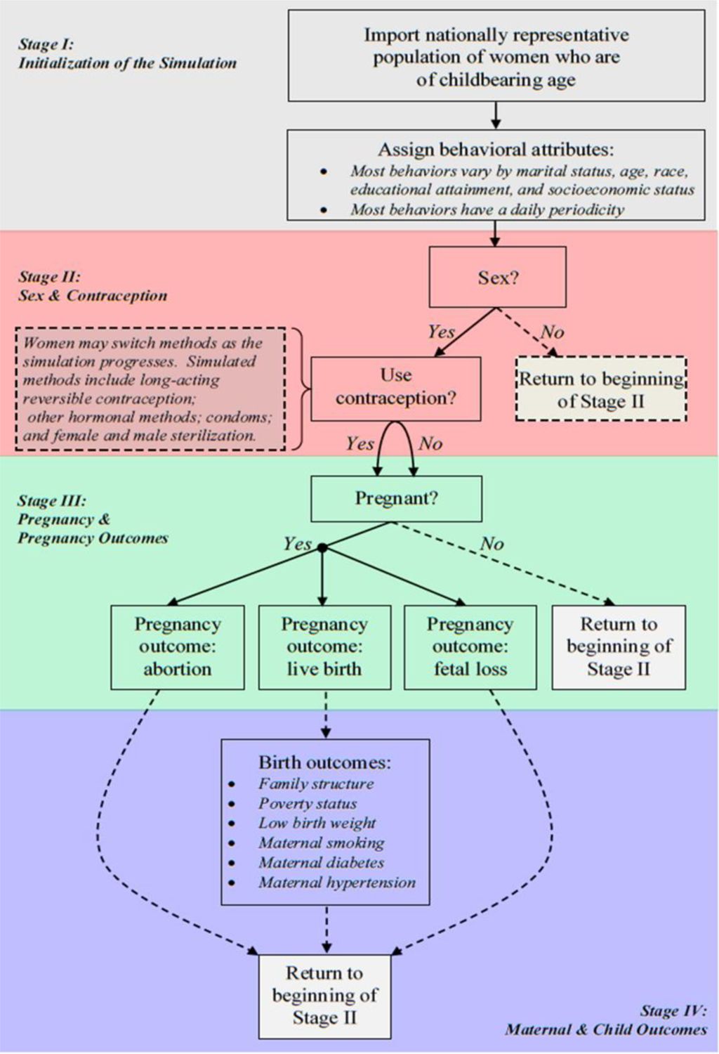
Summary diagram of the FamilyScape 3.0 microsimulation model.
2.1 Stage I: initialization of the simulation
Our simulations rely heavily on estimates derived from the 2006 – 2010 NSFG, which contains a nationally representative sample of individuals who are between 15 and 44 years of age (National Center for Health Statistics [NCHS], 2011). The NSFG collects information on respondents’ pregnancy and childbearing histories, sexual activity, contraceptive use, and a variety of other correlates of fertility, family formation, and child well-being (Lepowski, Mosher, Davis, Groves, & van Hoewyk, 2010). This survey is used extensively by scholars and practitioners to study topics related to reproductive, maternal, and infant health in the United States and by policy-makers to guide programmatic decisions with bearing on these outcomes (NCHS, 2016). The 2006 – 2010 cycle of the NSFG is a continuously fielded cross-section, which is to say that different nationally representative cross-sections are sampled in each year of the survey cycle (Lepowski et al., 2010).
While the NSFG surveys both men and women, recall that we rely exclusively on women’s responses to develop FamilyScape’s parameters. As a result, the model’s simulation population contains only women. Crucially, however, female NSFG sample members are asked for information on their use of female-controlled and male-controlled contraceptive methods. More specifically, women are asked for information on the contraceptive method or methods (female-controlled and male-controlled) that they have relied upon during each month for a period of up to four years (NCHS, 2011).8 Thus, although the NSFG is a cross-sectional survey, it provides rich retrospective data on women’s contraceptive histories. Male NSFG respondents are not asked to provide such detailed information on their past contraceptive use. As such, we would be unable realistically to model patterns of contraceptive switching for male-controlled methods if we were to rely on the self-reports of male NSFG sample members. Moreover, because reliance on men’s self-reports of contraceptive use would render us unable to model realistic patterns of male-controlled contraceptive switching, we would also be unable to condition changes in relationship formation and dissolution on the methods used by one’s (existing or potential) partner as the time passes. As previously discussed, these considerations constitute two of the primary limitations of earlier versions of the model and are the reason why men are not included in the simulation population for FamilyScape 3.0.
We would also emphasize that, while men are not included in FamilyScape’s simulation population, male behaviour is a crucial component of the model’s architecture. This is because we used women’s reports of their sexual histories with their male partners, and of the methods that their partners used, when developing the model’s sexual-activity and contraceptive-use parameters. Given that we do not explicitly simulate marital and nonmarital relationship formation and dissolution, one might argue that FamilyScape 3.0 is only a partial equilibrium model. On the other hand, relationship formation is, from the standpoint of our simulation, simply a means to an end: our ultimate goal is to model accurately the frequency of intercourse and the methods used during intercourse. As is discussed later, FamilyScape produces simulated distributions of heterosexual coital frequency, contraceptive use (at the couple level, including both male-controlled and female-controlled methods), and contraceptive switching (again, at the couple level) that are well-matched to their real-world counterparts.
We begin the simulation process by using the NSFG’s sampling weights to extract a group of 20,000 female respondents for inclusion in the simulation population.9 As we import individual observations from the NSFG into the simulation population, we retain information on each respondent’s marital status, age, race, educational attainment, and SES. We operationalize SES using a measure of maternal educational attainment (i.e., the attainment of the mothers of the members of the simulation population).10 We usually simulate variation in FamilyScape’s behavioural inputs and key outcomes according to each of these characteristics.
We considered the possibility of incorporating other covariates into the simulation, but we ultimately decided not to do so for three reasons. First, the model already contains more than a thousand input parameters, and we wanted to achieve a measure of modelling parsimony. Adding more covariates to the model would substantially increase the number of parameters that we would be required to estimate. Second, the general consensus among the experts advising us during the early stages of the FamilyScape project was that the characteristics listed above were the most important for us to include on substantive and policy grounds. And third, most of the other variables that have been found to be closely linked to family formation behaviours are time-varying. For example, contraceptive use varies according to income-to-needs status (Frost & Darroch, 2008; Jones, Mosher, & Daniels, 2012) and insurance status (Jones et al., 2012; Mosher, Jones, & Abma, 2015). Because FamilyScape is a static model, we limit our set of covariates to attributes that remain fixed over time.11 Thus, we do not include time-varying characteristics of this sort in the simulation.
Given that FamilyScape accounts for a relatively modest number of individual attributes, the regressions that estimate the model’s parameters generally have limited predictive power (see Appendix A). However, as is documented throughout this paper, FamilyScape nonetheless closely matches a multitude of important real-world benchmarks. For instance, the model realistically simulates the rate at which women have sex; the frequency with which sexually active women use contraception; the types of male-controlled and female-controlled contraceptive methods that they use; the number of women who switch onto and off of various methods; the frequency with which women using various forms of contraception (or none at all) become pregnant; the share of pregnancies that result in live births, abortions, and fatal losses; the typical gestation periods for each of these pregnancy outcomes; and the rate at which newborn children and their mothers experience a variety of adverse economic and health outcomes.
Table 1 shows the categorical specifications that were chosen for each of the demographic characteristics that are included in the simulation. We selected these specifications either based on the results of econometric analyses or because we were compelled to do so by the limitations of the data available to us.12
Specification of FamilyScape’s demographic covariates.
| Covariates | |||||
|---|---|---|---|---|---|
| Categories | Age Group | Race | Educational Attainment | SES | Marital Status |
| 15–19 | White non-Hispanic | Less than high school | Mother had less than a high school degree | Unmarried | |
| 20–24 | Black non-Hispanic | High school degree | Mother had at least a high school degree | Married | |
| 25–29 | Hispanic | More than high school | |||
| 30–44 | Other | ||||
Because we use the NSFG’s sampling weights to extract observations, the demographic characteristics of FamilyScape’s simulation population should match closely the weighted characteristics of the sample from which it was drawn. As shown in Table 2, this is in fact the case.13
Demographic comparison of the FamilyScape 3.0 simulation population and NSFG respondents.
| Simulation Population | NSFG | |
|---|---|---|
| 15–19 (%) | 16.9% | 17.1% |
| 20–24 (%) | 16.6% | 16.8% |
| 25–29 (%) | 17.6% | 17.1% |
| 30–44 (%) | 49.0% | 49.0% |
| Average age | 29.5 | 29.5 |
| White non-Hispanic (%) | 61.9% | 61.8% |
| Black non-Hispanic (%) | 14.2% | 14.4% |
| Hispanic (%) | 17.3% | 17.0% |
| Other (%) | 6.7% | 6.8% |
| Less than High School (%) | 23.7% | 24.0% |
| High School Degree (%) | 24.7% | 23.8% |
| More than High School (%) | 51.7% | 52.2% |
| Low SES (%) | 22.6% | 22.3% |
| High SES (%) | 77.4% | 77.7% |
| Unmarried (%) | 58.8% | 58.6% |
| Married (%) | 41.2% | 41.4% |
| N | 20,000 | 12,175 |
-
Sources: Simulated results were generated using data from 100 one-year steady-state runs of the FamilyScape 3.0 model. Real-world benchmarks were produced via analysis of the weighted female respondent file of the National Survey of Family Growth 2006–2010.
-
Notes: A woman is considered to be low-SES if her mother had less than a high-school degree.
At the outset of the simulation, each woman in the simulation population is assigned a set of probabilities that are subsequently used to model various aspects of her behaviour (e.g. the use of a particular contraceptive method or methods). Most of these probabilities vary as a function of women’s demographic attributes – and, in all instances in which that is true, they are derived based on the results of regression models that were estimated using real-world data. Some regressions include behavioural controls in addition to demographic covariates, as detailed below. When an individual has to make a decision about whether to take a particular action, we randomly select a number from a uniform (0,1) distribution, and the woman engages in the behaviour in question if that draw falls below the relevant probability. If a choice must be made from among more than two options, we model the relevant decision as a series of binary choices. As an example, for a choice with three options, we first model whether women choose option one (as opposed to options two or three). Among women who do not choose the first option, we then model the choice between options two and three. This approach is functionally equivalent to the modelling of simultaneous choices from among all available options, but it is easier to implement in practice.
Given FamilyScape’s heavy reliance on random variation, no two runs of the model are exactly alike. We therefore report simulation results using data that are averaged over multiple runs of the model. Our objective is to perform enough simulation runs to prevent outliers from exercising undue influence over average measures of FamilyScape’s aggregate outcomes across runs. We concluded after a series of exploratory analyses that, when the model is run about 100 distinct times, distributions of its results are consistently unimodal and roughly symmetric. Thus, all results reported in this paper are from 100 one-year simulation runs.
We would also note that no single dataset contains the breadth of information necessary to estimate the entire model’s many input parameters. Thus, once women are imported from the NSFG’s sample into the simulation population, we use data from a variety of different sources to develop the various parameters that govern their behaviour. For reasons of internal consistency, we parameterize the model using data from 2006 – 2010 whenever possible. When data from these years are not available, we use information from the closest available year. We use 2006 – 2010 data because these are the most recent years for which NSFG files were available when FamilyScape 3.0 was being developed. After we completed work on the current version of FamilyScape, a new cycle of NSFG data for 2011 – 2013 was released. However, detailed pregnancy-rate estimates have not yet been published for this recent period, which is to say that there would not be sufficient external benchmarks to allow us thoroughly to validate the model’s results if it were parameterized using this new cycle of the NSFG. Thus, the current version of FamilyScape was developed using data from the most recent time period for which the model’s results can be externally validated.
2.2 Stage II: sexual and contraceptive behaviour
The parameters for FamilyScape’s sexual behaviour modules were developed using real-world data on sexual activity across months (these data reflect the number of months over the course of a year during which a woman was sexually active) and coital frequency within months (these data reflect the number of days on which a woman had intercourse during a sexually active month).14 FamilyScape’s process for simulating sexual behaviour is thus comprised of two steps. First, we identify the months (if any) during which a given woman will be sexually active over the course of a given year of analysis time. And second, we identify the specific days on which she will have sex during a month when she is sexually active. Because the married and unmarried populations have fundamentally different distributions of coital frequency, we develop the model’s sexual behaviour parameters separately for these two groups (indeed, for almost all components of the simulation, we estimate parameters separately for married and unmarried women; as a result, we usually benchmark the model’s results separately for these two groups).
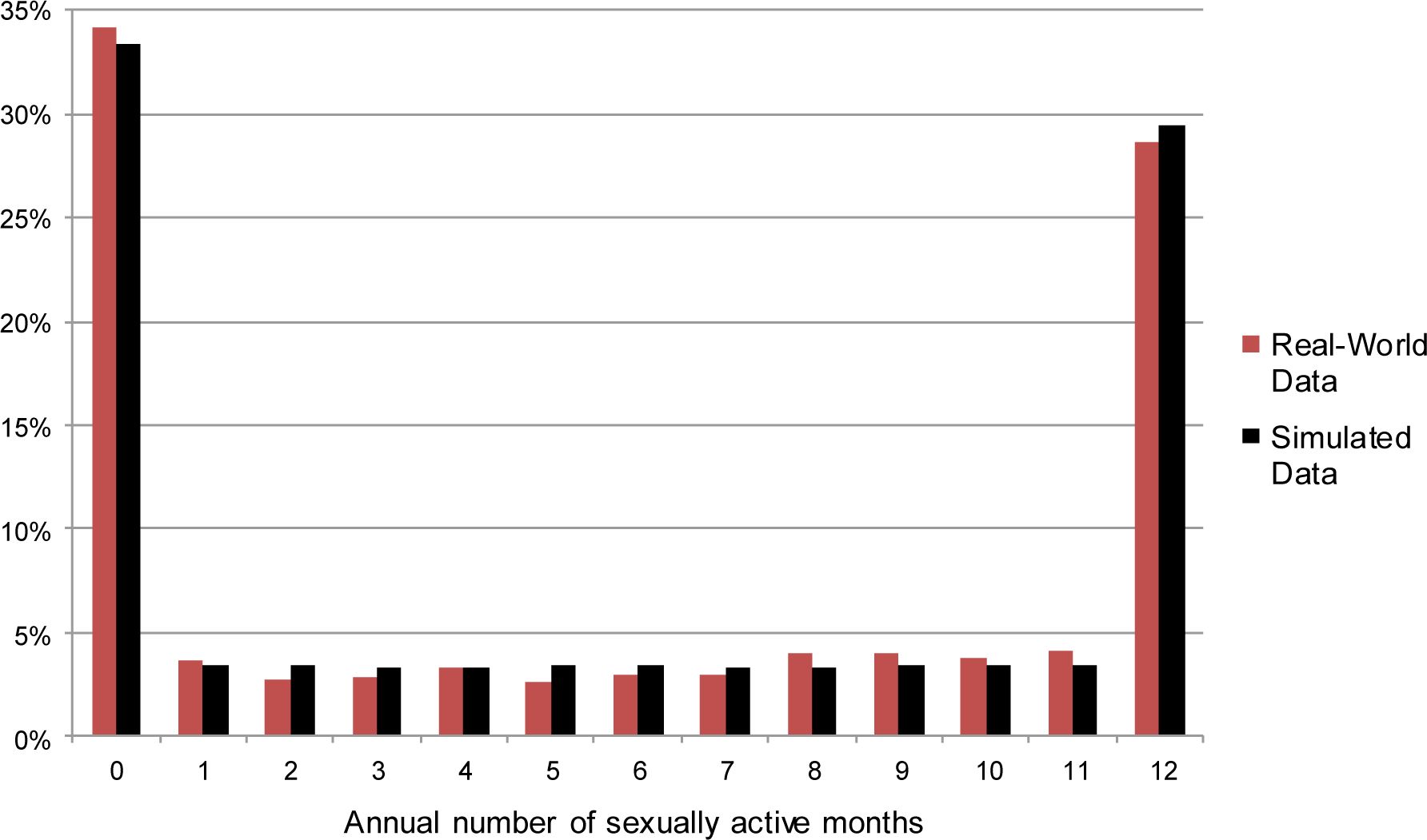
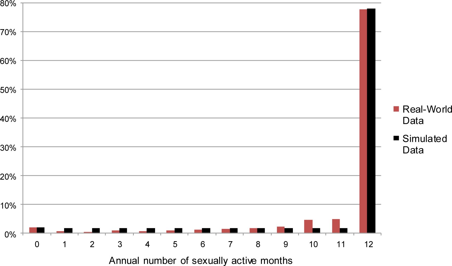
Regarding the first of the two steps described above, our analysis of data from the NSFG suggests that, over the course of a year, many women have sex at least once per month, others have no sex, and the remainder fall in between these two extremes.15 Women in the latter group are distributed relatively evenly across months. We therefore place each woman in the simulation population into one of three “annual sexual activity” categories: “highly active,” “moderately active,” or “inactive.” We use the results of analyses of the NSFG to vary women’s chances of being placed into each of these three groups as a function of their demographic characteristics. Women who are assigned to the “highly active” category are sexually active during each month of a year within the simulation; women in the “inactive” category are sexually inactive for the entire year; and women in the “moderately active” category are randomly assigned to be sexually active for between one and eleven months. Figures 2 and 3 report annual distributions of across-month sexual activity for unmarried and married women in the NSFG and in FamilyScape’s simulation population. As is shown in these figures, the simulated and real-world distributions of annual sexual activity are qualitatively similar to one another.

Simulated and real-world annual number of sexually active months, among unmarried women.
Sources: Simulated results were generated using data from 100 one-year steady-state runs of the FamilyScape 3.0 model. Real-world estimates were produced via tabulations of data taken from the female respondent file of the 2006 – 2010 National Survey of Family Growth.
Notes: We do not display confidence intervals because they are so small as to be invisible to the naked eye.

Simulated and real-world annual number of sexually active months, among married women.
Sources: Simulated results were generated using data from 100 one-year steady-state runs of the FamilyScape 3.0 model. Real-world estimates were produced via tabulations of data taken from the female respondent file of the 2006 – 2010 National Survey of Family Growth.
Notes: We do not display confidence intervals because they are so small as to be invisible to the naked eye.
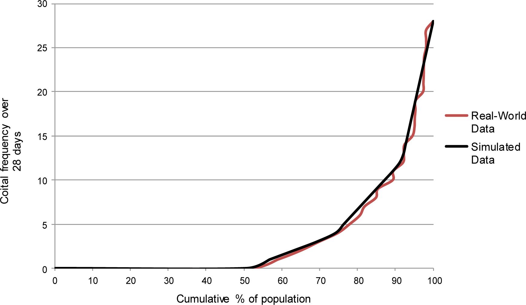
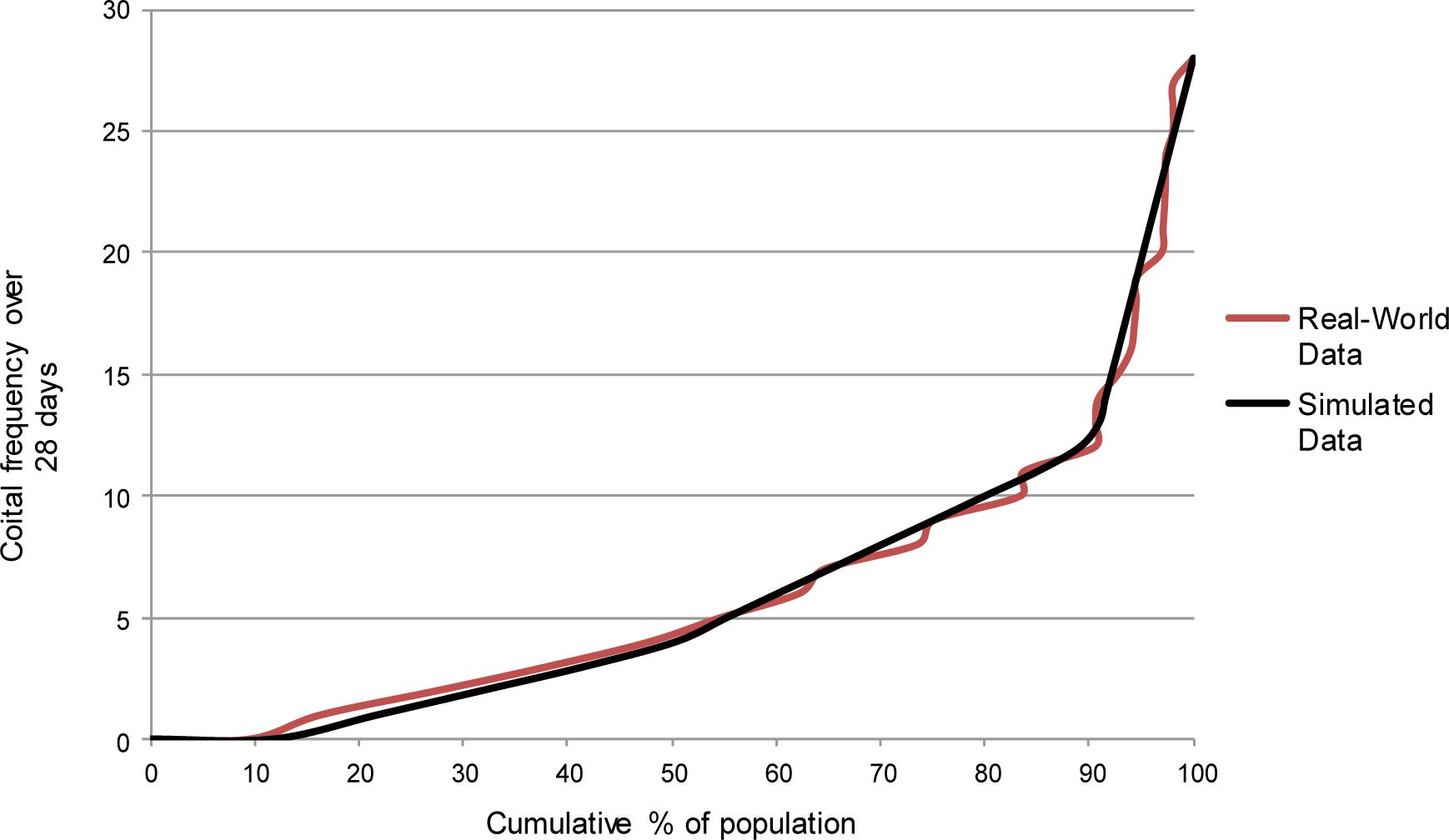
Among women in the NSFG who are sexually active during a given month, the within-month distribution of coital frequency is similar to the above-described distribution of sexual activity across months. In other words, sexually active women can readily be grouped into “high,” “moderate,” and “low” categories with respect to their within-month coital frequency. In order to develop the model’s parameters governing coital frequency during a sexually active month, we therefore use NSFG-derived parameters to assign women to one of three different groups, again as a function of their demographic characteristics.16 We also vary a woman’s chances of falling into each of these groups as a function of her annual sexual activity type. We then calibrate the model to ensure that: a) women in the “high” coital-frequency category have intercourse more often than women in the “moderate” coital-frequency category; b) women in the “moderate” coital-frequency category have intercourse more often than women in the “low” coital-frequency category; and c) the simulation produces a realistic distribution of overall within-month coital frequency. Figure 4 compares the cumulative distribution of within-month coital frequency among unmarried NSFG respondents with the equivalent distribution from a series of FamilyScape simulation runs. Figure 5 shows the same comparison for married women.17 These figures include data on women who have no sex during a given month as a means of further validating the model’s capacity to simulate sexual inactivity. For both groups, the simulated and real-world distributions of within-month coital frequency are quite comparable.
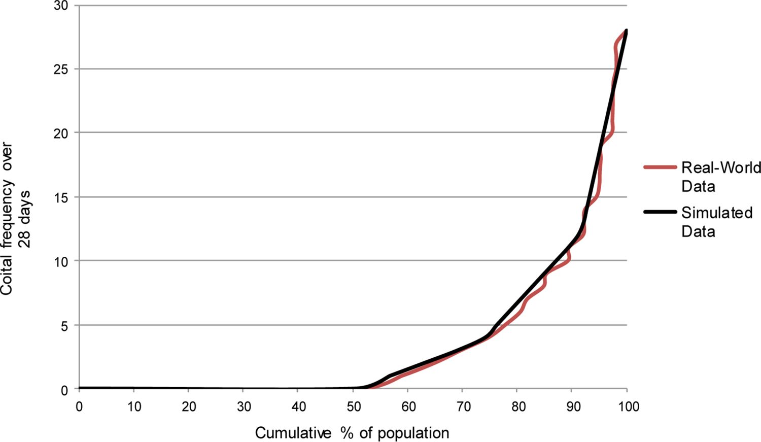
Simulated and real-world within-month coital frequency distributions, among unmarried women.
Sources: Simulated results were generated using data from 100 one-year steady-state runs of the FamilyScape 3.0 model. Real-world estimates were produced via tabulations of data taken from the female respondent file of the 2006 – 2010 National Survey of Family Growth.
Notes: We do not display confidence intervals because they are so small as to be invisible to the naked eye.

Simulated and real-world within-month coital frequency distributions, among married women.
Sources: Simulated results were generated using data from 100 one-year steady-state runs of the FamilyScape 3.0 model. Real-world estimates were produced via tabulations of data taken from the female respondent file of the 2006 – 2010 National Survey of Family Growth.
Notes: We do not display confidence intervals because they are so small as to be invisible to the naked eye.
We now describe the model’s procedures for simulating contraceptive behaviour. At the start of a simulation run, members of FamilyScape’s simulation population are assigned to the use of a particular female-controlled and/or male-controlled method (or to the use of no method at all) according to their demographic and behavioural characteristics. We assign women to initial contraceptive categories using data on method use among female NSFG respondents. More specifically, we use contraceptive calendar data on method use during the first month of the past year in which NSFG respondents report that they were sexually active and were not pregnant (we also allow women to switch methods over the course of the simulation using an approach detailed below).
With respect to female-controlled methods, we simulate the use of three different categories of contraception: long-acting reversible contraceptive methods (LARC); other hormonal methods such as the pill, patch, or ring (PPR); and female sterilization.18 With respect to male-controlled methods, we simulate the use of condoms and male sterilization.19 We also allow for the possibility that a woman will not use any female- or male-controlled methods. Indeed, a nontrivial number of women are noncontraceptors in the NSFG, and therefore also within FamilyScape’s simulation population. For contraceptive categories that contain several different methods, FamilyScape’s estimates of contraceptive efficacy represent a weighted average of the relevant methods’ efficacies. Because we use women’s self-reports on their own (female-controlled) methods and their partners’ (male-controlled) methods, we are able to model dual-method use at the couple level. In other words, some women are assigned to the use of PPR methods and condoms; others are assigned to use LARC methods and no male-controlled method; others are assigned to use condoms and no female-controlled method; and so forth.
As we do for sexual behaviour, we use the results of NSFG-based regressions to vary women’s chances of assuming a given contraceptive type according to their demographic characteristics. We also vary contraceptive choice as a function of annual sexual activity type and within-month coital frequency type. Thus, if women who report having relatively more (or less) intercourse in our real-world data also report being relatively more (or less) likely to use a particular type of contraception (or not to use any contraception at all), that dynamic is captured in our estimation of this module’s parameters. Table 3 compares distributions of initial contraceptive method use among female NSFG respondents and members of FamilyScape’s simulation population. The estimates reported in this table reflect the choice of methods among women who are sexually active and are not pregnant. These results confirm that FamilyScape produces distributions of couple-level contraceptive use that are closely matched to the relevant benchmarks from the NSFG.
Simulated and real-world distributions of initial contraceptive type, by marital status.
| Female-Controlled Method (if any) | Male-Controlled Method (if any) | unmarried Women | Married Women |
|---|---|---|---|
| Simulated Data | |||
| None | None | 12.6% (12.5%-12.7%) | 15.5% (15.4%-15.6%) |
| None | Condom | 31.9% (31.8%-32.0%) | 19.4% (19.3%-19.5%) |
| PPR | Nothing | 19.7% (19.6%-19.8%) | 19.8% (19.7%-19.9%) |
| PPR | Condom | 13.9% (13.8%-14.0%) | 3.9% (3.9%-3.9%) |
| LARC | Nothing | 5.6% (5.6%-5.6%) | 6.6% (6.5%-6.7%) |
| LARC | Condom | 1.7% (1.7%-1.7%) | 0.3% (0.3%-0.3%) |
| Any Method Other Than Sterilization | Sterilization | 2.1% (2.1%-2.1%) | 11.7% (11.6%-11.8%) |
| Sterilization | Any Method | 12.6% (12.5%-12.7%) | 22.8% (22.7%-22.9%) |
| Total | 100% | 100% | |
| Real-World Data | |||
| None | None | 11.6% | 15.1% |
| None | Condom | 32.1% | 19.2% |
| PPR | Nothing | 19.4% | 20.0% |
| PPR | Condom | 13.5% | 3.9% |
| LARC | Nothing | 5.9% | 6.7% |
| LARC | Condom | 1.6% | 0.3% |
| Any Method Other Than Sterilization | Sterilization | 2.6% | 11.9% |
| Sterilization | Any Method | 13.3% | 22.9% |
| Total | 100.0% | 100.0% | |
-
Sources: Simulated results were generated using data from 100 one-year steady-state runs of the FamilyScape 3.0 model. Real-world estimates were produced via tabulations of data taken from the National Survey of Family Growth (NSFG) 2006–2010.
-
Notes: Ninety-five percent confidence intervals are reported in parentheses beneath each simulated estimate. Confidence intervals reflect uncertainty related to random variation in simulation results across runs. Simulated estimates indicate initial contraceptive assignment among members of FamilyScape's simulation population. Real-world estimates indicate the most effective couple-level method(s) used in the first sexually active month of the past year among female NSFG respondents.
As the simulation progresses, noncontracepting women are allowed to begin using contraception, and contracepting women are allowed to discontinue contraceptive use or to switch methods.20 Women are allowed to begin (or to discontinue) the use of both female- and male-controlled methods. Because FamilyScape’s simulation population functions as a fixed cohort, and since some demographic groups in the real world (and therefore also in the simulation) are more likely than others to adopt certain switching patterns, different contraceptive categories would ultimately become absorbing states for different demographic groups if we were to allow the model to run in perpetuity after the contraceptive switching module was activated. Over the course of a single simulated year, however, such changes mirror realistic developments in female contraceptive behaviours within the simulation population. For this reason, we only activate FamilyScape’s contraceptive switching module for a single year of analysis time. More precisely, we first allow all other behaviours and outcomes (e.g., sexual activity, pregnancy, and childbearing) to reach steady states, and we then allow contraceptive switching to occur over a 365-day window during which we also record data on all simulation outputs of interest (e.g., births, abortions, etc.). All of our reported simulation results reflect outcomes as measured over this one-year period of analysis time.
Contraceptive switching is simulated on a monthly basis. Women are allowed to change contraceptive types multiple times over the course of a year, but they are only considered to be eligible for method switching during months in which they are sexually active and not pregnant. It is also important to note that many women in the real world (and therefore also in the simulation population) do not switch contraceptive types at all: a large share of women using LARC methods will continue to do so throughout the year; many noncontraceptors will not begin using contraception; and so forth.
FamilyScape’s switching module is parameterized using results from four different sets of regression models, each of which is estimated using the 2006 – 2010 NSFG: a) discrete-time hazard models predicting the probability that a woman will switch methods for the first time during a given twelve-month segment; b) hazard models predicting the probability of a “higher-order” contraceptive switch among women who have already switched methods at least once during the twelve-month segment; c) logistic regressions that predict the contraceptive type assumed by a woman who switches methods for the first time; and d) logistic regressions that predict the contraceptive type assumed by a woman who has engaged in a higher-order method switch. Switching probabilities and method selection after a switch vary according to a woman’s demographic attributes, the contraceptive method(s, or lack thereof) that she had previously been using, and whether she was pregnant in the previous month. Higher-order switching behaviours also vary according to the number of previous contraceptive switches.
Tables 4 and 5 allow for an assessment of FamilyScape’s ability to simulate realistic switching behaviours. Both tables report, for women in each origin contraceptive category, the across-month distribution of method choice over a period of twelve months starting with the month in which the origin method was identified. Real-world benchmarks were estimated using the NSFG, and simulated estimates were produced using microdata taken from the year of analysis time during which the model’s switching module was activated. Table 4 reports switching estimates for unmarried women, and Table 5 reports the same for married women. For instance, the second row of data in each panel of Table 4 reports estimates of switching behaviours among unmarried women whose origin contraceptive type was “No Female-Controlled Method & Condom.” Within the simulation, women in this origin category spend an average of 3.9% of months during the focal year in the “No Female-Controlled Method & No Male-Controlled Method” category. The corresponding estimate is 3.6% for our NSFG sample. More broadly, the results reported in these tables demonstrate that FamilyScape’s simulated switching patterns are generally analogous to their real-world equivalents.21
Simulated and real-world contraceptive switching distributions, among unmarried women.
| Origin Contraceptive Type | Contraceptive-Type Distribution Across Twelve Consecutive Months | ||||||||
|---|---|---|---|---|---|---|---|---|---|
| Female-Controlled Method | Male-Controlled Method | Female Method: Nothing Male Method: Nothing | Female Method: Nothing Male Method: Condom | Female Method: PPR Male Method: Nothing | Female Method: PPR Male Method: Condom | Female Method: LARC Male Method: Nothing | Female Method: LARC Male Method: Condom | Female Method: Anything But Sterilization Male Method: Sterilization | Female Method: Sterilization Male Method: Any Method |
| Simulated Data | |||||||||
| None | None | 88.2% (88.0%–88.3%) | 4.5% (4.4%–4.6%) | 2.6% (2.5%–2.7%) | 0.6% (0.6%–0.7%) | 2.0% (1.9%–2.0%) | 0.1% (0.0%–0.1%) | 0.2% (0.2%–0.3%) | 1.8% (1.8%–1.9%) |
| None | Condom | 3.9% (3.8%–3.9%) | 87.9% (87.8%–88.0%) | 3.2% (3.1%–3.2%) | 2.7% (2.7%–2.8%) | 1.0% (1.0%–1.1%) | 0.3% (0.2%–0.3%) | 0.5% (0.5%–0.5%) | 0.5% (0.5%–0.6%) |
| PPR | None | 2.7% (2.6%–2.7%) | 3.3% (3.2%–3.4%) | 88.8% (88.7%–88.9%) | 3.1% (3.0%–3.1%) | 1.2% (1.1%–1.2%) | 0.1% (0.1%–0.1%) | 0.3% (0.3%–0.3%) | 0.6% (0.5%–0.6%) |
| PPR | Condom | 1.7% (1.6%–1.8%) | 4.2% (4.1%–4.3%) | 6.9% (6.8%–7.0'%) | 85.8% (85.7%–86.0%) | 0.5% (0.5%–0.5%) | 0.4% (0.4%–0.5%) | 0.3% (0.2%–0.3%) | 0.2% (0.2%–0.2%) |
| LARC | None | 4.1% (4.0%–4.3%) | 3.5% (3.3%–3.7%) | 4.6% (4.4%–4.8%) | 0.6% (0.5%–0.6%) | 84.5% (84.2%–84.9%) | 1.4% (1.3%–1.5%) | 0.2% (0.2%–0.3%) | 1.0% (0.9%–1.1%) |
| LARC | Condom | 1.4% (1.3%–1.6%) | 7.2% (6.9%–7.6%) | 2.1% (1.9%–2.3%) | 2.6% (2.3%–2.8%) | 6.0% (5.6%–6.3%) | 79.6% (79.1%–80.2%) | 0.1% (0.1%–0.2%) | 0.9% (0.8%–1.1%) |
| Any Method Other Than Sterilization | Sterilization | 1.6% (1.5%–1.8%) | 3.3% (3. 1 %–3.5 %) | 0.8% (0.7%–0.9%) | 0.5% (0.4%–0.6%) | 0.5% (0.5%–0.6%) | 0.2% (0.1%–0.2%) | 92.3% (92.0%–92.6%) | 0.8% (0.7%–0.9%) |
| Sterilization | Any Method | 0.0% (0.0%–0.0%) | 0.0% (0.0%–0.0%) | 0.0% (0.0%–0.0%) | 0.0% (0.0%–0.0%) | 0.0% (0.0%–0.0%) | 0.0% (0.0%–0.0%) | 0.0% (0.0%–0.0%) | 100% (100.0%–100.0%) |
| Real-World Data | |||||||||
| None | None | 84.9% | 5.9% | 3.6% | 1.2% | 2.4% | 0.3% | 0.6% | 1.1% |
| None | Condom | 3.6% | 88.4% | 3.1% | 3.3% | 0.7% | 0.2% | 0.4% | 0.3% |
| PPR | None | 4.0% | 4.9% | 86.8% | 2.8% | 1.0% | 0.0% | 0.2% | 0.3% |
| PPR | Condom | 1.3% | 4.8% | 8.1% | 84.8% | 0.3% | 0.5% | 0.1% | 0.1% |
| LARC | None | 5.3% | 3.7% | 4.8% | 0.8% | 83.5% | 1.2% | 0.0% | 0.6% |
| LARC | Condom | 0.9% | 8.3% | 1.0% | 3.0% | 5.2% | 81.3% | 0.1% | 0.3% |
| Any Method Other Than Sterilization | Sterilization | 0.6% | 3.5% | 0.7% | 1.6% | 0.1% | 0.0% | 92.9% | 0.6% |
| Sterilization | Any Method | 0.5% | 0.1% | 0.2% | 0.1% | 0.1% | 0.1% | 0.0% | 99.0% |
-
Sources: Simulated results were generated using data from 100 one-year steady-state runs of the FamilyScape 3.0 model. Real-world estimates were produced using data on female members of the National Survey of Family Growth 2006–2010.
-
Notes: Ninety-five percent confidence intervals are reported in parentheses beneath each simulated estimate. Confidence intervals reflect uncertainty related to random variation in simulation results across runs.
Simulated and real-world contraceptive switching distributions, among married women.
| Origin Contraceptive Type | Contraceptive-Type Distribution Across Twelve Consecutive Months | ||||||||
|---|---|---|---|---|---|---|---|---|---|
| Female-Controlled Method | Male-Controlled Method | Female Method: Nothing Male Method: Nothing | Female Method: Nothing Male Method: Condom | Female Method: PPR Male Method: Nothing | Female Method: PPR Male Method: Condom | Female Method: LARC Male Method: Nothing | Female Method: LARC Male Method: Condom | Female Method: Anything But Sterilization Male Method: Sterilization | Female Method: Sterilization Male Method: Any Method |
| Simulated Data | |||||||||
| None | None | 90.6% (90.4%–90.7%) | 2.6% (2.5%–2.6%) | 3.5% (3.4%–3.6%) | 0.3% (0.3%–0.3%) | 1.0% (0.9%–1.0%) | 0.0% (0.0%–0.0%) | 0.7% (0.7%–0.8%) | 1.3% (1.3%–1.4%) |
| None | Condom | 4.3% (4.2%4.4%) | 90.3% (90.2%–90.4%) | 1.8% (1. 7%–1 8%) | 0.5% (0.5%–0.6%) | 0.8% (0.8%–0.9%) | 0.1% (0.1%–0.1%) | 1.2% (1.2%–1.3%) | 0.9% (0.9%–1.0%) |
| PPR | None | 5.3% (5.2%–5.4%) | 3.2% (3.2%–3.3%) | 87.6% (87.5%–87.7%) | 1.2% (1.2%–1.2%) | 0.9% (0.9%–1.0%) | 0.1% (0.1%–0.1%) | 1.0% (0.9%–1.0%) | 0.6% (0.6%–0.6%) |
| PPR | Condom | 3.1% (2.9%–3.3%) | 5.9% (5.7%–6.2%) | 4.5% (4.3%–4.7%) | 84.4% (84.0%–84.7%) | 0.7% (0.6%–0.7%) | 0.1% (0.1%–0.1%) | 1.0% (0.9%–1.0%) | 0.3% (0.3%–0.4%) |
| LARC | None | 1.9% (1.8%–2.0%) | 1.9% (1.8%–1.9%) | 2.2% (2.1%–2.3%) | 0.2% (0.2%–0.3%) | 92.3% (92.1%–92.5%) | 0.2% (0.2%–0.2%) | 0.6% (0.5%–0.6%) | 0.7% (0.7%–0.8%) |
| LARC | Condom | 0.9% (0.6%–1.2%) | 7.2% (6.4%–8.0%) | 0.7% (0.5%–0.9%) | 0.8% (0.6%–1.0%) | 9.5% (8.5 %–10.5 %) | 79.9% (78.5 %–81.3 %) | 0.1% (0.0%–0.3%) | 0.9% (0.7%–1.1%) |
| Any Method Other Than Sterilization | Sterilization | 0.0% (0.0%–0.0%) | 0.0% (0.0%–0.0%) | 0.0% (0.0%–0.0%) | 0.0% (0.0%–0.0%) | 0.0% (0.0%–0.0%) | 0.0% (0.0%–0.0%) | 100% (100.0%–100.0%) | 0.0% (0.0%–0.0%) |
| Sterilization | Any Method | 0.0% (0.0%–0.0%) | 0.0% (0.0%–0.0%) | 0.0% (0.0%–0.0%) | 0.0% (0.0%–0.0%) | 0.0% (0.0%–0.0%) | 0.0% (0.0%–0.0%) | 0.0% (0.0%–0.0%) | 100% (100.0%–100.0%) |
| Real-World Data | |||||||||
| None | None | 88.2% | 3.6% | 4.3% | 0.4% | 1.2% | 0.0% | 0.9% | 1.3% |
| None | Condom | 4.3% | 90.1% | 1.4% | 0.9% | 1.1% | 0.1% | 1.6% | 0.5% |
| PPR | None | 6.8% | 3.5% | 86.5% | 0.7% | 0.8% | 0.0% | 1.2% | 0.6% |
| PPR | Condom | 2.8% | 2.8% | 5.4% | 87.3% | 0.5% | 0.2% | 1.0% | 0.0% |
| LARC | None | 3.2% | 1.8% | 2.6% | 0.2% | 91.2% | 0.1% | 0.6% | 0.4% |
| LARC | Condom | 0.1% | 0.8% | 0.0% | 0.0% | 11.8% | 87.2% | 0.0% | 0.0% |
| Any Method Other Than Sterilization | Sterilization | 0.4% | 0.0% | 0.1% | 0.0% | 0.0% | 0.0% | 98.7% | 0.8% |
| Sterilization | Any Method | 0.2% | 0.1% | 0.0% | 0.0% | 0.0% | 0.0% | 0.1% | 99.5% |
-
Sources: Simulated results were generated using data from 100 one-year steady-state runs of the FamilyScape 3.0 model. Real-world estimates were produced using data on female members of the National Survey of Family Growth 2006–2010.
-
Notes: Ninety-five percent confidence intervals are reported in parentheses beneath each simulated estimate. Confidence intervals reflect uncertainty related to random variation in simulation results across runs.
The reader should bear in mind that, within the context of FamilyScape’s architecture, the concept of contraceptive consistency is distinct from the concept of contraceptive switching. As an example, a woman who is considered to be a pill user during every month of a given year (i.e., a woman who does not switch methods over the course of the year) might also be an inconsistent contraceptor (if she misses a certain number of pills per month). In order directly to simulate inconsistency of contraceptive use, we would require two pieces of information that we do not have. First, we would need data on the distribution of the consistency of method use. For instance, we would require information on the proportion of oral contraceptors who miss one pill per month, the proportion who miss two pills per month, and so forth. And second, we would require evidence on the relationship between each method’s efficacy and the consistency with which it is used. For example, we would require information on the decline in the efficacy of oral contraception when one pill is missed, the further decline in efficacy when two pills are missed, and so forth. We would require similar information in order to simulate variation in the correctness of contraceptive use (i.e., the extent to which methods such as condoms are used as intended).
Such data do not exist. We have therefore chosen not to attempt directly to integrate these dynamics into FamilyScape. Rather, we capture much of the variation in the consistency and correctness of contraceptive use by allowing the efficacies of the methods incorporated into the simulation to vary across demographic groups. There are in fact substantial demographic differences in many methods’ efficacy levels. Much of this variation occurs across marital-status and age categories. For instance, we estimate that the single-act contraceptive failure rate for PPR methods is about 35% lower among married women over the age of 30 than among unmarried women under 30. We assume that this sort of variation reflects demographic differences in the consistency and correctness of method use among women who fall into different contraceptive categories. Under this assumption, FamilyScape accounts for a portion of the heterogeneity that exists in the consistency and correctness with which various methods are used. FamilyScape’s contraceptive efficacy module is described in more detail in the next subsection.
2.3 Stage III: pregnancy and pregnancy outcomes
As is the case in the real world, a woman’s chance of becoming pregnant after having sex during the simulation depends on her level of fecundity (i.e., her probability of conceiving from a single act of unprotected intercourse) and on the effectiveness of the contraceptive method(s, if any) that she and her partner using. FamilyScape allows for variation in a woman’s fecundity as a function of her age and the day in her menstrual cycle. Thus, as the simulation advances from one day to the next, it also updates each woman’s menstrual calendar and modifies her (age-adjusted) fecundity level accordingly. We assign age-and-day-specific fecundity values based on our synthesis of the results of several published clinical studies. We rely primarily on Royston’s (1982) results for this purpose because his model has the unique benefit of allowing the probability of pregnancy to vary simultaneously as a function of the woman’s age and her menstrual calendar. Royston estimates parameters for the following equation:
where P(conception)i,t is the probability that individual i will conceive if she has unprotected sex on day t; Ai is the age of individual i; Ā is the mean age of all of the women in the author’s sample; χ0 and χ1 are econometrically estimated parameters that capture the age-dependent likelihood of fertilization; and αt is a vector of generic probabilities of ovular fertilization that vary by the day in the menstrual cycle.22 Royston derived his estimates using data on a sample of women aged 20–39 (Barrett & Marshall, 1969; Royston, 1982). However, given that the women in FamilyScape’s simulation population are between the ages 15 and 44, we use the results of a number of other clinical studies to adjust the imputed fecundity levels assigned to women in the tails of FamilyScape’s age distribution (Dunson, Colombo, & Baird, 2002; Lass et al., 1998; Leridon, 2004).23
As previously discussed, we simulate variation in the consistency and correctness of contraceptive use by modelling variation across demographic groups in the risk of pregnancy that is associated with the use of a given method.24 We calculate a method’s failure rate as follows. Assume that a woman’s fecundity level is given by the constant f, and assume that she has intercourse n times over a one-year period. Thus, the woman’s probability of avoiding pregnancy from a single act of intercourse is (1-f), her probability of avoiding pregnancy over n acts of intercourse can be assumed to be (1-f)n, and her risk of experiencing a pregnancy over n acts of intercourse is (1 – (1-f)n). Now assume that the woman in question uses a contraceptive method that reduces her risk of pregnancy by 95% each time she has sex. We define this method’s “single-act failure rate” to be (1-.95) = .05. According to this formulation, the woman’s single-act conception probability is now .05*f, and her conception probability over n acts of intercourse is (1 – (1-(.05*f))n).
More generally, one can think of a method’s single-act failure rate, c, as one minus its “efficacy rate”, where contraceptive efficacy in this context is defined as the proportional reduction in the risk of pregnancy at a given act of intercourse that is achieved by the use of that method. Although we allow for demographic variation in most methods’ single-act failure rates, we make the simplifying assumption that failure rates are homogenous within groups. Our approach thus yields the following generalized equation:
where P(Pregnant)i,j is the monthly probability of experiencing a pregnancy for women who are in demographic subgroup i and are using method j; fi,j gives the mean fecundity level (averaged across all relevant ages and all days in the menstrual cycle) for women in demographic group i who use method j; ni,j gives the average monthly coital frequency among women in demographic group i who use method j; and ci,j gives the contraceptive failure rate experienced by women in demographic group i who use method j. We then re-state Equation 2 as follows in order to solve for ci,j
We perform separate calculations for each distinct combination of i and j. In other words, we develop demographically specific single-act failure-rate estimates for each possible combination of female- and male-controlled methods. For example, we separately calculate dual-method failure rates for women who use a PPR method and condoms and single-method failure rates for women who use a PPR method and no male-controlled method. The only exception to this rule is sterilization: we make the simplifying assumption that the risk of pregnancy is completely eliminated for any woman who is sterilized or whose partner is sterilized.
We estimate ni,j using data on the monthly coital frequencies of women in the 2006 – 2010 NSFG who fall into each demographic-contraceptive-method subgroup. We produce demographically specific estimates of fi,j, by: a) using our adjusted Royston equations to calculate a single fecundity estimate, averaged across all days in the menstrual cycle, for each woman in the NSFG; and b) using these estimates to calculate a mean fecundity level for each demographic-contraceptive-method group. We estimate P(Pregnant)i,j in two stages. First, we use the NSFG to estimate the monthly pregnancy rates of women falling into each demographic subgroup. And second, because abortions have been found to be substantially underreported in the NSFG (Jones & Kost, 2007), we correct our NSFG-based estimates of method-specific pregnancy rates for abortion underreporting. Our corrections rely on data taken from Jones, Darroch, and Henshaw (2002) and Jones and Jerman (2014).25 After developing demographically specific estimates of ni,j, fi,j, and P(Pregnant)i,j, we plug these quantities into Equation 3 in order to calculate a single-act contraceptive failure rate for each demographic-contraceptive-method subgroup. We then calculate a woman’s single-act conception probability at a given act of intercourse by taking the product of her (day-and-age-specific) natural fecundity level and the single-act failure rate of the contraceptive method(s, if any) that she is using.
Having described the way in which FamilyScape simulates the occurrence of pregnancy, we next benchmark the model’s simulated annual contraceptive failure rates among women who use various forms of birth control. The best available real-world estimates of method-specific pregnancy rates are reported by Trussell (2011), who calculates the probability of experiencing a pregnancy within a year of typical use of a given method. We calculate weighted averages of these method-specific pregnancy probabilities in order to produce estimates for broad contraceptive groupings that are comparable to FamilyScape’s contraceptive categories. The weights used in these calculations reflect the relative shares of women who use each method included within a given contraceptive category. We employ contraceptive-use data reported in Jones et al. (2012) to develop these weights.
Table 6 compares FamilyScape’s simulated method-specific annual pregnancy probabilities to our real-world benchmarks. Because Trussell’s estimates are not disaggregated by marital status (or by any other demographic characteristic), we report simulated method-specific pregnancy rates for all women, without respect to marital status. Note that we report simulated and real-world estimates for women not using any contraception. There is wide variation in real-world estimates of risk of pregnancy among noncontraceptors. For example, Trussell (2011) concludes that women currently using reversible contraception would have an 85% probability of becoming pregnant if they were to discontinue use of their methods but leave their behaviour otherwise unchanged. However, other research suggests that the annual pregnancy rate is 46% among women who abandon contraception and are not seeking pregnancy (Vaughan, Trussell, Kost, & Jones, 2008). Thus, we report a range of 46% to 85% as the real-world benchmark for the “no-method” group. For male and female sterilization, LARC methods, PPR methods, and condoms, the simulated and real-world estimates reported in Table 6 are very similar to each other. The simulated annual pregnancy probability for women in the “no-method” group is roughly equidistant of the two real-world benchmarks for this category. In sum, FamilyScape closely approximates annual real-world, method-specific contraceptive failure rates.
Simulated and real-world estimates of the proportion of women experiencing a pregnancy within a year of typical use, by contraceptive method.
| Simulated Data | Real-World Data | |
|---|---|---|
| No Method | 66.7% (66.5%–66.9%) | Between 46.0% and 85.0% |
| Condoms | 20.2% (20.1%–20.3%) | 19.0% |
| PPR | 9.6% (9.5%–9.7%) | 9.7% |
| LARC | 3.1% (3.0%–3.2%) | 2.7% |
| Male Sterilization | 0.0% (0.0%–0.0%) | .15% |
| Female Sterilization | 0.0% (0.0%–0.0%) | .5% |
-
Sources: Simulated results were generated using data from 100 one-year steady-state runs of the FamilyScape 3.0 model. Real-world estimates were produced using data taken from Trussell (2011) and Jones et al. (2012).
-
Notes: Ninety-five percent confidence intervals are reported in parentheses beneath each simulated estimate. Confidence intervals reflect uncertainty related to random variation in simulation results across runs.
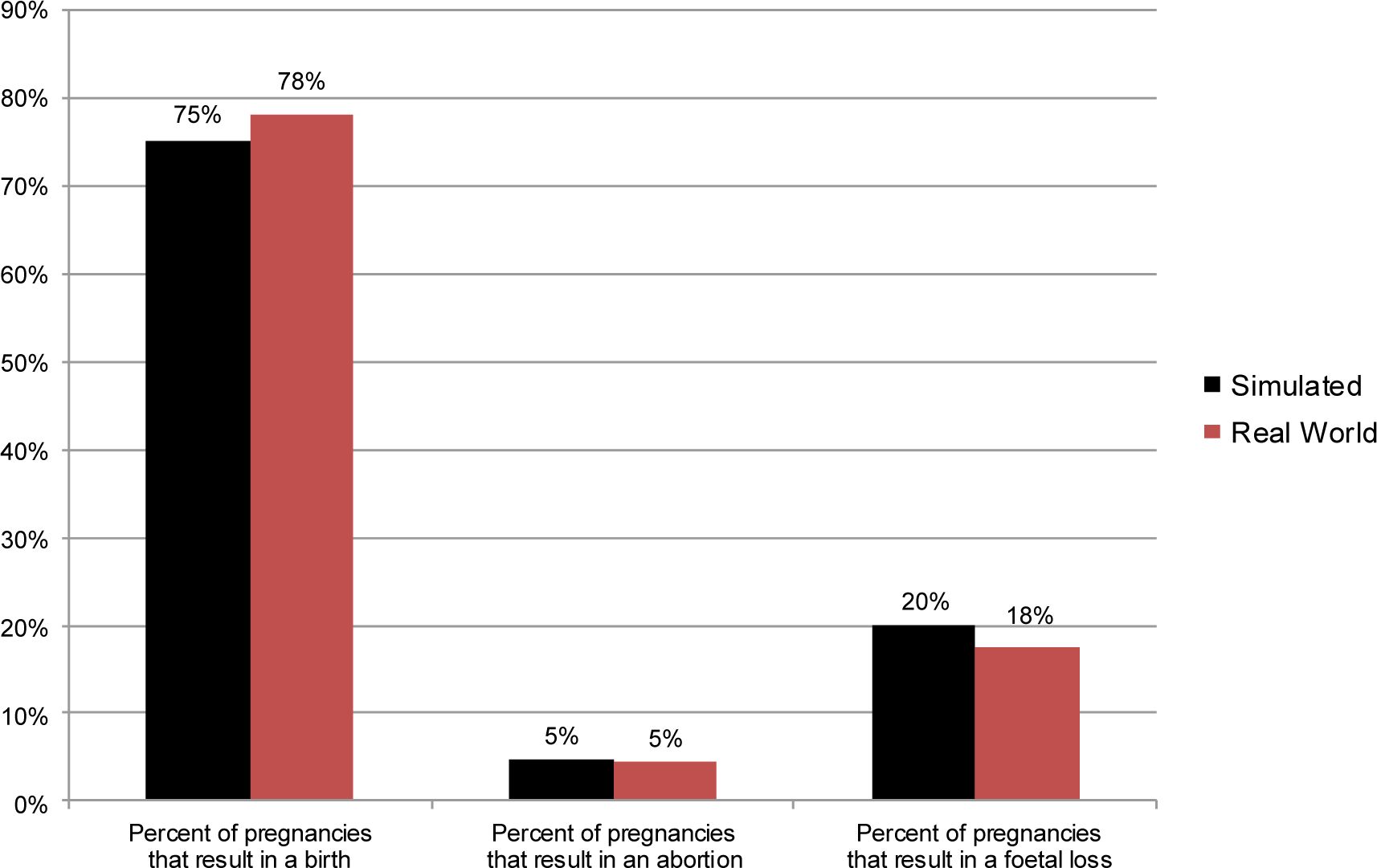
After a woman in the simulation becomes pregnant, her simulated pregnancy will eventually result in a live birth, an abortion, or a fatal loss. We use information from the National Center for Health Statistics’ 2008 National Vital Statistics System (NVSS), the Guttmacher Institute’s 2008 Abortion Provider Survey, and the 2006 – 2010 NSFG to assign an outcome to each new pregnancy as a function of the woman’s demographic characteristics.26 Figure 6 compares simulated and real-world data on the shares of pregnancies to unmarried women that result in live births, induced abortions, and fatal losses. Figure 7 presents the same comparison for pregnancies to married women. For both groups, FamilyScape produces realistic pregnancy-outcome distributions.

Simulated and real-world pregnancy outcome distributions, among unmarried women.
Sources: Simulated results were generated using data from 100 one-year steady-state runs of the FamilyScape 3.0 model. Real-world estimates were produced via tabulations of data taken from the 2006 – 2010 National Survey of Family Growth and the Guttmacher Institute’s 2008 Abortion Provider Survey.
Notes: We do not display confidence intervals because they are so small as to be invisible to the naked eye.

Simulated and real-world pregnancy outcome distributions, among married women.
Sources: Simulated results were generated using data from 100 one-year steady-state runs of the FamilyScape 3.0 model. Real-world estimates were produced via tabulations of data taken from the 2006 – 2010 National Survey of Family Growth and the Guttmacher Institute’s 2008 Abortion Provider Survey.
Notes: We do not display confidence intervals because they are so small as to be invisible to the naked eye.
Although a woman within the simulation may continue to have sex while she is pregnant, she cannot become pregnant again for the duration of her pregnancy or during an interval of simulated post-pregnancy infertility. We synthesize information from several different sources to develop the model’s parameters governing the lengths of the gestation periods and post-pregnancy infertility intervals for each pregnancy outcome.27
We now turn to a comparison of aggregate simulated and real-world pregnancy, birth, and abortion rates. Table 7 reports annual simulated and real-world pregnancy and pregnancy-outcome rates per 1,000 women aged 15 to 39. Estimates are disaggregated by marital status and age. The top panel of the table displays averaged results from 100 runs of the model. The bottom panel presents real-world pregnancy and pregnancy-outcome benchmarks from 2008 as measured using the data described above. The greyed rows at the bottom of each panel report aggregate pregnancy, birth, and abortion rates among married and unmarried women. Aggregate simulated pregnancy and birth rates for unmarried women are within about 2% of their real-world targets, and the simulated unmarried abortion rate is within about 4% of its corresponding benchmark. Among married women, the simulated pregnancy rate is within about 3% of its target, and simulated and real-world birth rates are nearly identical. The simulated rate of abortion among married women is, in proportional terms, somewhat further away from its real-world benchmark, but this difference is small in absolute terms (.7 abortions per 1,000 married women) because the married abortion rate is so low. On the whole, then, these results demonstrate that FamilyScape is able to replicate with considerable precision a number of important aggregate real-world benchmarks among both married and unmarried women.
Simulated and real-world fertility outcomes, by age and marital status.
| Annual Pregnancy Rate (number per 1,000 women | Annual Abortion Rate (number per 1,000 women) | Annual Live Birth Rate (number per 1,000 women) | |||||||
|---|---|---|---|---|---|---|---|---|---|
| Unmarried Women | Married Women | All | Unmarried Women | Married Women | All | Unmarried Women | Married Women | All | |
| Simulated Data | |||||||||
| 15–19 | 78.3 (77.3–79.3) | 215.5 (200.1–230.9) | 79.5 (78.5–80.5) | 19.0 (18.5–19.5) | 45.5 (37.6–53.4) | 19.3 (18.8–19.8) | 45.7 (45.1–46.3) | 126.5 (116.1–136.9) | 46.4 (45.8–47.0) |
| 20–29 | 140.2 (139.1–141.3) | 225.9 (224.1–227.7) | 166.4 (165.4–167.4) | 45.1 (44.5–45.7) | 13.5 (12.9–14.1) | 35.4 (35.0–35.8) | 77.7 (77.0–78.4) | 174.2 (172.7–175.7) | 107.3 (106.7–107.9) |
| 30–39 | 84.0 (82.9–85.1) | 113.9 (112.9–114.9) | 102.8 (102.0–103.6) | 34.1 (33.4–34.8) | 3.8 (3.6–4.0) | 15.1 (14.8–15.4) | 37.6 (36.9–38.3) | 83.6 (82.7–84.5) | 66.5 (65.8–67.2) |
| All | 107.6 (107.0–108.2) | 152.9 (152.1–153.7) | 124.3 (123.8–124.8) | 34.3 (33.9–34.7) | 7.3 (7.1–7.5) | 24.3 (24.1–24.5) | 58.4 (58.0–58.8) | 114.9 (114.2–115.6) | 79.2 (78.8–79.6) |
| Real-World Data | |||||||||
| 15–19 | 67.7 | 234.9 | 72.5 | 19.2 | 0.7 | 18.7 | 37.0 | 194.3 | 41.5 |
| 20–29 | 146.1 | 209.9 | 168.2 | 47.8 | 9.2 | 34.4 | 77.6 | 170.8 | 109.9 |
| 30–39 | 102.1 | 113.6 | 110.0 | 36.2 | 5.5 | 15.2 | 44.8 | 84.7 | 72.2 |
| All | 110.1 | 147.6 | 125.6 | 35.6 | 6.6 | 23.6 | 56.8 | 115.1 | 81.0 |
-
Sources: Simulated results were generated using data from 100 one-year steady-state runs of the FamilyScape 3.0 model. Real-world benchmarks were developed using estimates reported in Zolna and Lindberg (2012), Ventura et al. (2012), and the National Center for Health Statistics' NVSS data resource.
-
Notes: Ninety-five percent confidence intervals are reported in parentheses beneath each simulated estimate. Confidence intervals reflect uncertainty related to random variation in simulation results across runs.
Many of FamilyScape’s demographically disaggregated estimates are also well-matched to their real-world equivalents. Among unmarried women in their twenties, for example, the simulated rates of pregnancy, birth, and abortion are all quite close to their targets. For other subgroups, however, the model’s simulated results are further removed from their corresponding benchmarks. This dynamic is the most pronounced for comparatively small groups (e.g., married teenagers and unmarried women in their thirties) and for outcomes that occur with very low frequency within a given subpopulation (in particular, age-specific abortion rates among married women).28 This general result is to be expected, given that the demands placed upon the relevant data become increasingly difficult to meet for increasingly small groups and/or or for outcomes that are increasingly rare. It is, however, noteworthy that the simulated teenage pregnancy rate (79.5 pregnancies per 1,000 teenaged girls) is not far off from its real-world benchmark (72.5 pregnancies per 1,000 teens).
We have also found that the model over-simulates pregnancies to a noticeably greater degree among women in their forties than among women under 40. This suggests that the age-based decline in fecundity within FamilyScape may be too gradual for this group. Thus, and since the literature is particularly sparse with respect to the shape of the age-fecundity profile for women over 40, we have chosen not to include results for this age range when we report findings from FamilyScape’s policy simulations. Hence the fact that Table 7 focuses only on pregnancies and pregnancy outcomes among women aged 15 to 39. Taken as a whole, these results suggest that it is more appropriate to use FamilyScape to perform policy simulations targeted on broad groups (teenagers and unmarried women, for example) than to target narrowly defined demographic subpopulations. For these larger groups, FamilyScape’s simulated fertility outcomes are sufficiently realistic to allow for credible and informative policy analyses.
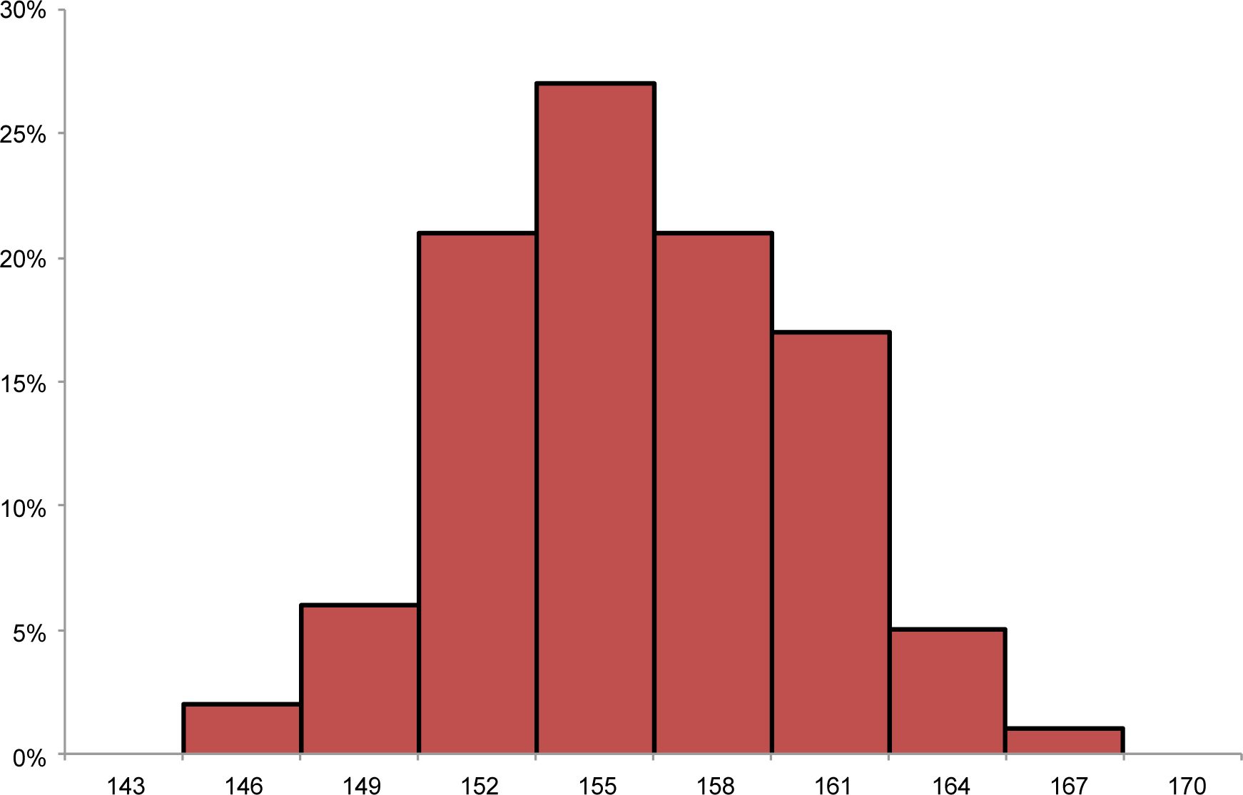
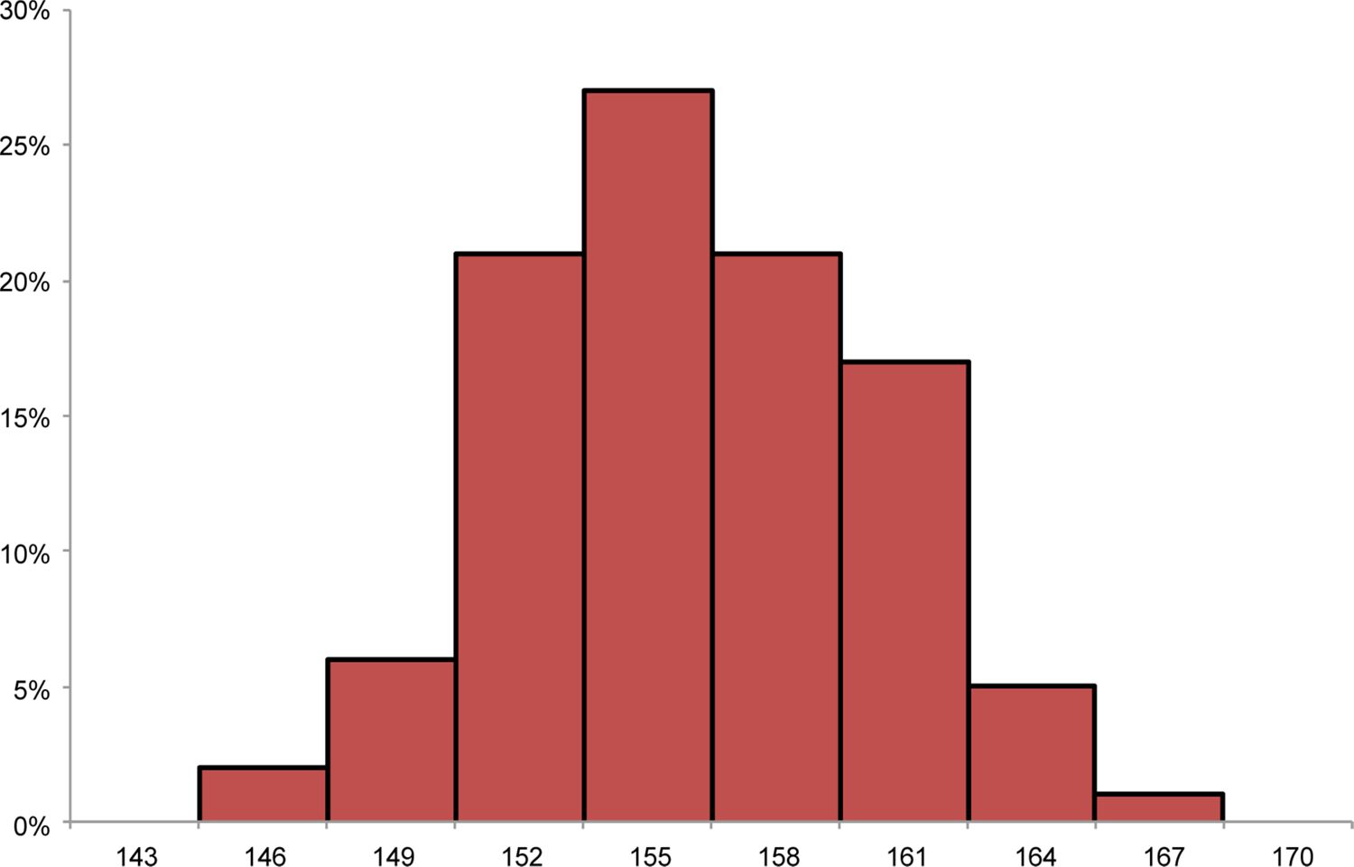
Recall that we report simulation results using data that are aggregated over 100 distinct simulation runs so as to ensure that average measures of the model’s outcomes across runs are not influenced unduly by outliers. Figure 8 reports the distribution of simulated pregnancy rates among unmarried women across 100 runs of the model, and Figure 9 reports the same for married women. For both groups, the pregnancy-rate distribution across runs is unimodal and roughly symmetric.

Distribution of annual non-marital pregnancy rates per 1,000 women, across simulation runs.
Source: Results were generated using data from 100 one-year steady-state runs of the FamilyScape 3.0 model.
Distribution of annual marital pregnancy rates per 1,000 women, across simulation runs.
Source: Results were generated using data from 100 one-year steady-state runs of the FamilyScape 3.0 model.
2.4 Stage IV: maternal and child outcomes
FamilyScape models a number of different maternal and child outcomes for each simulated birth. For instance, because we record the marital status of each woman in the simulation, we also automatically track the structures of the families – specifically, whether they are married-parent or single-parent – into which children are born. For each live birth, the model also assigns a poverty status to the newborn child as a function of the mother’s demographic characteristics. FamilyScape’s child poverty module is parameterized using data from the March 2009 Current Population Survey, which contains income information for calendar year 2008.
We model several additional maternal and child outcomes using 2008 NVSS data. Given that being born at low birth weight is predictive of later health problems such as asthma, diabetes, and heart disease (Johnson & Schoeni, 2011), we model the probability that a newborn child will weigh less than 2,500 grams at birth. Evidence also suggests that children are more likely to experience a variety of negative outcomes if their mothers smoke or experience hypertension or diabetes during pregnancy (Gilland, Li, & Peters., 2001; Kim, Vohr, & Oh, 1996: Yessoufou & Moutairou, 2011). We therefore simulate maternal smoking, maternal hypertension, and maternal diabetes for pregnancies that will ultimately result in births. We use the results of NVSS-based regressions to vary women’s probabilities of experiencing these outcomes as a function of their demographic attributes.
Table 8 compares simulated and real-world estimates for each of these outcomes except family structure, which is benchmarked in Table 7. For all outcomes, FamilyScape produces simulated results that are similar to their real-world benchmarks.
Simulated and real-world maternal and child birth outcomes, by marital status.
| Unmarried Women | Married Women | |
|---|---|---|
| Simulated Data | ||
| Child Poverty | 50.8% (50.4%–51.2%) | 10.2% (10.0%–10.4%) |
| Low Birth Weight | 9.3% (9.1%–9.5%) | 7.0% (6.8%–7.2%) |
| Maternal Smoking | 19.6% (19.3%–19.9%) | 6.1% (5.9%–6.3%) |
| Maternal Diabetes | 3.8% (3.6%–4.0%) | 5.3% (5.1%–5.5%) |
| Maternal Hypertension | 4.3% (4.1%–4.5%) | 4.1% (4.0%–4.2%) |
| Real-World Data | ||
| Child Poverty | 54.5% | 9.9% |
| Low Birth Weight | 9.7% | 7.0% |
| Maternal Smoking | 16.3% | 5.5% |
| Maternal Diabetes | 3.6% | 5.0% |
| Maternal Hypertension | 4.0% | 3.9% |
-
Sources: Simulated results were generated using data from 100 one-year steady-state runs of the FamilyScape 3.0 model. Real-world benchmarks for child poverty were produced via analysis of the March 2009 Current Population Survey. Real-world benchmarks for all other outcomes were produced via analysis of 2008 data from the National Vital Statistics System.
-
Notes: Ninety-five percent confidence intervals are reported in parentheses beneath each simulated estimate. Confidence intervals reflect uncertainty related to random variation in simulation results across runs.
3. Parameter estimation
As previously discussed, we assign most of FamilyScape’s behavioural parameters to members of the simulation population using the results of regression analyses that were estimated using real-world data. Each of these regression models includes as covariates some or all of the demographic characteristics enumerated in Table 1. Many regressions also include controls for certain behavioural attributes. For example, when we estimate regressions models for the purpose of assigning an initial contraceptive type to each member of the simulation population, we control for annual sexual activity type and within-month coital frequency type. Likewise, we model the probability of contraceptive switching as a function of whether the woman was pregnant in the previous month and of her initial contraceptive type (i.e., the contraceptive type assigned to her at the outset of the simulation). For a woman who switches methods multiple times, we additionally condition the probability of “higher-order” switching on her most recent contraceptive type and on the number of times that she has switched methods during the current year.
Table 9 provides a summary of the covariates included in each set of regression equations. In addition, the table reports the number of unique outcomes that are modelled by each set of regressions and the number of equations required to model those outcomes. For instance, there are three possible outcomes for a given pregnancy (i.e., each pregnancy will result in a birth, an abortion, or a fatal loss), and we use two equations to model these three outcomes. One regression models the probability that a given pregnancy will result in an abortion; a second regression models the probability that the pregnancy will result in a birth given that it did not result in an abortion; and the residual probability reflects the likelihood that the pregnancy will result in a fatal loss. As is indicated in the table, we estimate separate regression equations for married and unmarried women for each outcome.29 The table also describes the functional form for each set of regressions. As an example, we use the results of hazard models to simulate contraceptive method switching (this approach allows the probability of switching to vary as a function of analysis time), and we use the results of logistic regression models to simulate the choice of contraception among women who switch methods.30 In Appendix A, we report results for all of the regressions used to estimate FamilyScape’s parameters.
Overview of FamilyScape’s regression specifications.
| Regression Characteristics | Dependent Variable | ||||
|---|---|---|---|---|---|
| Annual Sexual Activity Type | Within-Month Coital Frequency Type | Initial Contraceptive Type | Probability of Switching Contraceptive Types For the first contraceptive switch a | Probability of Switching Contraceptive Types For higher-order contraceptive switchesb | |
| Separate Equations Estimated by Marital Status? | Y | Y | Y | Y | Y |
| Number of Outcomes | 3 | 3 | 8 | 2 | 2 |
| Number of Regressions Estimated for Each Marital-Status Category | 2 | 2 | 7 | 7 (for unmarried women) 6 (for married women) | 1 |
| Functional Form | Logistic Regression | Logistic Regression | Logistic Regression | Logistic Hazard | Logistic Hazard |
| Demographic Covariates: | |||||
| Age | ✓ | ✓ | ✓ | ✓ | ✓ |
| Race | ✓ | ✓ | ✓ | ✓ | ✓ |
| Education | ✓ | ✓ | ✓ | ✓ | ✓ |
| Socioeconomic Status | ✓ | ✓ | ✓ | ✓ | ✓ |
| Behavioral Covariates: | |||||
| Annual Sexual Activity Type | ✓ | ✓ | |||
| Within-Month Coital Frequeny Type | ✓ | ||||
| Pregnant in the Previous Month | ✓ | ✓ | |||
| Number of Previous Contraceptive Switches | ✓ | ||||
| Origin Contraceptive Type | ✓ | ✓ | |||
| Most Recent Contraceptive Type | ✓ | ||||
| Regression Characteristics | Dependent Variable | ||||
| New Contraceptive Type After the first method switch 3 | New Contraceptive Type After higher-order method switches 3 | Pregnancy Outcomes Among women who experience a pregnancy | Probability that a Child will be Born into Poverty Among women whose pregnancy results in a birth | ||
| Separate Equations Estimated by Marital Status? | Y | Y | Y | Y | |
| Number of Outcomes | 8 | 8 | 3 | 2 | |
| Number of Regressions Estimated for Each Marital-Status Category | 7 | 7 | 2 | 1 | |
| Functional Form | Logistic Regression | Logistic Regression | Ordinary Least Squares | Linear Probability Model | |
| Demographic Covariates: | |||||
| Age | ✓ | ✓ | ✓ | ✓ | |
| Race | ✓ | ✓ | ✓ | ✓ | |
| Education | ✓ | ✓ | ✓ | ||
| Socioeconomic Status | ✓ | ✓ | |||
| Behavioral Covariates: | |||||
| Annual Sexual Activity Type | |||||
| Within-Month Coital Frequency Type | |||||
| Pregnant in the Previous Month | ✓ | ✓ | |||
| Number of Previous Contraceptive Switches | ✓ | ||||
| Origin Contraceptive Type | ✓ | ✓ | |||
| Most Recent Contraceptive Type | ✓ | ||||
| Regression Characteristics | Dependent Variable | ||||
| Probability that a Child will be Born at Low Birth Weight Among women whose pregnancy results in a birth | Probability of Maternal Smoking Among women whose pregnancy results in a birth | Probability of Maternal Diabetes Among women whose pregnancy results in a birth | Probability of Maternal Hypertension Among women whose pregnancy results in a birth | ||
| Separate Equations Estimated by Marital Status? | Y | Y | Y | Y | |
| Number of Outcomes | 2 | 2 | 2 | 2 | |
| Number of Regressions Estimated for Each Marital-Status Category | 1 | 1 | 1 | 1 | |
| Functional Form | Logistic Regression | Logistic Regression | Logistic Regression | Logistic Regression | |
| Demographic Covariates: | |||||
| Age | ✓ | ✓ | ✓ | ✓ | |
| Race | ✓ | ✓ | ✓ | ✓ | |
| Education | ✓ | ✓ | ✓ | ✓ | |
| Socioeconomic Status | |||||
| Behavioral Covariates: | |||||
| Annual Sexual Activity Type | |||||
| Within-Month Coital Frequency Type | |||||
| Pregnant in the Previous Month | |||||
| Number of Previous Contraceptive Switches | |||||
| Origin Contraceptive Type | |||||
| Most Recent Contraceptive Type | |||||
-
Notes: All regression models described in this portion of the table were estimated using data on female NSFG respondents.
-
a
For the probability of switching methods for the first time, we estimate separate regressions for each origin contraceptive type except female sterilization (under the simplifying assumption that sterilized women will not undergo surgical reversal of their sterilization) and, for married women, male sterilization (under the simplifying assumptions that each woman who is married to a sterilized man will have the same spouse throughout the simulation and that her spouse will not undergo surgical reversal of his sterilization). All regressions also include a set of monthly baseline hazard dummy variables.
-
b
For higher-order switching, we do not estimate separate equations for each origin contraceptive method because of limited sample sizes. Rather, we estimate one model per marital-status group and include a series of "origin contraceptive type" dummies as covariates. All regressions also include a set of monthly baseline hazard dummy variables.
-
All regression models described in this portion of the table were estimated using data on female NSFG respondents except for: a) the pregnancy-outcome regressions, which additionally use data from the Nationalvital Statistics System and the Guttmacher Institute's Abortion Provider Survey; and b) the child-poverty regressions, which were estimated using Current Population Survey data.
-
c
These regression equations also include a continuous month variable and a quadratic month variable.
Overview of FamilyScape’s non-regression-estimated parameters.
| Dependent Variable | |||
|---|---|---|---|
| Female Fecunditya | Contraceptive Failureb | Gestation Periodsc | |
| Estimation Approach | Equations developed via syntheses of published studies | Original data tabulations | Synthesis of published estimates |
| Covariates | Age, day in menstrual cycle | Marital status, age, contraceptive type | Pregnancy outcome |
-
a
See the main text for a complete listing of the studies whose findings were used to generate FamilyScape's fecundity parameters.
-
b
FamilyScape's contraceptive failure probabilities are generated by plugging parameters that were estimated via analysis of data on female NSFG respondents (e.g., the monthly pregnancy rates and average within-month coital frequencies of women who use a given method, are of a given marital status, and fall into a given age category) into an equation that was developed for the purpose of modelling single-act contraceptive failure rates.
-
c
FamilyScape's gestation periods are extended to account for the period of time after a pregnancy ends during which a woman is infertile. The durations of these post-pregnancy infertility periods, like the gestation periods that precede them, vary according to the pregnancy's outcome. See the main text for a complete listing of the studies whose results were synthesized to generate the model's gestation-period and post-pregnancy-infertility parameters.
A smaller number of FamilyScape’s parameters were generated using an approach other than regression-based estimation. For instance, a fecundity level is imputed to each member of the simulation population on each day by plugging her age and the day in her menstrual cycle into one of several equations that we developed by synthesizing the results of a number of different clinical studies that were previously referenced.31 Similarly, a woman is assigned a contraceptive failure rate as a function of the method(s, if any) that she is using, her age, and her marital status. More specifically, we estimate subgroup failure rates by plugging the characteristics of each contraception-age-marital-status group (e.g., that group’s monthly pregnancy rate and average monthly coital frequency) into Equation 3, which was developed specifically for the purpose of modelling single-act contraceptive failure rates within FamilyScape’s simulation framework.32 Table 10 briefly describes the estimation approach that was used to develop each of FamilyScape’s nonregression-based parameters. The table also reports the demographic and/or behavioural dimensions along which these parameters vary. As an example, a pregnancy’s gestation period varies only according to the pregnancy’s outcome (e.g., a birth will have a notably longer gestation period than will an abortion or a fatal loss).33
4. Discussion
FamilyScape 3.0 successfully reproduces real-world variation in the most important proximate antecedents of pregnancy, including sexual activity, contraceptive behaviour, and female fecundity. Perhaps most importantly, the model generates aggregate rates of contraceptive failure, pregnancy, birth, abortion, and maternal and child outcomes that closely match their real-world equivalents. Data from numerous sources are integrated into the model’s simulation structure in order to ensure that these behaviours and outcomes vary realistically according to marital status, age, race, educational attainment, and SES.
FamilyScape also has important limitations. Our results suggest that the model is better suited to analyses that focus on broadly defined groups (for example, unmarried women) than to analyses that focus on more narrowly defined groups (for example, young unmarried nonwhite women). Also important is the fact that FamilyScape only accounts for a limited number of individual attributes. However, given the precision with which the model replicates real-world fertility outcomes at the aggregate level for both married and unmarried women, we believe that it holds considerable promise as a policy analysis tool.
We intend to use FamilyScape to project the impacts of a variety of different policy interventions. To the extent that external estimates are available regarding policies’ effects on sexual and contraceptive behaviours, the model can be used to project the implications of these behavioural impacts for rates of pregnancy, childbearing, abortion, child poverty, low birth weight, and so forth. For example, in the wake of the ACA’s implementation, researchers will undoubtedly estimate its impacts on contraceptive behaviour. FamilyScape can then be used to study the implications of these behavioural changes for a range of different outcomes. As another example, several recent studies have shown that rates of unintended pregnancy can be dramatically reduced by increasing access to LARC methods (Harper et al., 2015; Ricketts, Klingler, & Schwalberg, 2014; Winner et al., 2012). This body of evidence has led some researchers to conclude that future reductions in unintended pregnancy may require expanded use of LARC methods (Peipert, Madden, Allsworth, & Secura; Secura, 2013). We plan to use FamilyScape to test this hypothesis by assessing the extent to which pregnancy rates could be reduced via increases in the use of other forms of contraception, such as condoms and PPR methods. More broadly, our expectation is that FamilyScape will be used to answer a host of important policy questions, especially given that considerations of family structure feature so prominently in contemporary social policy debates in the United States.
Footnotes
1.
Several simulation models of fertility were created in the 1960s and 1970s (Barrett, 1971; Guthrie, Orcutt, Caldwell, Peabody, & Sandowsky, 1975; Ridley & Sheps, 1966). More recently, researchers have developed models of European fertility (Carioli & Devolder, 2016; Thomson, Winkler-Dworak, Spielauer, & Prskawetz, 2012). Other recent US-focused simulation models also contain fertility modules (Favreault, Smith, & Johnson, 2015; Holmer, Janney, & Cohen, 2006; Smith & Favreault, 2013), although fertility is not the primary focus of any of these models. As a consequence, none of these models explicitly simulates the most important behavioural and biological determinants of pregnancy such as sexual activity, fecundity, contraceptive use, and contraceptive efficacy. Thus, there is a dearth of models that focus specifically on fertility in the United States, and that explicitly simulate the key antecedents of pregnancy and childbearing.
2.
More specifically, the policy’s impacts can be estimated by comparing results produced by the model’s baseline specification with results produced by the relevant policy specification (see Appendix B for additional discussion of this topic). Critical to the plausibility of such a simulation is the existence of credible external evidence regarding the policy’s effects on the behaviours that FamilyScape simulates. To the extent that there is uncertainty about the magnitudes of such behavioural effects, sensitivity analysis can and should be performed in order to produce a range of simulated estimates. See Thomas (2012b) for an example of such an approach. We would also note that FamilyScape does not model the socioemotional traits (e.g., self-control and risk preferences) that govern these behaviours. In other words, the model can easily be used to simulate changes in individual behaviours, but it does not allow for explicitly simulated changes in the underlying socioemotional attributes that animate those behaviours.
3.
For other examples of single-sex simulation models of fertility and family formation, see Lutz (1997) and Sajjad and Ahn (2014).
4.
Appendix C provides pseudocode for each of FamilyScape’s modules.
5.
Static models such as FamilyScape are distinguished by the fact that they do not allow individuals within the simulation to age or evolve as analysis time passes. In most respects, then, FamilyScape functions as a steady-state model that reproduces in perpetuity the general conditions that were observed in the real-world data used to develop its baseline parameters. As an example, the model continuously replicates real-world coital frequency distributions and pregnancy-outcome distributions from 2006 – 2010. The lone exception to this rule is FamilyScape’s contraceptive switching module, which is a dynamic component of the model that systematically changes the contraceptive mix among the members of the simulation population over time. This dimension of the model is described in the discussion of “Stage II” in the main text. For more information on microsimulation models in general and on static models in particular, see Citro and Hanushek (1991), Harding (2007), Merz (1994), and Mitton, Sutherland, and Weeks (2000).
6.
Numerous academic studies and government reports find that there is substantial variation in contraceptive behaviours and fertility outcomes according to these characteristics. As just a few examples, Daniels, Daugherty, and Jones (2014) find that female sterilization is three times as likely to be used by women without a high-school degree as by women with a college diploma, while women in the latter category are nearly six times as likely as women in the former category to use oral contraception; Finer and Zolna (2016) find that the rate of unintended pregnancy is more than five times as high among economically disadvantaged women as among women who are not economically disadvantaged and that pregnancies among unmarried women are more than twice as likely as pregnancies among married women to result in abortion; Jones et al. (2012) find that contracepting women in their late twenties are more than four times as likely as contracepting women in their late thirties to rely on male sterilization and that non-Hispanic black women are almost twice as likely as non-Hispanic white women not to use contraception when they are at risk of unintended pregnancy; and Mosher et al. (2015) find that, among women at risk of unintended pregnancy, the probability of using contraception during intercourse is statistically significantly related to marital status, age, race, and educational attainment.
7.
The primary exception to this rule is the fact that FamilyScape’s simulated pregnancy rate for women over 40 is nontrivially higher than the corresponding real-world benchmark. This issue is discussed further in a subsequent section of the paper.
8.
More precisely, respondents are asked about their contraceptive histories during a period spanning from January of the calendar year three years prior to the interview date until the present. Thus, for example, a woman surveyed in February would provide 38 months of contraceptive calendar data, while a woman surveyed in December would provide a full 48 months’ worth of data (NCHS, 2011).
9.
In fact, the 2006 – 2010 NSFG contains only about 12,000 female respondents in total. We extract a simulation population of 20,000 women by sampling observations with replacement. We oversample NSFG respondents in order to increase the size of the simulation population, which in turn improves the precision of our simulated estimates. See Appendix B for further discussion of this issue.
10.
On the use of maternal education as a proxy for socioeconomic status, see Bornstein, Hahn, Suwalsky, and Haynes (2003).
11.
A partial exception to this rule is marital status, which is cited almost universally in the literature as an important correlate of sexual behaviour, contraceptive use, and fertility outcomes (Finer & Zolna, 2016; Gamble et al., 2008; Goldin and Katz, 2002; Jones et al., 2002, 2012; Martin et al., 2015; Martin, Hamilton, Osterman, Curtin, & Mathews, 2015; Mosher et al., 2015; Thomas & Monea, 2009; Ventura, Abma, Mosher, & Henshaw, 2008; Vespa et al., 2012). Importantly, however, we treat marital status as a fixed characteristic for the purposes of our simulations. As previously discussed, we do not simulate the formation of new marriages or the dissolution of existing ones. We also estimate all of FamilyScape’s parameters using real-world data on women whose marital status does not change during the period in which we observe them.
12.
The “high school degree” education category contains women who have earned either a high school diploma or a General Educational Development credential but have not pursued any further formal education. The “other” race category encompasses Asians, Native Americans, and all other women who do not self-identify as white non-Hispanic, black non-Hispanic, or Hispanic. In exploratory work conducted when the first version of FamilyScape was being developed, we considered the possibility of using several alternate specifications of education and age. For education, we also considered models using a continuous variable. For age, we considered models using a continuous variable; continuous and quadratic terms; and continuous, quadratic, and cubic terms. According to the results of numerous statistical tests, the variable specifications described in Table 1 usually performed at least as well as – if not better than – these alternate specifications. As previously discussed, we use maternal education as a proxy for SES. We considered several different specifications of SES in our regression analyses. Specifically, we considered a continuous variable, a four-category variable (less than high school, high-school degree, some college, and a college degree or more), and a tripartite variable (less than high school, high-school degree, and more than high school). The results of various statistical tests indicated that a dummied version of this variable was preferable, although it was not obvious whether the variable’s breakpoint should be at “less than a high-school degree/at least a high school degree” or at “high school degree or less/some college.” We chose to use the former breakpoint because this definition of SES has the advantage of producing a slightly more balanced distribution.
13.
In most of our tables, we report confidence intervals for our simulated estimates. These confidence intervals reflect uncertainty related to random variation in our results across simulation runs. We do not report confidence intervals for Table 2 because we use the same simulation population for all runs (thus, there is no variation in the composition of the simulation population across runs).
14.
Given that we are interested in modelling the incidences of pregnancy and childbearing, FamilyScape’s sexual behaviour modules only simulate the occurrence of heterosexual vaginal intercourse.
15.
This conclusion is based on our analysis of data taken from the NSFG’s “periods of non-intercourse” module, in which women are asked whether they were sexually active in each of the twelve months leading up to the interview month (e.g., “Did you have sex last October?”; “Did you have sex last September?”; and so forth).
16.
This conclusion is based on our analysis of responses to the following NSFG survey question: “Now please think about the last four weeks. How many times have you had sexual intercourse with a male in the last four weeks?” Once a woman is placed in a within-month coital frequency category, we scale up her initially imputed four-week coital frequency by 1.07 (30/28) in order to assign her a full-month coital frequency level.
17.
18.
We use the term “sterilization” to refer both to natural sterility and to surgical sterilization. The following contraceptive methods are considered to be LARC methods for the purposes of this discussion: intrauterine devices, hormonal implants, and injectables. The PPR category captures women who use oral contraception, the contraceptive patch, the NuvaRing, and emergency contraception. For purposes of simplicity, we also assign the small proportion of women in the NSFG who use other non-hormonal, female-controlled contraceptive methods to the PPR category. These methods include diaphragms, female condoms, foams, jellies/creams, suppositories/inserts, the contraceptive sponge, and natural family planning.
19.
Because withdrawal is a male-controlled method, and for purposes of simplicity, we collapse condom users and users of withdrawal into a single contraceptive category. Thus, a woman whose partner uses withdrawal is considered to rely on condoms for the purposes of FamilyScape’s simulations. Condoms and withdrawal have roughly similar levels of efficacy (Trussell, 2011).
20.
There are two exceptions to this general rule. Specifically, we do not model contraceptive switching among sterilized women or among married women whose partners are sterilized. These exceptions are rooted in the fact that, during a given year, sterilized women rarely undergo surgical reversal of their sterilization and married women rarely discontinue the use of male sterilization (Thomas & Karpilow, 2015).
21.
There are a limited number of instances in which simulated and real-world switching estimates diverge noticeably. Specifically, the across-month distribution of simulated method choice for married women in the “LARC & Condom” origin category differs nontrivially from the equivalent real-world distribution. As is shown in Table 3, however, only three tenths of one percent of married women fall into this contraceptive category. These differences between simulated and real-world switching behaviours are thus a function of the very limited amount of data that are available to model switching behaviour among women in this category. This type of imprecision has virtually no impact on FamilyScape’s aggregate simulation results because it is relevant for only a handful of women. Indeed, while developing the current version of FamilyScape, we experimented with a number of different parametric approaches to simulating method switching among members of small contraceptive groups. The model’s simulated pregnancy, birth, and abortion rates were essentially unchanged across these various specifications. For all contraceptive categories other than the one referenced here, simulated and real-world switching behaviours are much better aligned. Taken as a whole, then, the results reported in Tables 4 and 5 indicate that FamilyScape produces realistic patterns of method switching for contraceptive categories that contain more than a very small number of women.
22.
The mean age of the participants in the Royston’s sample was 32, and he estimates the values of χ0 and X1 to be .48 and .022, respectively. The latter two parameters are used to measure the (age-specific) probability that a woman is capable of becoming pregnant in a given cycle. This probability is less than one for a variety of reasons. For instance, in any given menstrual cycle, it is possible that: a) ovulation does not occur; b) defects in the egg preclude any possibility of fertilization; or c) the embryo aborts prior to being registered as a pregnancy in the author’s study. Thus, the bracketed portion of Equation 1 reflects the probability that such events do not occur. The “αt” component of Equation 1 is modeled using the following functional form: αt = exp(-[tov − t]/λs) for all t < tov, αt = 1 for t =tov; and αt = exp(-[t − tov]/λe> for all t > tov, where t is an index for the day in the menstrual cycle, tov is the day of ovulation, λe is the average life of the egg in days, and λs is the average life of the sperm in days. Royston estimates the value of λs to be 1.47, and he estimates the value of λe to be .7.
23.
We also make series of additional adjustments to Royston’s fecundity estimates. Our fecundity adjustments are described in detail in Thomas and Karpilow (2015).
24.
Our contraceptive efficacy estimates are calculated under the assumption that the user does not switch methods or discontinue contraceptive use. Thus, the dimension of “consistency” that is captured by our efficacy estimates corresponds not to the propensity to switch methods but instead to the likelihood of (for example) missing a certain number of pills per month. We would also note that we model a “failure rate” for noncontraceptors. In other words, even for a woman not using any contraception, we use the approach described above to adjust downward the predicted probability of pregnancy from a single act of intercourse that is initially assigned to her as a function of our fecundity equations. We make this adjustment based in large part on evidence demonstrating that, in point of fact, women who self-report as noncontraceptors often rely on withdrawal and/or natural family planning methods (Jones, Lindberg, & Higgings, 2014; Jones, Fennell, Higgins, & Blanchard, 2009; Potts & Diggory, 1983; Sinai, Lundgren, Arévalo, & Jennings, 2006). See Thomas and Karpilow (2015) for further discussion of this topic.
25.
Jones et al. (2002) use data from a survey of abortion patients to estimate the distribution of the most effective form of contraception used during the month of conception among women obtaining abortions. We apply this distribution to Jones and Jerman’s (2014) tally of the total number of abortions in 2008 in order to approximate the number of abortions occurring to users of different methods. Because Jones and Jerman’s abortion count is based on a survey of all known abortion providers, we assume that their estimate reflects the true number of abortions in the United States in 2008. Next, we use the NSFG to tabulate the annual number of self-reported abortions, disaggregated by the most effective method used during the conception month. For each contraceptive category j (including the category corresponding to the use of no method), we then compute the following:
where gj is the pregnancy inflation factor for users of method j; is the (uncorrected) number of pregnancies occurring to users of method j as estimated using NSFG data; is the (uncorrected) number of abortions occurring to users of method j as estimated using the NSFG; and is the “true” number of abortions occurring to users of method j as measured using data reported in Jones et al. (2002) and Jones and Jerman (2014). Note, then, that our estimates of gj are method-specific ratios of the abortion-undercount-corrected number of annual pregnancies to the uncorrected, NSFG-based count of pregnancies. We apply these ratios (gj) to our NSFG-derived monthly pregnancy rates in order to produce estimates of abortion-undercount-corrected, method-specific monthly pregnancy rates. Given that Jones et al. (2002) do not produce demographically disaggregated estimates of method-specific abortion counts, we are compelled to assume that the extent of abortion underreporting in the NSFG does not vary systematically between demographic groups within a given contraceptive category. And because Jones and her co-authors analyse data on contraceptive use among abortion patients in 2000 – 2001, we also implicitly assume that the distribution of abortions by method use did not change between this period and the 2006 – 2010 time frame to which FamilyScape is calibrated. We would prefer to have used more recent data and to have allowed our undercount estimates to vary demographically, but the Jones et al. (2002) paper is the most recent study to report estimates of the distribution of abortions by contraceptive method.
26.
More precisely, we use the above-referenced data sources to generate tabulations of the total number of births, abortions, and foetal losses that occurred in 2008. Given the limitations of the available real-world data, we are able to disaggregate these tabulations only according to age and race. We use these data to estimate, for each age-race subgroup, the share of pregnancies that result in each of these three outcomes. Next, we use these estimates to assign a set of demographically specific pregnancy-outcome probabilities (reflecting the chances that a pregnancy will result in a birth, an abortion, or a foetal loss) to each member of FamilyScape’s simulation population. We then regress these probabilities on the age and race characteristics of the members of the simulation population. The results of these regressions are used to parameterize FamilyScape’s pregnancy-outcomes module. This approach allows us to incorporate substantially fewer parameters into the pregnancy-outcomes module than would have been the case if we had imported our original matrix of pregnancy-outcome probabilities directly into FamilyScape. Because these regressions control for the same set of characteristics as were used to develop our demographically specific pregnancy-outcome probabilities, their predictive power is very high (see Table A.12 in Appendix A).
27.
Information on gestation periods for live births was taken from Martin et al. (2013). For additional information on gestation periods for induced abortions, see Finer and Henshaw (2003), Gamble et al. (2008), Jones et al. (2008), and Jones and Kost (2007). For additional information on gestation periods for foetal losses, see Brown (2008), Everett (1997), MacDorman, Munson, and Kimeyer (2007), Nybo Anderson, Wohlfart, Christens, Olsen, and Melbye (2000), Ventura et al. (2008), and Wilcox, Weinberg, and Baird (1988). For additional information on postpartum infertility, see National Center for Chronic Disease Prevention and Health Promotion (2014), Hatcher et al. (2004), and Pinto and Palloni (1996); for additional information on post-abortion infertility, see Curtis, Huber, and Moss-Knight (2010) and World Health Organization (2007); and, for additional information on infertility after a foetal loss, see MD Health (2017) and MedicineNet (2016).
28.
Among the members of FamilyScape’s simulation population aged 15 – 39, women between the ages of 30 and 39 constitute a smaller share (23%) of the unmarried population than do women in any other age group, while teenagers constitute the smallest share (1%) of married women. Conversely, the groups for which FamilyScape performs especially well tend to be comparatively large. For example, women in their twenties represent the largest age group (45%) within the unmarried population, and women in their thirties comprise the largest share (65%) of the married population. As is discussed above, the model produces realistic results for unmarried women in their twenties. The same is generally true for married women in their thirties.
29.
A bit more of an explanation may be helpful to the reader regarding the number of outcomes and the number of regression equations used to implement the model’s contraceptive behaviour modules. As is discussed earlier in this paper, FamilyScape allows women to assume one of eight different contraceptive types, each of which corresponds to a different combination of female-controlled and male-controlled methods (or to the use of no female-controlled and/or no male-controlled contraception). More specifically, each woman is assigned to one of the following eight contraceptive categories: (1) no female-controlled method & no male-controlled method; (2) no female-controlled method & condom; (3) PPR & no male-controlled method; (4) PPR & condom; (5) LARC & no male-controlled method; (6) LARC & condom; (7) female not sterilized & male sterilized; and (8) female sterilized. Regarding these latter two categories, we do not model the choice of male-controlled methods for women who are sterilized or of female-controlled methods for women whose partners are sterilized because we make the simplifying assumption that sterilization is 100% effective (in other words, we assume that the use of methods other than sterilization will have no effect on the risk of becoming pregnant among women in the latter two contraceptive categories). With respect to the regressions that model initial contraceptive type and the choice of methods after a switch, we only need to estimate seven different equations, for the reasons outlined above. However, we take a different approach when modelling the probability of switching methods. More specifically, we estimate separate equations for every one of our “origin contraceptive types” with the exception of female sterilization (we make the simplifying assumption that sterilized women will not seek surgical reversal of their sterilization) and, for married women, male sterilization (we also make a simplifying assumption that married women with sterilized spouses will not change sexual partners during the simulation and that these women’s sterilized partners will not seek reversal of their sterilization). We define a woman’s “origin contraceptive type” as her contraceptive type at the beginning of the segment of analysis time over which we model the probability that she will switch methods. For each of these “method-specific” regressions, there are two outcomes: “switch” and “no switch.” Also relevant is the fact that, because of the limited amount of data in the NSFG on contraceptive switches that occur after a woman’s first switch, we are unable to estimate separate equations modelling the probability of “higher-order switching” for each origin contraceptive type. Instead, we estimate only one regression per marital-status group, and we include a series of contraceptive type fixed effects dummies as covariates in these regressions.
30.
As is noted at the bottom of Table 9, we include a set of month dummies to allow the baseline hazard to vary over time when we model the probability of switching methods. Although the equations that model the choice of methods after a contraceptive switch are not hazard models, we concluded after a set of exploratory analyses that these regressions should nonetheless include controls for the point in time at which the switch occurred. These time-period controls capture unobservable characteristics that are associated with both method selection and the length of time over which a female method switcher chose to remain on her origin method. In other words, these covariates help to account for the possibility that, among women who switch contraceptive methods, the preferences of those who wait relatively longer to do so may differ in systematic (but unmeasurable) ways from the preferences of those who switch relatively quickly. Due to sample-size limitations, however, we are unable to include a complete set of month dummies in our method-selection regressions. As such, we instead include in these regressions a continuous month variable and a quadratic month term.
31.
The pseudocode for the Assign Fecundity program in Appendix C contains all of the equations used to impute fecundity levels as a function of age and day in the menstrual cycle.
32.
The pseudocode for the Assign Contraceptive Failure Rate program in Appendix C provides a complete listing of FamilyScape’s single-act contraceptive failure rates.
33.
The pseudocode for the Assign Post Pregnancy Infertility Period program in Appendix C provides the lengths of FamilyScape’s combined gestation periods and post-pregnancy infertility intervals for each pregnancy outcome.
A. Parameter-estimation regressions
The tables below report results for each of the regressions used to estimate FamilyScape’s parameters pertaining to annual sexual activity, within-month coital frequency, initial contraceptive assignment, contraceptive switching, pregnancy outcomes, and birth outcomes.1 We would note that, due to small sample sizes and/or limited variation in our data, we are occasionally unable to estimate models that contain a full set of covariates. For instance, only eleven married women in our NSFG data are initially assigned to the “LARC & Condom” contraceptive category. As a result, we are unable to include all of our demographic controls in the initial contraceptive assignment regression that models married women’s probability of falling into this category. We therefore control only for age in this regression specification (see Table A.4). In all such cases, our goal was to extract as much information as possible from our data while still allowing for reliable estimation of our regression models.2
Logistic regression results for annual sexual activity, by marital status.
| Inactive | Highly Active | |||
|---|---|---|---|---|
| Unmarried Women | Married Women | Unmarried Women | Married Women | |
| Age:25–29 | −1.021***(.125) | 0.470(.655) | 0.549***(.111) | −0.344(.210) |
| Age:30–44 | −0.447***(.093) | 1.003*(.553) | 0.546***(.100) | −0.055(.190) |
| Education:High School Degree | −0.978***(.101) | −1.334***(.484) | 0.013(.113) | 0.577***(.208) |
| Education:More than High School | −0.752***(.088) | −0.379(.398) | −0.026(.108) | 0.353*(.190) |
| Race:Black | −0.434***(.092) | 0.054(.484) | −0.165*(.099) | −0.140(.180) |
| Race:Hispanic | −0.219**(.104) | −0.332(.471) | 0.021(.117) | 0.271(.186) |
| Race:Other | 0.332**(.164) | 0.498(.681) | 0.046(.207) | −0.385*(.225) |
| High SES | 0.309***(.105) | −0.637(.414) | −0.119(.110) | 0.256*(.151) |
| Pseudo R-Squared | .07 | .03 | .02 | .01 |
| N | 7,989 | 3,675 | 5,431 | 3,588 |
-
Sources: All regressions were estimated using data taken from the 2006 – 2010 National Survey of Family Growth.
-
Notes: Standard errors are reported in parentheses beneath each parameter estimate. One asterisk (*) indicates that the estimate is statistically significant at or beyond the .1 level, two asterisks (**) indicate that the estimate is significant at or beyond the .05 level, and three asterisks (***) indicate that the estimate is significant at or beyond the .01 level.
Logistic regression results for within-month coital frequency, by marital status.
| Low | High | |||
|---|---|---|---|---|
| Unmarried Women | Married Women | Unmarried Women | Married Women | |
| Age:25–29 | 0.058(.129) | 0.415*(.215) | −0.127(.180) | −0.339(.273) |
| Age:30–44 | 0.031(.121) | 0.828***(.197) | −0.280(.184) | −0.277(.247) |
| Education:High School Degree | 0.130(.135) | −0.230(.182) | −0.124(.201) | 0.077(.288) |
| Education:More than High School | −0.109(.123) | −0.353**(.171) | −0.474***(.183) | −0.021(.277) |
| Race:Black | 0.564***(.116) | −0.265(.163) | −0.080(.183) | 0.248(.255) |
| Race:Hispanic | −0.020(.138) | −0.172(.152) | −0.030(.189) | 0.251(.243) |
| Race:Other | −0.010(.241) | 0.311(.221) | −0.020(.385) | −0.441(.493) |
| High SES | −0.359***(.133) | 0.140(.143) | 0.195(.185) | −0.318(.235) |
| Annual Sexual Activity Fixed Effects? | Y | Y | Y | Y |
| Pseudo R-Squared | .05 | .03 | .02 | .02 |
| N | 3,920 | 3,235 | 1,997 | 1,830 |
-
Sources: All regressions were estimated using data taken from the 2006 – 2010 National Survey of Family Growth.
-
Notes: Standard errors are reported in parentheses beneath each parameter estimate. One asterisk (*) indicates that the estimate is statistically significant at or beyond the .1 level, two asterisks (**) indicate that the estimate is significant at or beyond the .05 level, and three asterisks (***) indicate that the estimate is significant at or beyond the .01 level. Each regression includes a set of annual sexual activity fixed effects dummies that measure the number of sexually active months over the course of the focal year.
Logistic regression results for initial contraceptive assignment, among unmarried women.
| No Method | Condom Only | PPR Only | PPR & Condom | LARC Only | LARC & Condom | Male Sterilization | |
|---|---|---|---|---|---|---|---|
| Age: 25–29 | −1.953***(.386) | −1.085***(.185) | −0.285*(.172) | −0.775***(.206) | 0.180(.201) | −0.473(.616) | 0.786(.707) |
| Age: 30–44 | −3.222***(.353) | −2.188***(.171) | −0.508***(.176) | −1.108***(.219) | −0.660***(.241) | −1.345**(.628) | 2.462***(.493) |
| Education: High School Degree | 0.082(.285) | 0.076(.187) | 0.626***(.209) | 0.563**(.242) | −0.077(.228) | −0.010(.406) | 1.360**(.583) |
| Education: More than High School | 0.584*(.314) | 0.954***(.181) | 1.089***(.192) | 1.084***(.205) | −0.606***(.212) | −0.504(.393) | 1.003*(.550) |
| Race: Black | 0.465(.283) | −0.280(.173) | −1.349***(.170) | −0.727***(.203) | 0.607***(.229) | 0.865**(.392) | −3.595***(.747) |
| Race: Hispanic | 0.635*(.337) | 0.059(.195) | −0.251(.189) | −0.541**(.264) | 0.718***(.229) | 0.245(.557) | −0.573(.622) |
| Race: Other | 0.811(.777) | −0.144(.363) | 0.006(.296) | −0.827**(.356) | −0.355(.396) | 0.205(1.137) | −1.221(1.028) |
| High SES | 0.164(.276) | 0.261(.170) | 0.274(.186) | 0.500*(.267) | −0.379*(.212) | 0.240(.438) | 0.405(.576) |
| Sexual Behavior Fixed Effects? | Y | Y | Y | Y | Y | Y | Y |
| Pseudo R-Squared | .23 | .21 | .13 | .10 | .07 | .06 | .20 |
| N | 989 | 2,247 | 2,969 | 3,439 | 3,732 | 3,812 | 3,885 |
-
Sources: All regressions were estimated using data taken from the 2006 – 2010 National Survey of Family Growth.
-
Notes: Standard errors are reported in parentheses beneath each parameter estimate. One asterisk (*) indicates that the estimate is statistically significant at or beyond the .1 level, two asterisks (**) indicate that the estimate is significant at or beyond the .05 level, and three asterisks (***) indicate that the the .01 level. Each regression includes a set of sexual behaviour fixed effects dummies that reflect interactions between annual sexual activity type and within-month coital frequency type.
Logistic regression results for initial contraceptive assignment, among married women.
| No Method | Condom Only | PPR Only | PPR & Condom | LARC Only | LARC & Condom | Male Sterilization | |
|---|---|---|---|---|---|---|---|
| Age: 25–29 | −0.770*(.454) | −0.777***(.272) | −0.664***(.232) | 0.146(.422) | −0.140(.310) | −0.566(1.255) | 1.639***(.602) |
| Age: 30–44 | −2.038***(.426) | −1.444***(.245) | −1.334***(.215) | −0.136(.408) | −0.353(.284) | −0.789(1.196) | 3.326***(.550) |
| Education: High School Degree | 0.648**(.289) | 0.182(.246) | 0.059(.252) | 0.293(.607) | 0.046(.295) | -- | 1.039***(.383) |
| Education: More than High School | 1 251***(.259) | 0.887***(.226) | 1.170***(.223) | 1.176*(.522) | −0.086(.260) | -- | 0.862**(.365) |
| Race: Black | 0.035(.238) | −0.553**(.242) | −0.425*(.234) | −0.550(.454) | 0.578*(.298) | -- | −1.712***(.385) |
| Race: Hispanic | 0.112(.245) | 0.322*(.195) | −0.077(.184) | −0.086(.358) | 0.329(.232) | -- | −0.412(.266) |
| Race: Other | 0.788**(.400) | 0.870***(.294) | −1.348***(.296) | 0.044(.384) | 0.627*(.354) | -- | −0.772*(.434) |
| High SES | 0.105(.219) | 0.120(.192) | 0.166(.183) | −0.377(.295) | −0.122(.232) | -- | 0.236(.218) |
| Sexual Behavior Fixed Effects? | Y | Y | Y | Y | Y | Y | Y |
| Pseudo R-Squared | .11 | .07 | .09 | .03 | .02 | .01 | .10 |
| N | 1,189 | 1,833 | 2,483 | 2,612 | 2,858 | 2,869 | 3,205 |
-
Sources: All regressions were estimated using data taken from the 2006 – 2010 National Survey of Family Growth.
-
Notes: Standard errors are reported in parentheses beneath each parameter estimate. One asterisk (*) indicates that the estimate is statistically significant at or beyond the .1 level, two asterisks (**) indicate that the estimate is significant at or beyond the .05 level, and three asterisks (***) indicate that the estimate is significant at or beyond the .01 level. Each regression includes a set of sexual behaviour fixed effects dummies that reflect interactions between annual sexual activity type and within-month coital frequency type.
Logistic hazard regression results for the probability of a first method switch, among unmarried women.
| Origin Contraceptive Type | |||||||
|---|---|---|---|---|---|---|---|
| No Method | Condom Only | PPR Only | PPR & Condom | LARC Only | LARC & Condom | Male Sterilization | |
| Age: 25–29 | −0.274*(.146) | −0.282***(.106) | −0.253**(.117) | 0.144(.166) | −0.715***(.183) | −0.711(.471) | 1.336(.924) |
| Age: 30–44 | −0.803***(.155) | −0.299***(.104) | −0.529***(.136) | 0.063(.193) | −0.752***(.236) | 0.062(.456) | 1.263(.983) |
| Education: High School Degree | 0.227(.146) | −0.098(.105) | −0.428***(.161) | −0.504***(.191) | −0.618***(.213) | −0.680*(.394) | −2.601**(1.111) |
| Education: More than High School | 0.485***(.155) | 0.004(.097) | 0.364**(.148) | −0.958***(.171) | −0.468**(.202) | −0.630*(.339) | −1.014(.723) |
| Race: Black | −0.268*(.139) | −0.272***(.095) | 0.595***(.126) | 0.194(.160) | 0.049(.208) | −0.896***(.296) | 1.487*(.803) |
| Race: Hispanic | 0.132(.156) | −0.074(.104) | −0.104(.158) | 0.179(.228) | 0.511(.239) | −0.358(.427) | −0.033(1.007) |
| Race: Other | −0.388(.289) | −0.345*(.195) | −0.131(.234) | 0.405(.341) | 0.630*(.369) | 0.013(.674) | 0.295(1.116) |
| High SES | 0.177(.137) | −0.019(.100) | −0.148(.158) | 0.061(.206) | −0.039(.206) | 0.287(.340) | −0.831(.885) |
| Pregnant Last Month | 2.138***(.197) | 2.38***(.232) | 2.775***(.357) | 2.96***(.524) | 3.69***(.739) | -- | -- |
| Pseudo R-Squared | .08 | .03 | .03 | .04 | .06 | .09 | .09 |
| N | 13,625 | 34,117 | 24,711 | 12,347 | 7,406 | 1,959 | 2,185 |
-
Sources: All regressions were estimated using data taken from the 2006 – 2010 National Survey of Family Growth.
-
Notes: Standard errors are reported in parentheses beneath each parameter estimate. One asterisk (*) indicates that the estimate is statistically significant at or beyond the .1 level, two asterisks (**) indicate that the estimate is significant at or beyond the .05 level, and three asterisks (***) indicate that the estimate is significant at or beyond the .01 level.
Logistic hazard regression results for the probability of a first method switch, among married women.
| Origin Contraceptive Type | ||||||
|---|---|---|---|---|---|---|
| No Method | Condom Only | PPR Only | PPR & Condom | LARC Only | LARC & Condom | |
| Age: 25–29 | −0.341(.208) | −0.254(.205) | −0.009(.147) | −0.062(.300) | −0.559*(.316) | −0.346(1.006) |
| Age: 30–44 | −0.772***(.181) | −0.441**(.187) | −0.359***(.139) | −0.617**(.306) | −1.121***(.321) | −3.254***(.934) |
| Education: High School Degree | −0.249(.234) | 0.065(.244) | −0.146(.242) | −0.434(.643) | −0.682**(.308) | -- |
| Education: More than High School | 0.090(.217) | 0.347*(.211) | −0.216(.232) | −0.718(.665) | −0.299(.298) | -- |
| Race: Black | −0.364*(.204) | −0.403*(.241) | −0.006(.187) | −0.596(.534) | −0.364(.417) | -- |
| Race: Hispanic | −0.047(.197) | 0.386**(.183) | −0.270(.185) | −1.027(.660) | 0.164(.350) | -- |
| Race: Other | −0.564*(.305) | −0.951***(.242) | 0.278(.238) | −1.450***(.533) | 0.170(.421) | -- |
| High SES | −0.032(.178) | −0.018(.177) | 0.031(.169) | −.333(.521) | −0.226(.341) | -- |
| Pregnant Last Month | 3.180***(.200) | 3.348***(.390) | 3.167***(.432) | 2.621***(.720) | -- | -- |
| Pseudo R-Squared | .13 | .06 | .02 | .10 | .04 | .27 |
| N | 17,420 | 20,182 | 21,830 | 3,749 | 7,949 | 220 |
-
Sources: All regressions were estimated using data taken from the 2006 – 2010 National Survey of Family Growth.
-
Notes: Standard errors are reported in parentheses beneath each parameter estimate. One asterisk (*) indicates that the estimate is statistically significant at or beyond the .1 level, two asterisks (**) indicate that the estimate is significant at or beyond the .05 level, and three asterisks (***) indicate that the estimate is significant at or beyond the .01 level.
Logistic hazard regression results for the probability of a higher-order method switch, by marital status.
| Unmarried Women | Married Women | |
|---|---|---|
| Age: 25–29 | −0.049(.074) | −0.169(.141) |
| Age: 30–44 | 0.029(.086) | −0.194(.138) |
| Education: High School Degree | −0.084(.083) | 0.127(.210) |
| Education: More than High School | −0.171**(.079) | 0.187(.197) |
| Race: Black | −0.022(.072) | 0.040(.183) |
| Race: Hispanic | 0.049(.087) | 0.250(.154) |
| Race: Other | −0.370**(.161) | 0.028(.214) |
| High SES | 0.045(.079) | 0.045(.137) |
| Pregnant Last Month | 1.940***(.177) | 2.898***(.214) |
| Number of Previous Switches | 0.531***(.038) | 0.416***(.077) |
| Origin Contraceptive Type Fixed Effects? | Y | Y |
| Most Recent Contraceptive Type Fixed Effects? | Y | Y |
| Pseudo R-Squared | .08 | .12 |
| N | 21,405 | 9,559 |
-
Sources: All regressions were estimated using data taken from the 2006 – 2010 National Survey of Family Growth.
-
Notes: Standard errors are reported in parentheses beneath each parameter estimate. One asterisk (*) indicates that the estimate is statistically significant at or beyond the .1 level, two asterisks (**) indicate that the estimate is significant at or beyond the .05 level, and three asterisks (***) indicate that the estimate is significant at or beyond the .01 level. Each regression includes a set of fixed effects dummies that control for origin contraceptive type and most recent contraceptive type.
Logistic regression results for method selection after a first method switch, among unmarried women.
| Dependent Variable: New Contraceptive Type | |||||||
|---|---|---|---|---|---|---|---|
| Condom Only | PPR Only | PPR & Condom | LARC Only | LARC & Condom | Male Sterilization | Female Sterilization | |
| Age: 25–29 | −0.506**(.230) | −0.027(.165) | −0.537***(.174) | −0.020(.231) | −0.164(.350) | 1.182**(.520) | 1.516***(.383) |
| Age: 30–44 | −0.321(.270) | −0.231(.175) | −0.901***(.223) | −0.188(.267) | −0.401(.312) | 2.653***(.406) | 2.441***(.333) |
| Education: High School Degree | 0.303(.264) | −0.118(.179) | 0.191(.207) | −0.214(.227) | −0.117(.343) | 0.904(.552) | 0.140(.338) |
| Education: More than High School | 0.907***(.260) | 0.143(.169) | 0.968***(.188) | −0.189(.238) | −0.399(.323) | 0.255(.520) | −0.269(.351) |
| Race: Black | −0.259(.243) | −0.646***(.158) | −0.567***(.177) | 0.073(.200) | 0.846***(.273) | −2.218***(.494) | −0.698**(.300) |
| Race: Hispanic | −0.036(.253) | 0.101(.189) | −0.338*(.201) | 0.072(.254) | −0.147(.447) | −0.694*(.388) | −0.185(.365) |
| Race: Other | −0.321(.422) | 0.499*(.301) | −0.469(.353) | −0.073(.463) | 0.352(.505) | −0.562(.920) | .043(.556) |
| High SES | 0.508**(.254) | 0.381**(.180) | 0.340*(.207) | −0.331(.241) | 0.043(.326) | 0.884**(.412) | −0.462(.293) |
| Pregnant Last Month | −1.96***(.556) | 0.311(.303) | −0.485(.428) | 1.268***(,327) | −0.856(.597) | -- | 1 244***(.363) |
| Number of Months at Risk Of First Switch | −0.087(.144) | 0.074(.102) | −0.051(.106) | −0.015(.126) | −0.156(.176) | .0536(.268) | 0.019(.201) |
| Number of Months at Risk Of First Switch Squared | 0.006(.011) | −0.006(.008) | −0.004(.008) | −0.001(.001) | 0.009(.013) | −0.003(.019) | 0.000(.016) |
| Origin Contraceptive Type Fixed Effects? | Y | Y | Y | Y | Y | Y | Y |
| Pseudo R-Squared | .11 | .05 | .14 | .09 | .12 | .20 | .20 |
| N | 1,140 | 2,361 | 3,056 | 3,735 | 4,016 | 3,978 | 4,399 |
-
Sources: All regressions were estimated using data taken from the 2006 – 2010 National Survey of Family Growth.
-
Notes: Standard errors are reported in parentheses beneath each parameter estimate. One asterisk (*) indicates that the estimate is statistically significant at or beyond the .1 level, two asterisks (**) indicate that the estimate is significant at or beyond the .05 level, and three asterisks (***) indicate that the estimate is significant at or beyond the .01 level. Each regression includes a set of fixed effects dummies that that control for origin contraceptive type.
Logistic regression results for method selection after a first method switch, among married women.
| Dependent Variable: New Contraceptive Type | |||||||
|---|---|---|---|---|---|---|---|
| Condom Only | PPR Only | PPR & Condom | LARC Only | LARC & Condom | Male Sterilization | Female Sterilization | |
| Age: 25–29 | −0.878***(.299) | −0.243(.267) | −0.120(.339) | −0.316(.328) | −1.079(1.036) | 0.519(.891) | 0.489(.430) |
| Age: 30–44 | −0.341(.286) | −0.606**(.266) | −0.129(.327) | −0.040(.303) | −1.171(.953) | 2.229***(.851) | 1.539***(.359) |
| Education: High School Degree | 0.876*(.045) | 0.255(.367) | 1.249**(.612) | −1.184***(.365) | −0.443(1.145) | 0.493(.625) | −0.441(.418) |
| Education: More than High School | 0.669(.418) | 0.368(.341) | 1.225**(.554) | −0.958***(.309) | −0.552(1.241) | 0.217(.560) | −1.273***(.428) |
| Race: Black | −0.524(.467) | 0.388(.318) | −0.273(.474) | −0.099(.528) | 0.036(.947) | −0.876(.648) | 0.446(.403) |
| Race: Hispanic | 0.361(.335) | −0.120(.307) | −0.386(.382) | 0.435(.286) | −1.154*(.692) | −0.185(.396) | 0.763**(.384) |
| Race: Other | −0.318(.527) | −0.185(.347) | −0.920**(.439) | 0.144(.486) | −1.394(1.124) | −0.077(.604) | 0.663(.475) |
| High SES | −0.411(.298) | −0.256(.280) | −0.323(.326) | −0.017(.283) | 0.859(.657) | 0.462(.402) | 0.351(.370) |
| Pregnant Last Month | −0.130(.682) | −0.344(.326) | −0.578(.556) | 0.116(.352) | 2.603***(.877) | −2.954***(.851) | 0.754**(.361) |
| Number of Months at Risk Of First Switch | 0.029(.180) | −0.151(.147) | 0.015(.194) | −0.012(.188) | −0.513(.490) | 0.438*(.231) | −0.017(.192) |
| Number of Months at Risk Of First Switch Squared | −0.003(.014) | 0.009(.012) | −0.006(.015) | 0.001(.015) | 0.033(.036) | −0.034**(.017) | 0.008(.014) |
| Origin Contraceptive Type Fixed Effects? | Y | Y | Y | Y | Y | Y | Y |
| Pseudo R-Squared | .06 | .10 | .05 | .06 | .23 | .12 | .14 |
| N | 754 | 1,000 | 1,584 | 1,710 | 1,880 | 1,999 | 2,144 |
-
Sources: All regressions were estimated using data taken from the 2006 – 2010 National Survey of Family Growth.
-
Notes: Standard errors are reported in parentheses beneath each parameter estimate. One asterisk (*) indicates that the estimate is statistically significant at or beyond the .1 level, two asterisks (**) indicate that the estimate is significant at or beyond the .05 level, and three asterisks (***) indicate that the estimate is significant at or beyond the .01 level. Each regression includes a set of fixed effects dummies that that control for origin contraceptive type.
Logistic regression results for method selection after a higher-order method switch, among unmarried women.
| Dependent Variable: New Contraceptive Type | |||||||
|---|---|---|---|---|---|---|---|
| Condom Only | PPR Only | PPR & Condom | LARC Only | LARC & Condom | Male Sterilization | Female Sterilization | |
| Age: 25–29 | 0.128(.373) | 0.002(.198) | 0.250(.242) | 0.349(.269) | 0.158(.433) | 1.142*(.640) | 1.198**(.577) |
| Age: 30–44 | −0.024(.451) | 0.117(.256) | −0.336(.276) | −0.167(.293) | 0.008(.401) | 2.74**(.620) | 1.536**(.499) |
| Education: High School Degree | −0.962**(.338) | 0.163(.238) | −0.071(.277) | −0.289(.331) | 0.067(.505) | −0.155(.527) | −0.059(.482) |
| Education: More than High School | −0.032(.344) | 0.193(.234) | 0.965**(.239) | −0.916**(.279) | −0.370(.536) | −0.233(.505) | −0.685(.458) |
| Race: Black | −0.552*(.310) | −0.849**(.202) | −0.742**(.212) | −0.600(.244) | 0.732**(.315) | −2.101**(.850) | −0.213(.604) |
| Race: Hispanic | −0.450(.357) | −0.088(.242) | −0.093(.279) | 0.012(.300) | 0.542(.594) | −0.676(.703) | −0.051(.491) |
| High SES | 0.150(.329) | −0.061(.225) | 0.017(.257) | −0.026(.275) | 0.236(.448) | 0.674(.841) | 0.216(.483) |
| Pregnant Last Month | −1.338*(.789) | 1.436**(.300) | −0.732(.559) | 0.553(.349) | 0.713(.703) | −2.212**(1.115) | 1.242**(.453) |
| Number of Previous Switches | −0.172(.186) | 0.143*(.082) | 0.112(.088) | −0.069(.152) | −0.046(.210) | −0.030(.314) | −0.291(.210) |
| Number of Months at Risk Of Higher-Order Switch | −0.076(.230) | −0.066(.159) | 0.078(.173) | 0.133(.209) | −0.016(.377) | 0.359(.478) | 0.600**(.286) |
| Number of Months at Risk Of Higher-Order Switch Squared | −0.001(.019) | 0.000(.013) | −0.010(.015) | −0.016(.019) | 0.011(.036) | −0.028(.037) | −0.046**(.022) |
| Most Recent Contraceptive Type Fixed Effects? | Y | Y | Y | Y | Y | Y | Y |
| Origin Contraceptive Type Fixed Effects? | Y | Y | Y | Y | Y | Y | Y |
| Pseudo R-Squared | .26 | .23 | .25 | .25 | .36 | .27 | .12 |
| N | 735 | 1,839 | 2,078 | 2,791 | 2,901 | 3,014 | 3,107 |
-
Sources: All regressions were estimated using data taken from the 2006 – 2010 National Survey of Family Growth.
-
Notes: Standard errors are reported in parentheses beneath each parameter estimate. One asterisk (*) indicates that the estimate is statistically significant at or beyond the .1 level, two asterisks (**) indicate that the estimate is significant at or beyond the .05 level, and three asterisks (***) indicate that the estimate is significant at or beyond the .01 level. Each regression includes two sets of fixed effects dummies, one of which controls for origin contraceptive type and the other of which controls for most recent contraceptive type.
Logistic regression results for method selection after a higher-order method switch, among married women.
| Dependent Variable: New Contraceptive Type | |||||||
|---|---|---|---|---|---|---|---|
| Condom Only | PPR Only | PPR & Condom | LARC Only | LARC & Condom | Male Sterilization | Female Sterilization | |
| Age: 25–29 | −0.314(.617) | −0.329(.457) | −0.585(.601) | −0.153(.471) | −1.869*(.942) | -- | 1.603(1.002) |
| Age: 30–44 | 0.598(.653) | 0.212(.472) | −0.088(.597) | −0.493(.479) | −2.768***(.584) | -- | 2.255**(.967) |
| Education: High School Degree | 0.227(.736) | 0.606(.568) | 0.200(.895) | −0.015(.585) | 2.493*(1.332) | -- | 1.415*(.778) |
| Education: More than High School | 0.992(.769) | 0.317(.529) | 1.159(.905) | −0.813(.548) | 3.021***(1.082) | -- | −0.408(.748) |
| Race: Black | 0.872(.696) | −0.998*(.580) | 0.921(.635) | 1.756***(.490) | 3.653***(1.117) | -- | 1.016(.692) |
| Race: Hispanic | 1.192(.905) | 0.080(.405) | 0.280(.695) | 0.294(.456) | −0.688(.926) | -- | −0.876(.689) |
| High SES | 1.122(.778) | 0.411(.374) | −0.892(.593) | −0.945**(.427) | −3.741***(.835) | -- | −0.511(.735) |
| Pregnant Last Month | −0.133(1.612) | −0.608(.446) | 0.688(.660) | −0.224(.485) | 1.012(1.322) | 0.279(.866) | 0.580(.584) |
| Number of Previous Switches | 0.802(.632) | 0.331*(.198) | 0.541*(.279) | −0.191(.300) | 1 451***(.540) | −0.647(.510) | −1.643*(.903) |
| Number of Months at Risk Of Higher-Order Swi tch | 0.609(.541) | 0.119(.272) | 0.055(.351) | −0.405(.350) | 1.695***(.643) | 0.(.461) | −0.256(..528) |
| Number of Months at Risk Of Higher-Order Swi tch Squared | −0.079*(.042) | −0.027(.024) | −0.017(.031) | 0.042(.030) | −0.196***(.069) | −0.003(.038) | 0.029(.043) |
| Most Recent Contraceptive Type Fixed Effects? | Y | Y | Y | Y | Y | Y | Y |
| Origin Contraceptive Type Fixed Effects? | Y | Y | Y | Y | Y | Y | Y |
| Pseudo R-Squared | .37 | .22 | .28 | .29 | .46 | .16 | .29 |
| N | 167 | 582 | 648 | 846 | 867 | 914 | 950 |
-
Sources: All regressions were estimated using data taken from the 2006 – 2010 National Survey of Family Growth.
-
Notes: Standard errors are reported in parentheses beneath each parameter estimate. One asterisk (*) indicates that the estimate is statistically significant at or beyond the .1 level, two asterisks (**) indicate that the estimate is significant at or beyond the .05 level, and three asterisks (***) indicate that the estimate is significant at or beyond the .01 level. Each regression includes two sets of fixed effects dummies, one of which controls for origin contraceptive type and the other of which controls for most recent contraceptive type.
Pregnancy outcome regression results, by marital status.
| Abortion | Live Birth | |||
|---|---|---|---|---|
| Unmarried Women | Married Women | Unmarried Women | Married Women | |
| Age: 20–24 | 0.046***(.001) | −0.125***(.003) | −0.005***(.001) | 0144***(.002) |
| Age: 25–29 | 0.095***(.001) | −0.169***(.003) | −0.040***(.001) | 0.192***(.002) |
| Age: 30–44 | 0.164***(.001) | −0.187***(.003) | −0.139***(.001) | 0.142***(.002) |
| Race: Black | 0.076***(.001) | 0.073***(.001) | −0.078***(.001) | −0.119***(.000) |
| Race: Hispanic | −0.087***(.001) | 0.025***(.001) | 0.082***(.001) | 0.003***(.000) |
| Race: Other | 0.004***(.001) | 0.034***(.001) | −0.003***(.001) | −0.031***(.000) |
| Constant | 0.245***(.001) | 0.204***(.003) | 0.585***(.001) | 0.606***(.002) |
| R-Squared | .97 | .93 | .98 | .98 |
| N | 2,929 | 2,046 | 2,929 | 2,046 |
-
Sources: All regressions were estimated using data on members of FamilyScape’s simulation population.
-
Notes: Standard errors are reported in parentheses beneath each parameter estimate. One asterisk (*) indicates that the estimate is statistically significant at or beyond the .1 level, two asterisks (**) indicate that the estimate is significant at or beyond the .05 level, and three asterisks (***) indicate that the estimate is significant at or beyond the .01 level. For each ordinary least squares regression, the dependent variable is the probability (ranging from 0 to 1) that a pregnancy will result in a given outcome. See the main text for more information on the data and methods that were used to parameterize FamilyScape’s pregnancy-outcomes module.
Birth outcome regression results, by marital status.
| Child Poverty | Low Birth Weight | Maternal Smoking | Maternal Diabetes | Maternal Hypertension | ||||||
|---|---|---|---|---|---|---|---|---|---|---|
| Unmarried Women | Married Women | Unmarried Women | Married Women | Unmarried Women | Married Women | Unmarried Women | Married Women | Unmarried Women | Married Women | |
| Age: 20–24 | 0.115(.076) | −0.030(.118) | −0.070***(.009) | −0.179***(.021) | 0.597***(.009) | 0.054***(.020) | 0.616***(.020) | 0.599***(.040) | −0.198***(.014) | −0.110***(.029) |
| Age: 25–29 | 0.074(.081) | −0.076(.116) | −0.032***(.010) | −0.222***(.020) | 0.747***(.010) | −0.295***(.020) | 1.190***(.020) | 1.057***(.039) | −0.216***(.015) | −0.157***(.028) |
| Age: 30–44 | 0.113(.083) | −0.082(.116) | 0.187***(.010) | −0.050**(.020) | 0.573***(.011) | −0.744***(.021) | 1.801***(.019) | 1.547***(.038) | −0.011(.016) | −0.177***(.028) |
| Education: High School Degree | −0.131**(.058) | −0.168***(.048) | −0.059***(.008) | 0.040***(.011) | −0.439***(.008) | −0.444***(.012) | 0.000(.013) | −0.039***(.012) | 0.164***(.013) | 0.262***(.017) |
| Education: More than High School | −0.316***(.059) | −0.293***(.044) | −0.170***(.009) | −0.072***(.011) | −1.127***(.009) | −1.814***(.012) | −0.056***(.013) | −0.327***(.012) | 0.278***(.013) | 0.284***(.016) |
| Race: Black | 0.143**(.058) | 0.090**(.040) | 0.560***(.008) | 0.625***(.011) | −1.481***(.009) | −0.902***(.021) | −0.032**(.014) | 0.218***(.014) | 0.093***(.012) | 0.120***(.016) |
| Race: Hispanic | 0.112*(.058) | 0.073***(.026) | −0.215***(.009) | −0.036***(.008) | −3.122***(.011) | −2.833***(.018) | −0.070***(.012) | 0.110***(.009) | −0.411***(.012) | −0.375***(.012) |
| Race: Other | 0.073(.100) | 0.032(.024) | 0.013(.018) | 0.175***(.011) | −1.435***(.017) | −1.870***(.025) | 0.192***(.023) | 0.405***(.011) | −0.371***(.029) | −0.680***(.018) |
| Pseudo R-Squared | .09 | .27 | .01 | .01 | .19 | .15 | .04 | .02 | .01 | .01 |
| N | 606 | 1,957 | 1,108,474 | 1,599,005 | 875,544 | 1,305,617 | 1,099,056 | 1,590,435 | 1,099,056 | 1,590,435 |
-
Sources: The child poverty regressions were estimated as linear probability models using data taken from the March 2009 Current Population Survey. All other regressions were estimated as logistic regression models using data taken from the 2008 National Vital Statistics System.
-
Notes: Standard errors are reported in parentheses beneath each parameter estimate. One asterisk (*) indicates that the estimate is statistically significant at or beyond the .1 level, two asterisks (**) indicate that the estimate is significant at or beyond the .05 level, and three asterisks(***) indicate that the estimate is significant at or beyond the .01 level.
B. Description of familyscape’s simulation process
The FamilyScape simulation process consists of the following three steps, each of which is discussed further below:
I. Create a simulation population
II. Specify and execute FamilyScape simulations (i.e., baseline or policy-intervention)
III. Analyse FamilyScape simulation output
B.1 Create Simulation Population
Before FamilyScape simulations can be performed, a simulation population must be created by randomly sampling observations with replacement from the female respondent file of the 2006 – 2010 NSFG. A given simulation population can be replicated by using the same random seed number each time that a sample is extracted. Recall that FamilyScape incorporates randomness into its simulation of behaviours and outcomes (e.g., a woman who has sex becomes pregnant if a random draw from a uniform (0,1) distribution falls below some specified threshold that is based on her fecundity and the efficacy of the contraceptive methods used during intercourse). As such, simulated output (e.g., annual pregnancy rates) will vary from run to run. Users can increase the precision of FamilyScape estimates (i.e., reduce the influence of random variation of simulation results across runs) by augmenting the size of the simulation population.3 An increase in precision might be desirable when simulating relatively small behavioural changes (e.g., a 5 percent increase in condom use) whose effects on (say) pregnancy rates are at risk of being drowned out by random variation across simulation runs. The trade-off here is that any increase in the size of the simulation population dataset will also increase (1) the runtime of FamilyScape simulations and (2) the required data storage capacity.
B.2 Specify and Execute FamilyScape Simulation
Once a simulation population has been created, simulations can be performed for that population. FamilyScape has the capacity to execute two types of simulations: (1) baseline (i.e., pre-intervention) simulations, and (2) simulations that change behaviours related to contraception, including contraceptive use, contraceptive switching, and contraceptive efficacy. FamilyScape is programmed such that it can easily accommodate a variety of contraceptive interventions for a plethora of demographic subgroups. Importantly, however, simulation data should only be analysed for days 1081 through 1446. This is because (1) time must pass before FamilyScape’s simulated behaviours and outcomes (e.g., pregnancy rates) reach a steady state; and (2) members of the simulation population are only allowed to switch contraceptive methods starting on day 1081. Because FamilyScape’s switching parameters are only able to model switching patterns over the course of a single year, the focal year spans from day 1081 to day 1446.
B.3 Analyse FamilyScape Output
After specifying and running a simulation with FamilyScape, the microdata produced by the simulation can be used to estimate the effects of a policy intervention on a given measure of interest. For example, suppose that the user is interested in estimating the effects of increasing LARC use on the pregnancy rate among unmarried women. To perform this analysis, she would:
A. Run a baseline specification of FamilyScape and compute a pre-intervention pregnancy rate for unmarried women using microdata produced by these runs;
B. Run an intervention specification of FamilyScape (e.g., one in which LARC use is increased by 10%) and compute a post-intervention pregnancy rate for unmarried women using the microdata produced by these runs; and
C. Compare simulated pre- and post-intervention pregnancy rates in order to estimate the effect of the intervention on nonmarital pregnancies.
Post-simulation analysis of FamilyScape output requires not only merging micro-level datasets across days in a simulation run (e.g., to compute a change in pregnancy counts across individual members of the simulation population), but also averaging estimates across multiple runs (e.g., averaging pregnancy rates across runs to generate a final nonmarital pregnancy rate).
The model keeps track of abortions, miscarriages, live births, and maternal and newborn child outcomes. users can therefore perform the same set of calculations described above for (say) teenagers to compute pregnancy-outcome rates (e.g., teen birth rates, teen abortion rates, etc.). However, the reader may be wondering what analysis timeframe to use when tabulating pregnancy outcomes, since pregnancies take time to resolve into births, abortions, and miscarriages. In particular, many pregnancies that occur between days 1081 and 1446 will technically resolve in the subsequent year (i.e., beyond day 1446). For example, a pregnancy that occurs on day 1445 could result in a birth 9 months later. To circumvent this problem, FamilyScape determines the pregnancy outcome of each pregnancy (and, for simulated births, the corresponding maternal and child outcomes) on the day of the conception. Thus, if a woman becomes pregnant on day 1440, FamilyScape imputes to that pregnancy an outcome on day 1440, even though the resolution of the pregnancy will occur many days in the future. Consequently, FamilyScape is designed to count pregnancy and birth outcomes on the day of conception, rather than on the day of pregnancy resolution, thereby avoiding the timeframe complications outlined above.
C. Pseudocode
FamilyScape 3.0 was created using release 13 of the Stata statistical software package (StataCorp, 2013). The pseudocode below provides a general overview of the coding approach used to implement each of FamilyScape’s modules.
C.1 Procedures for Simulating Sexual Behaviour
The Assign Across Month Sexual Activity Type and Assign Within Month Coital Frequency Type programs are executed at the beginning of the simulation. The probabilities of falling into sexual activity type and coital frequency type categories vary according to the characteristics enumerated in Table 9. The parameters used to assign these probabilities are listed in Tables A.1 and A.2 in Appendix A. The Assign Sexually Active Months program is executed at the beginning of each year of analysis time. The Have Sex this Month and Assign Sexually Active Days programs are executed at the beginning of each month of analysis time. Finally, the Have Sex Today program is executed at the beginning of each day of analysis time.
Pseudocode for assigning across-month sexual activity type.
<code xml:space="preserve"> 1: Program define Assign Across Month Sexual Activity Type 2: Generate probability of falling into “inactive” (as opposed to “moderately active” 3: or “highly active”) sexual activity category 4: Generate probability of falling into “highly active” (as opposed to 5: “moderately active”) sexual activity category 6: Generate sexual activity type variable and initially assign all women to 7: “moderately active” category 8: Generate rTemp = runiform() 9: Replace sexual activity type = “inactive” if rTemp < prob(inactive) 10: Drop rTemp 11: Generate rTemp = runiformQ 12: Replace sexual activity type = “highly active” if rTemp < prob(highly active) & 13: sexual activity type != “inactive” 14: Drop rTemp 15: End</code> |
Pseudocode for assigning sexually active months.
<code xml:space="preserve"> 1: Program define Assign Sexually Active Months 2: Generate nSexMonths by randomly selecting an integer between one and eleven 3: (inclusive) 4: Replace nSexMonths = 0 if assigned to the “inactive” category 5: Replace nSexMonths = 12 if assigned to the “highly active” category 6: Generate willHaveSexThisMonth1-willHaveSexThisMonth12 dummies and 7: initialize all 12 variables with values of zero 8: Replace m randomly selected willHaveSexThisMonth variables with values of one, 9: where m = nSexMonths 10: End </code> |
Pseudocode for identifying sexually active months.
<code xml:space="preserve"> 1: Program define Have Sex This Month 2: Generate haveSexThisMonth = 1 if willHaveSexThisMonth(current month) = 1 3: End </code> |
Pseudocode for assigning within-month sexual activity type.
1: Program define Assign Within Month Coital Frequency Type 2: Generate probability of falling into “low frequency” (as opposed to 3: “moderate frequency” or “high frequency”) coital frequency category 4: Generate probability of falling into “high frequency” (as opposed to 5: “moderate frequency”) coital frequency category 6: Generate coital frequency type variable and initially assign all women to 7: “moderate frequency” category if haveSexThisMonth = 1 8: Generate rTemp = runiform() 9: Replace coital frequency type = “low frequency” if 10: rTemp < prob(low frequency) & haveSexThisMonth = 1 11: Drop rTemp 12: Generate rTemp = runiform() 13: Replace coital frequency type = “high frequency” if 14: rTemp < prob(high frequency) & 15: coital frequency type != “low frequency” & haveSexThisMonth = 1 16: End |
Pseudocode for assigning sexually active days.
1: Program define Assign Sexually Active Days 2: Generate nSexDays by randomly selecting an integer from a range of values 3: that varies according to coital frequency type 4: Replace nSexDays = 0 if haveSexThisMonth = 0 5: Generate willHaveSexThisDay1-willHaveSexThisDay30 dummies and initialize 6: all 30 variables with values of zero 7: Replace n randomly selected willHaveSexThisDay variables with values of one, 8: where n = nSexDays 9: End |
Pseudocode for identifying sexually active days.
1: Program define Have Sex Today 2: Generate haveSexToday = 1 if willHaveSexThisDay(today) = 1 3: End |
C.2 Procedures for Simulating Contraceptive Behaviour
The Assign Initial Contracptive Type program is executed at the beginning of the simulation. The probabilities of falling into FamilyScape’s contraceptive method categories vary according to the characteristics enumerated in Table 9. The parameters used to assign these probabilities are listed in Tables A.3 and A.4 in Appendix A. The Method Switching program is executed at the beginning of each month of analysis time after the first month in which the switching module is activated. First-time method switches and higher-order switches are simulated separately, but both processes follow the same basic procedures outlined below. The probabilities of first-time and higher-order switching, and the selection of methods after a contraceptive switch, vary according to characteristics that are again enumerated in Table 9. The parameters that govern switching behaviour are listed in Tables A.5 – A.11 in Appendix A. FamilyScape’s contraceptive method category variable is coded as follows:
(0) Female Sterilized/No Male-Controlled Method
(1) Female Not Sterilized/Male Sterilized
(2) LARC/Condom
(3) LARC/No Male-Controlled Method
(4) PPR/Condom
(5) PPR/No Male-Controlled Method
(6) No Female-Controlled Method/Condom
(7) No Method
Pseudocode for assigning initial contraceptive type.
1: Program define Assign Initial Contraceptive Type 2: Generate probability of falling into method category 1 (as opposed to 3: any other category) 4: Generate probability of falling into method category 2 (among women not 5: assigned to category 1) 6: Generate probability of falling into method category 3 (among women not 7: assigned to categories 1 or 2) 8: Generate probability of falling into method category 4 (among women not 9: assigned to categories 1–3) 10: Generate probability of falling into method category 5 (among women not 11: assigned to categories 1–4) 12: Generate probability of falling into method category 6 (among women not 13: assigned to categories 1–5) 14: Generate probability of falling into method category 7 (among women not 15: assigned to categories 1–6) 16: Generate methodType = 0 if sexual activity type != “inactive” 17: Forvalues j = 1/7{ 18: Generate rTemp = runiformQ 19: Replace methodType = ‘j’ if rTemp < prob(method type ‘j’) & 20: sexual activity type != “inactive” 21: Drop rTemp 22: } 23: End |
Pseudocode for simulating method switching.
1: Program define Method Switching 2: Generate p(method switch this month) = 0 if sexual activity type != “inactive” 3: Forvalues j = 1/7{ 4: Replace p(method switch this month) with probability that varies by 5: method type if sexual activity type != “inactive 6:} 7: Generate switchThisMonth = 0 8: Generate rTemp = runiform() 9: Replace switchThisMonth = 1 if rTemp < p(method switch this month) & 10: sexual activity type != “inactive” & (methodType != 0 & isMarried = 0) & 11: (methodType != 0 & methodType != 1 & isMarried = 1) 12: Drop rTemp 13: Generate probability of switching into method category 0 (as opposed to any 14: other category), among method switchers who had not previously been 15: assigned to category 0 16: Generate probability of switching into method category 1 (as opposed to 17: categories 2–7), among method switchers who had not previously been 18: assigned to category 1 19: Generate probability of switching into method category 2 (as opposed to 20: categories 3–7), among method switchers who had not previously been 21: assigned to category 2 22: Generate probability of switching into method category 3 (as opposed to 23: categories 4–7), among method switchers who had not previously been 24: assigned to category 3 25: Generate probability of switching into method category 4 (as opposed to 26: categories 5–7), among method switchers who had not previously been 27: assigned to category 4 28: Generate probability of switching into method category 5 (as opposed to 29: categories 6–7), among method switchers who had not previously been 30: assigned to category 5 31: Generate probability of switching into method category 6 (as opposed to 32: category 7), among method switchers who had not previously been 33: assigned to category 6 34: Forvalues j = 0/6{ 35: Replace probability of switching into category ‘j’ with a value of zero if 36: switchThisMonth – 1 & previous methodType – ‘j’ 37: } 38: Replace methodType = . if switchThisMonth = 1 39: Forvalues j = 0/6{ 4G: Generate rTemp = runiform() 41: Replace methodType – ‘j’ if switchThisMonth – 1 & 42: rTemp < prob(switch into category ‘j’) & methodType – . 43: Drop rTemp 44: } 45: Replace methodType = 7 if switchThisMonth = 1 & methodType = . & 46: sexual activity type !- “inactive” 47: End |
C.3 Procedures for Simulating the Occurrence of Pregnancy
All of the programs below are executed each time a woman has intercourse. The Assign Fecundity program models fecundity levels using an approach that is described in the main text. The Assign Contraceptive Failure Rate program incorporates a set of demographically specific contraceptive failure rates for each method category. The “infertileToday” term is a dummy variable set equal to one if a woman is in the midst of a period of post-pregnancy infertility (see the next section of this appendix for more information).
Pseudocode for assigning fecundity level.
1: Program define Assign Fecundity 2: Generate fecundity = (.48-.022*(age – 32)* exp(-(14-day in menstrual cycle)/1.47) 3: if day in menstrual cycle < 14 4: Replace fecundity = (.48-.022*(age – 32)* exp(-(day in menstrual cycle-14)/.7) 5: if day in menstrual cycle <= 14 6: Replace fecundity = 0 if day in menstrual cycle > 17 7: Replace fecundity = 0 if day in menstrual cycle < 4 8: Replace fecundity = 0.236*fecundity if age= 15 9: Replace fecundity = 0.319*fecundity if age= 16 10: Replace fecundity = 0.403*fecundity if age= 17 11: Replace fecundity = 0.490*fecundity if age= 18 12: Replace fecundity = 0.584*fecundity if age= 19 13: Replace fecundity = 0.681*fecundity if age= 20 14: Replace fecundity = 0.782*fecundity if age= 21 15: Replace fecundity = 0.889*fecundity if age= 22 16: Replace fecundity = 0.659*fecundity if age >= 35 & age < = 39 17: Replace fecundity = 0.691*fecundity if age= 40 18: Replace fecundity = 0.736*fecundity if age= 41 19: Replace fecundity = 0.610*fecundity if age= 42 20: Replace fecundity = 0.416*fecundity if age= 43 21: Replace fecundity = 0.282*fecundity if age= 44 22: End |
Pseudocode for assigning contraceptive failure rates.
1: Program define Assign Contraceptive Failure Rate 2: Generate contrFail = 0 3: Replace contrFail = 0.000000000 if methodType = 0 4: Replace contrFail = 0.000000000 if methodType = 1 5: Replace contrFail = 0.026583821 if methodType = 2 & isMarried = 0 6: Replace contrFail = 0.000000000 if methodType = 2 & isMarried = 1 7: Replace contrFail = 0.017370762 if methodType = 3 & isMarried = 0 8: Replace contrFail = 0.003953724 if methodType = 3 & isMarried = 1 9: Replace contrFail = 0.017920108 if methodType = 4 & isMarried = 0 & 10: age >= age < = 29 11: Replace contrFail = 0.035313648 if methodType = 4 & isMarried = 0 & 12: age >= 30 & age < = 44 13: Replace contrFail = 0.073518209 if methodType = 4 & isMarried = 1 & 14: age >= 15 & age < = 29 15: Replace contrFail = 0.066653625 if methodType = 4 & isMarried = 1 & 16: age >= 30 & age < = 44 17: Replace contrFail = 0.039258413 if methodType = 5 & isMarried = 0 & 18: age >= 15 & age < = 29 19: Replace contrFail = 0.051365949 if methodType = 5 & isMarried = 0 & 20: age >= 30 & age < = 44 21: Replace contrFail = 0.031727753 if methodType = 5 & isMarried = 1 & 22: age >= 15 & age < = 29 23: Replace contrFail = 0.025884957 if methodType = 5 & isMarried = 1 & 24: age >= 30 & age < = 44 25: Replace contrFail = 0.109344133 if methodType = 6 & isMarried = 0 & 26: age >= 15 & age < = 29 27: Replace contrFail = 0.091920101 if methodType = 6 & isMarried = 0 & 28: age >= 3G & age < = 44 29: Replace contrFail = 0.069412047 if methodType = 6 & isMarried = 1 & 30: age >= 15 & age < = 29 31: Replace contrFail = 0.095860195 if methodType = 6 & isMarried = 1 & 32: age >= 3G & age < = 44 33: Replace contrFail = 0.584819389 if methodType = 7 & isMarried = 0 & 34: age >= 15 & age < = 29 35: Replace contrFail = G.4G89G4324 if methodType = 7 & isMarried = 0 & 36: age >= 3G & age < = 44 37: Replace contrFail = G.477382969 if methodType = 7 & isMarried = 1 & 38: age >= 15 & age < = 29 39: Replace contrFail = G.58945G348 if methodType = 7 & isMarried = 1 & 4G: age >= 3G & age < = 44 41: End |
Pseudocode for assigning the occurrence of pregnancy.
1: Program define Got Pregnant Today 2: Generate gotPregnantToday = G 3: Generate pregnancyProbability = contrFail*fecundity*(1-infertileToday) 4: Generate rTemp = runiformQ 5: Replace gotPregnantToday = 1 if rTemp < pregnancyProbability 6: & haveSexToday = 1 7: Drop rTemp 8: End |
C.4 Procedures for Simulating Pregnancy and Birth Outcomes
The Assign Pregnancy Outcome Probabilities and Assign Birth Outcome Probabilities programs are executed at the beginning of the simulation. The probabilities that a pregnancy will result in a given outcome, and that various outcomes will obtain for a given birth, vary according to the characteristics enumerated in Table 9. The parameters used to assign these probabilities are listed in Tables A.12 and A.13 in Appendix A. The Assign Pregnancy Outcome and Assign Post Pregnancy Infertility Period programs are executed each time that a pregnancy occurs. Post pregnancy infertility periods encompass both a pregnancy’s gestation period and an interval of infertility that begins once the pregnancy has ended. Gestation periods and post pregnancy infertility intervals vary in length according to a pregnancy’s outcome. FamilyScape models a variety of birth outcomes; the generic code below is a general representation of the routines used to model each outcome. Birth outcomes are simulated each time that a birth occurs.
Pseudocode for assigning pregnancy outcome probabilities.
1: Program define Assign Pregnancy Outcome Probabilities 2: Generate probability that pregnancy will result in abortion (as opposed to a birth 3: or a foetal loss) 4: Generate probability that pregnancy will result in birth (as opposed to 5: a foetal loss) 6: End |
Pseudocode for assigning pregnancy outcome.
1: Program define Assign Pregnancy Outcome 2: Generate abortionToday = 0 if gotPregnantToday = 1 3: Generate rTemp = runiform() 4: Replace abortionToday = 1 if gotPregnantToday = 1 & rTemp < p(abortion) 5: Drop rTemp 6: Generate birthToday = 0 if gotPregnantToday = 1 7: Generate rTemp = runiform() 8: Replace birthToday = 1 if gotPregnantToday = 1 & rTemp < p(birth) & 9: abortionToday != 1 10: Drop rTemp 11: Generate foetalLossToday = 0 12: Replace foetalLossToday = 1 if gotPregnantToday = 1 & abortionToday != 1 & 13: birthToday != 1 14: End |
Pseudocode for assigning post-pregnancy infertility period.
1: Program define Assign Post Pregnancy Infertility Period 2: Generate daysInfertile = 0 if gotPregnantToday = 1 3: Replace daysInfertile = 35 + int(runiform()*77) if abortionToday = 1 4: Replace daysInfertile = 48 + int(runiform()*43) if foetalLossToday = 1 5: Replace daysInfertile = 357 + int(runiform()*29) if birthToday = 1 6: Replace daysInfertile = daysInfertile – 1 if daysInfertile > G & daysInfertile != . & 7: gotPregnantToday = 0 8: Generate infertileToday = 0 9: Replace infertileToday = 1 if daysInfertile > G & daysInfertile != . 10: End |
Pseudocode for assigning birth outcome probabilities.
1: Program define Assign Generic Birth Outcome Probabilities 2: Generate probability of birth outcome occurring 3: End |
Pseudocode for simulating birth outcomes.
1: Program define Assign Generic Birth Outcome 2: Generate birthOutcome = 0 if birthToday = 1 3: Generate rTemp = runiform() 4: Replace birthOutcome = 1 if rTemp < p(birth outcome) 5: Drop rTemp 6: End |
References
-
1
Opportunity, responsibility, and security: a consensus plan for reducing poverty and restoring the American dreamWashington, DC: The American Enterprise Institute and The Brookings Institution.
-
2
The opt-in revolution? Contraception and the gender gap in wagesAmerican Economic Journal.: Applied Economics 4:225–254.
-
3
Use of a fertility simulation model to refine measurement techniquesDemography 8:481–490.
-
4
The risk of conception on different days of the menstrual cyclePopulation Studies 23:455–461.
-
5
Socioeconomic status, parenting, and child development: the Hollingshead Four-Factor Index of Social Status and the socioeconomic index of occupationsIn: MH Bornstein, editors. Socioeconomic status, parenting, and child development. Mahwah, NJ: Lawrence Erlbaum Associates. pp. 29–82.
-
6
The economic consequences of unwed motherhood: using twin births as a natural experimentAmerican Economic Review 84:1141–1156.
- 7
-
8
Mind the gap: a microsimulation model to quantify and explain the role of involuntary factors on observed fertility in 13 European countries. Paper presented at the 2016 European Population ConferenceMind the gap: a microsimulation model to quantify and explain the role of involuntary factors on observed fertility in 13 European countries. Paper presented at the 2016 European Population Conference.
-
9
The uses of microsimulation modeling, volume 1: Review and recommendationsWashington, DC: National Academy Press.
-
10
Postabortion family planning: addressing the cycle of repeat unintended pregnancy and abortionInternational Perspectives on Sexual and Reproductive Health 36:44–48.
-
11
Current contraceptive status among women aged 15-44: United States, 2011 - 2013Current contraceptive status among women aged 15-44: United States, 2011 - 2013, NCHS Data Brief No. 173, Hyattsville, MD, National Center for Health Statistics.
-
12
Changes with age in the level and duration of fertility in the menstrual cycleHuman Reproduction 17:1399–1403.
-
13
Incidence and outcome of bleeding before the 20th week of pregnancy: prospective study from general practiceBritish Medical Journal 315:32–34.
-
14
The Dynamic Simulation of Income Model (DYNASIM): a brief overview. Urban Institute Working PaperThe Dynamic Simulation of Income Model (DYNASIM): a brief overview. Urban Institute Working Paper.
-
15
Abortion incidence and services in the United States in 2000Perspectives on Sexual and Reproductive Health 35:6–15.
-
16
Declines in unintended pregnancy in the United States, 2008-2011New England Journal of Medicine 374:843–852.
-
17
Factors associated with contraceptive choice and inconsistent method use, United States, 2004Perspectives on Sexual and Reproductive Health 40:94–104.
-
18
Abortion surveillance - United States, 2005Morbidity and Mortality Weekly Report 57:1–32.
-
19
Effects of maternal smoking during pregnancy and environmental tobacco smoke on asthma and wheezing in childrenAmerican Journal of Respiratory and Critical Care Medicine 163:429–436.
-
20
The power of the pill: oral contraceptives and women’s career and marriage decisionsJournal of Political Economy 110:730–770.
-
21
Microanalytic simulation of household behaviorIn: ND Ruggles, editors. The role of the computer in economic and social research. Cambridge, MA: National Bureau of Economic Research. pp. 109–138.
-
22
Challenges and opportunities of dynamic microsimulation modelling. University of Canberra National Centre for Social and Economic Modelling Working PaperChallenges and opportunities of dynamic microsimulation modelling. University of Canberra National Centre for Social and Economic Modelling Working Paper.
-
23
Reductions in pregnancy rates in the USA with long-acting reversible contraception: a cluster randomised trialLancet 386:562–568.
-
24
Contraceptive technology: 18th reused editionContraceptive technology: 18th reused edition, New York, Arden Media Inc.
-
25
The pill and the college attainment of American women and men. Paper presented at the 2006 Annual Meeting of the Population Association of AmericaThe pill and the college attainment of American women and men. Paper presented at the 2006 Annual Meeting of the Population Association of America.
-
26
PENSIM overview. Policy Simulation Group Working PaperPENSIM overview. Policy Simulation Group Working Paper.
-
27
Early-life origins of adult disease: national longitudinal population-based study of the United StatesAmerican Journal of Public Health 101:2317–2324.
-
28
Current contraceptive use in the United States, 2006-2010, and changes in patterns of use since 1995 (NCHS Report No. 60)Hyattsville, MD: National Center for Health Statistics.
-
29
Contraceptive use among women having abortions in 2000-2001Perspectives on Sexual and Reproductive Health 34:294–303.
-
30
Better than nothing or savvy risk-reduction practice? The importance of withdrawalContraception 79:407–410.
-
31
Abortion incidence and service availability in the United States, 2011Perspectives on Sexual and Reproductive Health 46:3–14.
-
32
Underreporting of induced and spontaneous abortion in the United States: an analysis of the 2002 National Survey of Family GrowthStudies in Family Planning 38:187–197.
-
33
Pull and pray or extra protection? Contraceptive strategies involving withdrawal among US adult womenContraception 90:416–421.
-
34
Abortion in the United States: incidence and access to services, 2005Perspectives on Sexual and Reproductive Health 40:616.
-
35
The role of contraception in preventing abortion, nonmantal childbearing, and child povertyPaper presented at the Fall 2013 Research Conference of the Association for Public Policy and Management.
-
36
Effects of maternal hypertension in very-low-birth-weight infantsArchives of Pediatrics & Adolescent Medicine 150:686–691.
-
37
One thousand initiated cycles of in vitro fertilization in women > 40 years of ageFertility and Sterility 70:1030–1034.
-
38
The 20062010 National Survey of Family Growth: sample design and analysis of a continuous survey (NCHS Vital and Health Statistics Report No. 2-150)Hyattsville, MD: National Center for Health Statistics.
-
39
Can assisted reproduction technology compensate for the natural decline in fertility with age? A model assessmentHuman Reproduction 19:1548–1553.
-
40
FAMSIM-Austria: feasibility study for a dynamic microsimulation model for projections and the evaluation of family policies based on the European Family and Fertility SurveyVienna, Austria: Austrian Institute for Family Studies.
-
41
Fetal and perinatal mortality, United States, 2004 (National Vital Statistics Report No. 56-3)Hyattsville, MD: National Center for Health Statistics.
-
42
Male involvement in family planning: the estimated influence of improvements in condom use and efficacy on nonmarital births among teens and young adults (Child Trends Working Paper No. 2014-36)Bethesda, MD: Child Trends.
-
43
Births: final data for 2013Births: final data for 2013, National Vital Statistics Report No. 64-1, Hyattsville, MD, National Center for Health Statistics.
- 44
-
45
fromFertility after miscarriage, Accessed May 4, 2017, from, http://www.md-health.com/Fertility-After-Miscarriage.html.
-
46
fromPregnany after miscarriage, Accessed May 4, 2017, from, http://www.medicinenet.com/pregnancy_after_miscarriage_trying_again/views.htm.
-
47
Microsimulation: a survey of methods and applications for analyzing economic and sodal policy (Forschungsinstitut Freie Berufe Discussion Paper No. 9)Lüneburg, Germany: Leuphana Universität Lüneburg.
-
48
IntroductionIn: M Lavinia, editors. Microsimulation modelling for policy analysis: Challenges and innovations. Cambridge, United Kingdom: Cambridge University Press. pp. 1–12.
-
49
Nonuse of contraception among women at risk of unintended pregnancy in the United StatesContraception 92:170–176.
-
50
Breastfeeding report card, United States, 2014Atlanta, GA: Centers for Disease Control and Prevention.
-
51
fromAbout the National Survey of Family Growth, Accessed May 4, 2017, from, http://www.cdc.gov/nchs/nsfg/about_nsfg.htm.
-
52
2006-2010 National Survey of Family Growth: user’s guideWashington, DC: Department of Health and Human Services.
-
53
Maternal age and fetal loss: population based register linkage studyBritish Medical Journal 320:1708–1712.
-
54
Reproductive health and healthy people 2020Washington, DC: Department of Health and Human Services.
-
55
Preventing unintended pregnancies by providing no-cost contraceptionObstetrics and Gynecology 120:1291–1297.
-
56
Effects of lactation on post-partum amenorrhea: re-estimation using INCAP data (University of Wisconsin-Madison Center for Demography and Ecology Working Paper No. 96-17)Madison, WI: University of Wisconsin.
- 57
-
58
Game change in Colorado: widespread use of long-acting reversible contraceptives and rapid decline in births among young, low-income womenPerspectives on Sexual and Reproductive Health 46:125–132.
-
59
An analytic simulation model of human reproduction with demographic and biological componentsPopulation Studies 19:297–310.
-
60
Basal body temperature, ovulation and the risk of conception, with special reference to the lifetimes of sperm and eggBiometrics 38:397–406.
-
61
Agent-based model to analyze the role of women’s education on fertility: the case of KoreaAdvanced Science and Technology Letters 58:29–37.
-
62
An ounce of prevention: policy prescriptions to reduce the prevalence of fragile familiesFuture of Children 21:133–155.
-
63
Long-acting reversible contraception: a practical solution to reduce unintended pregnancyMinerva Ginecologica 65:271–277.
-
64
Fertility awareness-based methods of family planning: predictors of correct useInternational Family Planning Perspectives 32:94–100.
-
65
A primer on Modeling Income in the Near Term, version 7 (MINT7). Urban Institute Working PaperA primer on Modeling Income in the Near Term, version 7 (MINT7). Urban Institute Working Paper.
-
66
New federal protections expand coverage without cost-sharing of contraceptives and other women’s preventive servicesGuttmacher Policy Review 14:24.
- 67
-
68
The role of mass media campaigns in preventing unintended pregnancyJournal of Media and Communication Studies 6:23–27.
-
69
Unintended pregnancy and public policyNotre Dame Journal of Law, Ethics, and Public Policy 26:501–531.
-
70
Three strategies to prevent unintended pregnancyJournal of Policy Analysis and Management 31:280–311.
-
71
FamilyScape 3.0: architectural overview. Brookings Center on Children and Families Working PaperFamilyScape 3.0: architectural overview. Brookings Center on Children and Families Working Paper.
-
72
FamilyScape 2.0: an architectural overview. Brookings Center on Children and Families Working PaperFamilyScape 2.0: an architectural overview. Brookings Center on Children and Families Working Paper.
-
73
FamilyScape: a simulation model of family formation. Brookings Center on Children and Families Working PaperFamilyScape: a simulation model of family formation. Brookings Center on Children and Families Working Paper.
-
74
Union instability as an engine of fertility? A microsimulation model for FranceDemography 49:175–195.
-
75
Contraceptive efficacyIn: RA Hatcher, editors. Contraceptive technology: 20th revised edition. New York: Arden Media Inc.. pp. 779–844.
-
76
Discontinuation and resumption of contraceptive use: results from the 2002 National Survey of Family GrowthContraception 78:271–283.
-
77
Estimated pregnancy rates by outcome for the United States, 1990-2004Hyattsville, MD: National Center for Health Statistics.
-
78
America’s families and living arrangements: 2012America’s families and living arrangements: 2012, Current Population Report No. P20-570, Washington, DC, United States Census Bureau.
-
79
Timing of sexual intercourse in relation to ovulation - effects on the probability of conception, survival of the pregnancy, and sex of the babyThe New England Journal of Medicine 333:1514–1521.
-
80
Effectiveness of long-acting contraceptionNew England Journal of Medicine 366:1998–2007.
-
81
Family planning: A global handbook for providersBaltimore, MD: Johns Hopkins Bloomberg School of Public Health.
-
82
Maternal diabetes in pregnancy: early and long-term outcomes on the offspring and the concept of ‘metabolic memory’Experimental Diabetes Research 2011:1–12.
-
83
Unintended pregnany: incidence and outcomes amongyoung adult unmarried women in the United States, 2001 and 2008New York: Guttmacher Institute.
Article and author information
Author details
Acknowledgements
We thank Isabel Sawhill, Scott Winship, Joshua Epstein, Ross Hammond, Kristin Moore, Kelleen Kaye, and James Trussell for their contributions to the development of the FamilyScape model, and we thank the journal’s editors and four anonymous referees for their constructive comments on earlier drafts of this manuscript. Thanks also to the JPB Foundation and Child Trends for their generous support of our work. And finally, we owe debts of gratitude to Alex Gold, Emily Monea, and Miles Parker for the roles that they played in the development of earlier versions of FamilyScape.
Publication history
- Version of Record published: August 31, 2017 (version 1)
Copyright
© 2017, Thomas
This article is distributed under the terms of the Creative Commons Attribution License, which permits unrestricted use and redistribution provided that the original author and source are credited.