A microsimulation model of fertility, childbearing, and child well-being
- McCourt School of Public Policy, United States
- Child Trends, United States
- Article
- Figures and data
- Jump to
Figures
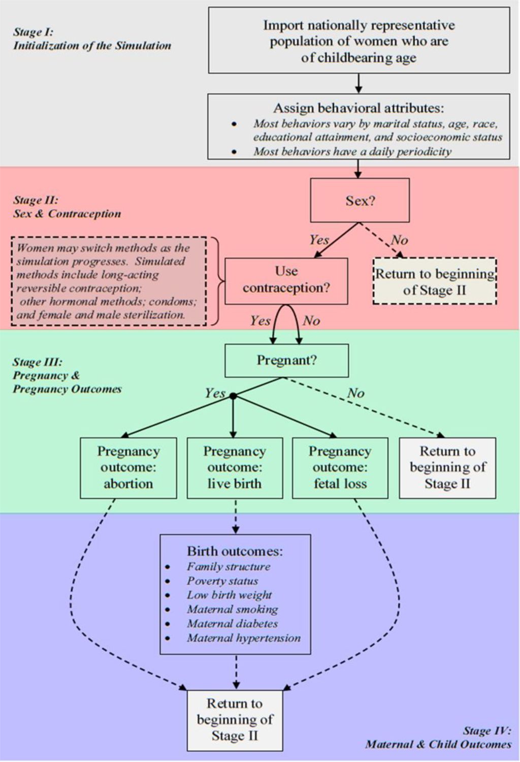
Summary diagram of the FamilyScape 3.0 microsimulation model.

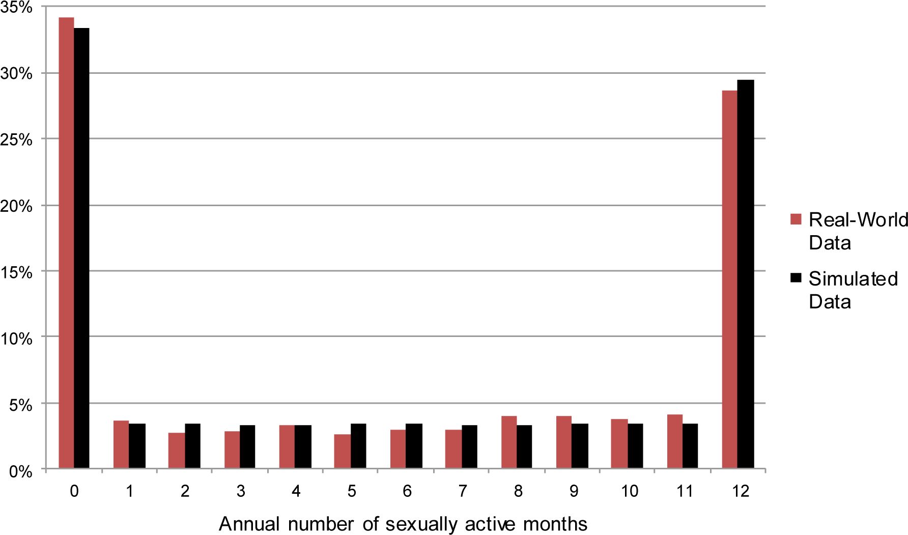
Simulated and real-world annual number of sexually active months, among unmarried women.
Sources: Simulated results were generated using data from 100 one-year steady-state runs of the FamilyScape 3.0 model. Real-world estimates were produced via tabulations of data taken from the female respondent file of the 2006 – 2010 National Survey of Family Growth.
Notes: We do not display confidence intervals because they are so small as to be invisible to the naked eye.

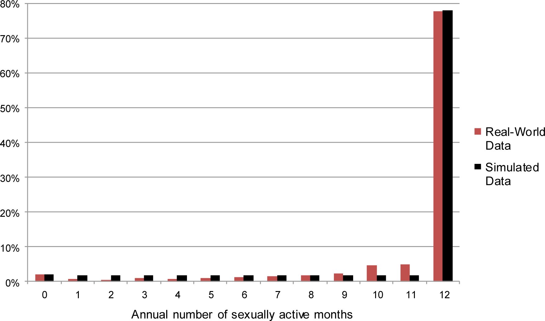
Simulated and real-world annual number of sexually active months, among married women.
Sources: Simulated results were generated using data from 100 one-year steady-state runs of the FamilyScape 3.0 model. Real-world estimates were produced via tabulations of data taken from the female respondent file of the 2006 – 2010 National Survey of Family Growth.
Notes: We do not display confidence intervals because they are so small as to be invisible to the naked eye.
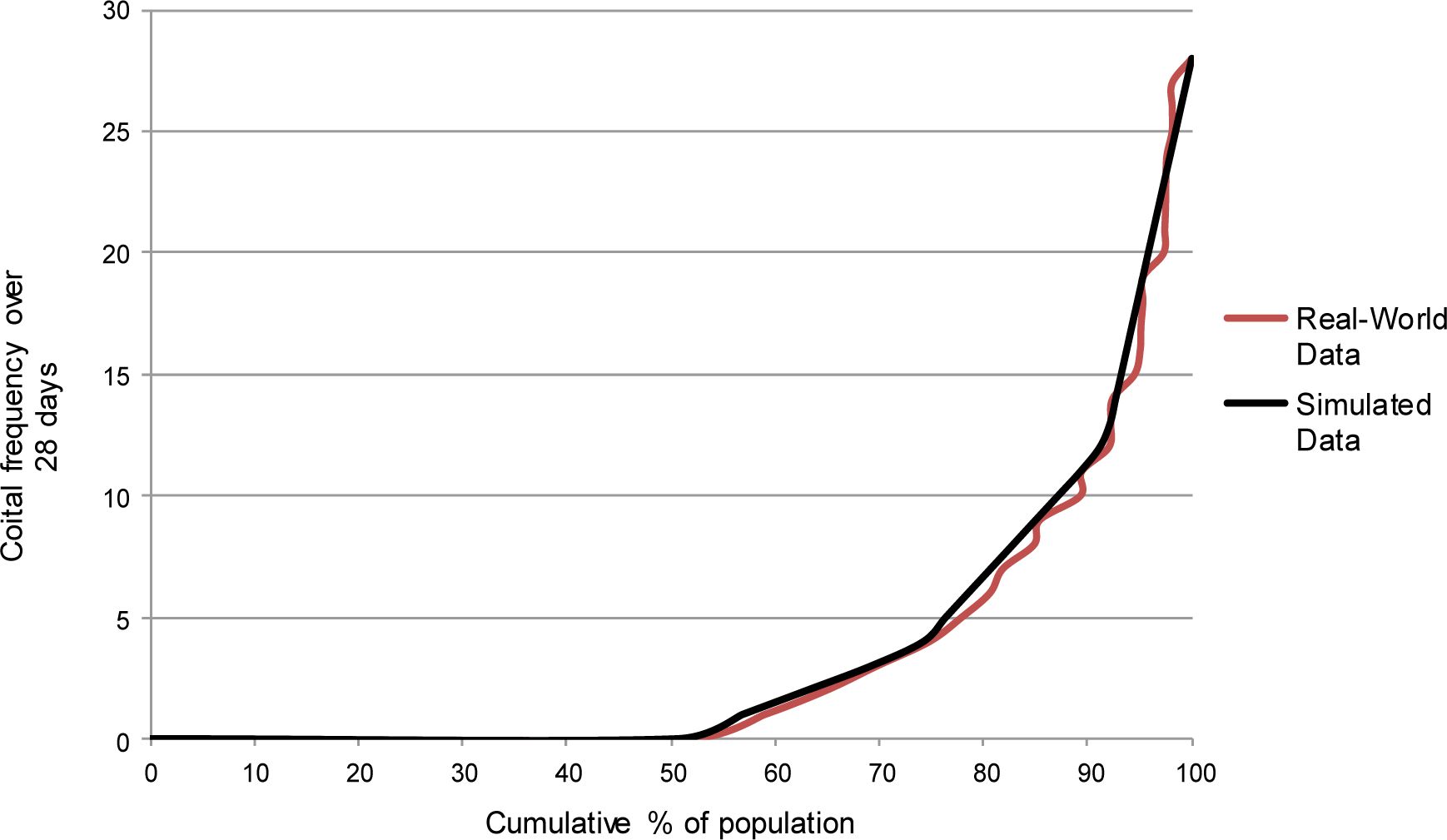
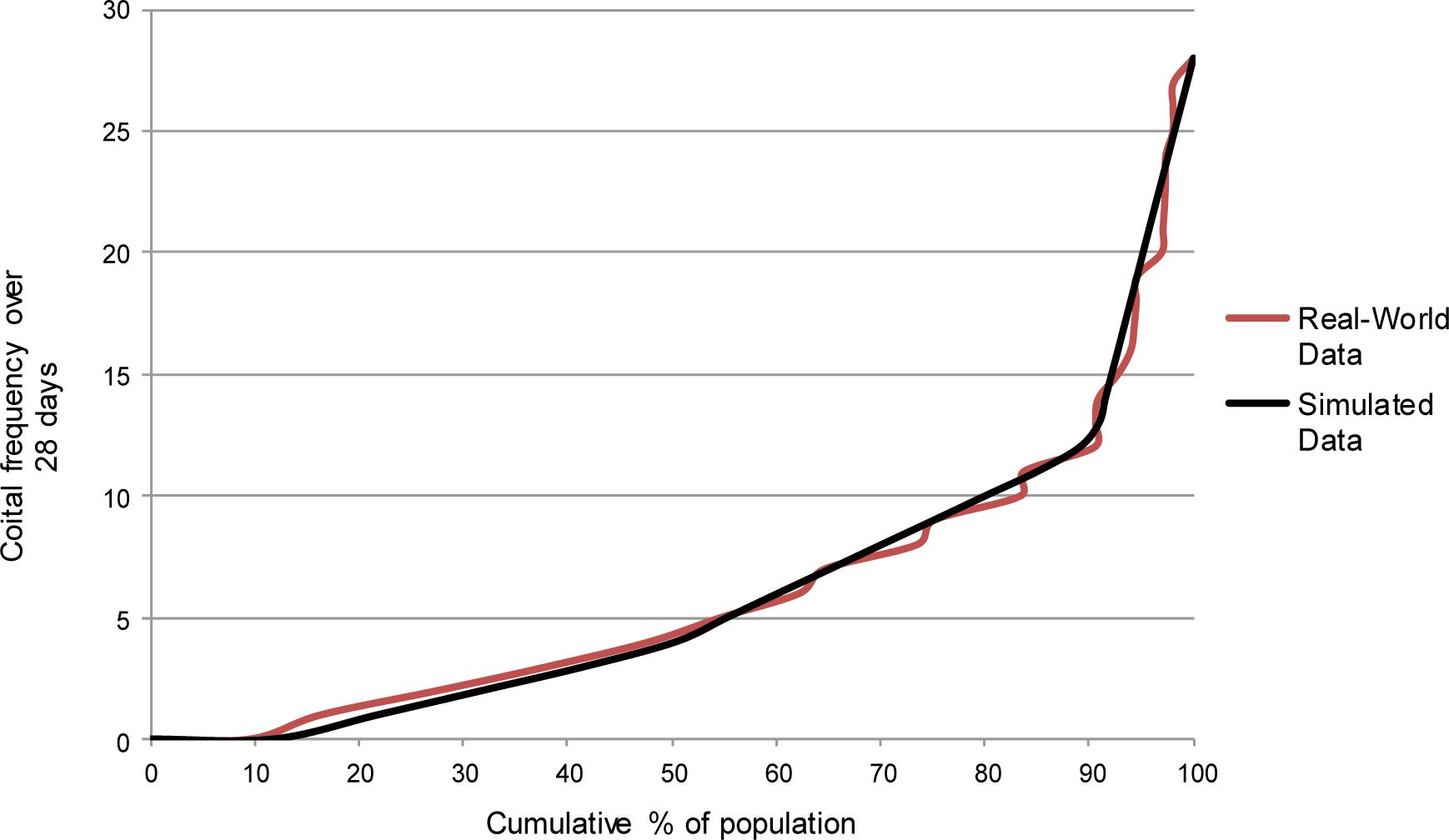
Simulated and real-world within-month coital frequency distributions, among unmarried women.
Sources: Simulated results were generated using data from 100 one-year steady-state runs of the FamilyScape 3.0 model. Real-world estimates were produced via tabulations of data taken from the female respondent file of the 2006 – 2010 National Survey of Family Growth.
Notes: We do not display confidence intervals because they are so small as to be invisible to the naked eye.

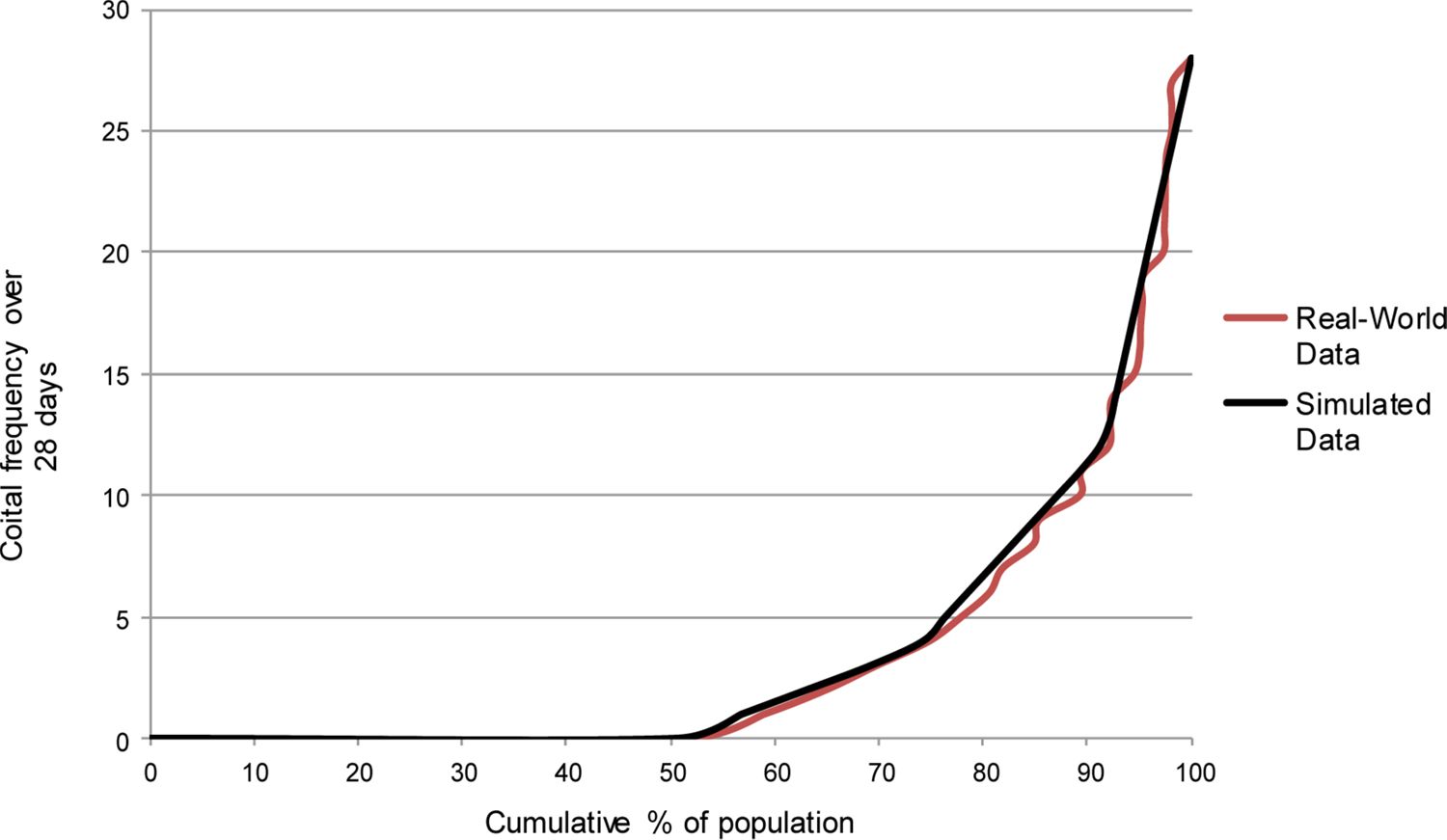
Simulated and real-world within-month coital frequency distributions, among married women.
Sources: Simulated results were generated using data from 100 one-year steady-state runs of the FamilyScape 3.0 model. Real-world estimates were produced via tabulations of data taken from the female respondent file of the 2006 – 2010 National Survey of Family Growth.
Notes: We do not display confidence intervals because they are so small as to be invisible to the naked eye.

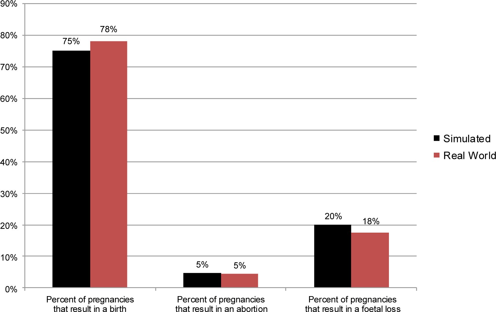
Simulated and real-world pregnancy outcome distributions, among unmarried women.
Sources: Simulated results were generated using data from 100 one-year steady-state runs of the FamilyScape 3.0 model. Real-world estimates were produced via tabulations of data taken from the 2006 – 2010 National Survey of Family Growth and the Guttmacher Institute’s 2008 Abortion Provider Survey.
Notes: We do not display confidence intervals because they are so small as to be invisible to the naked eye.

Simulated and real-world pregnancy outcome distributions, among married women.
Sources: Simulated results were generated using data from 100 one-year steady-state runs of the FamilyScape 3.0 model. Real-world estimates were produced via tabulations of data taken from the 2006 – 2010 National Survey of Family Growth and the Guttmacher Institute’s 2008 Abortion Provider Survey.
Notes: We do not display confidence intervals because they are so small as to be invisible to the naked eye.

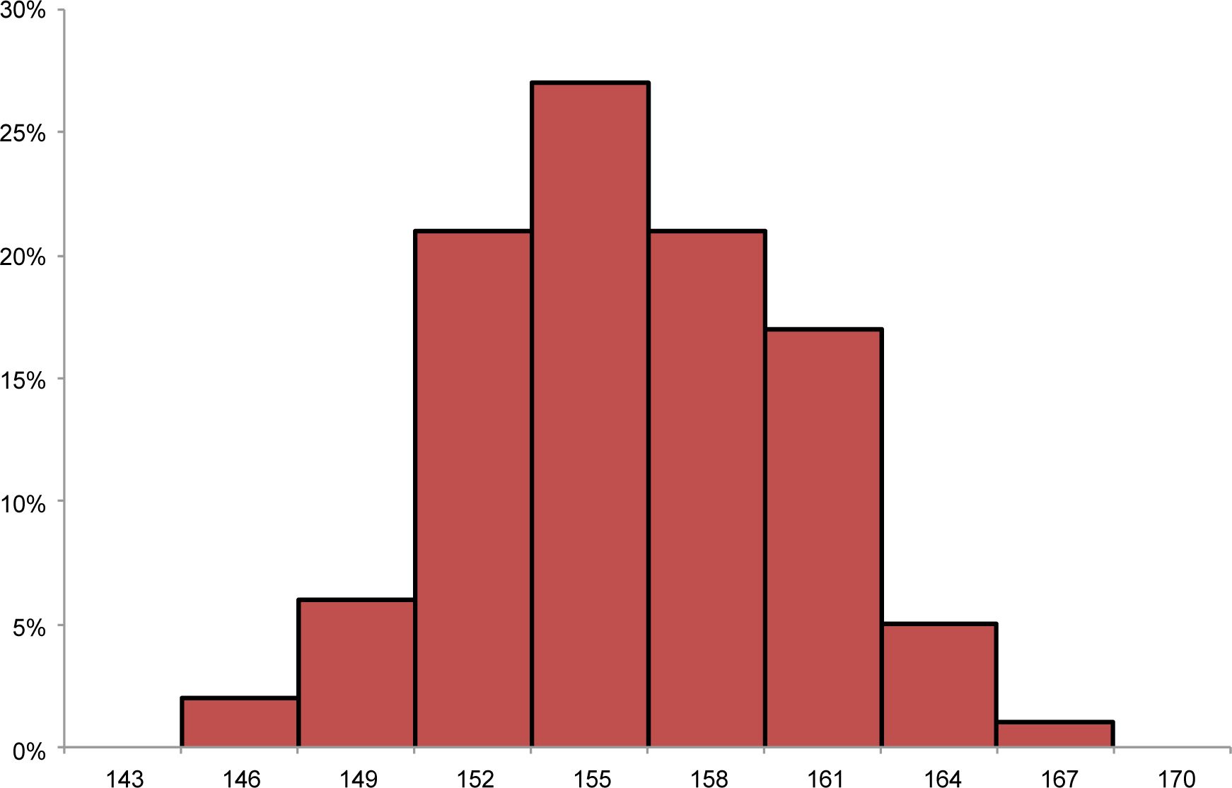
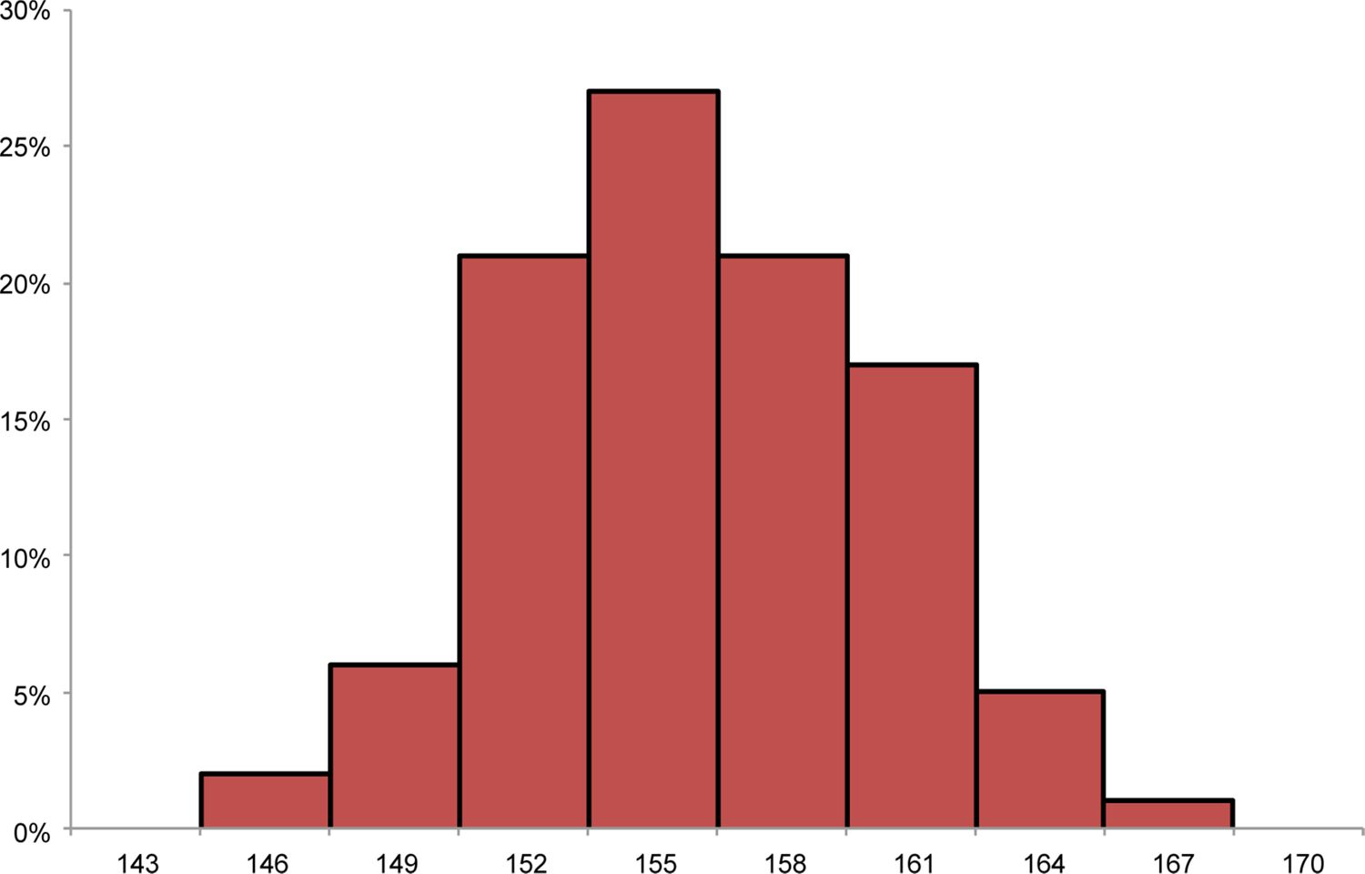
Distribution of annual non-marital pregnancy rates per 1,000 women, across simulation runs.
Source: Results were generated using data from 100 one-year steady-state runs of the FamilyScape 3.0 model.
Distribution of annual marital pregnancy rates per 1,000 women, across simulation runs.
Source: Results were generated using data from 100 one-year steady-state runs of the FamilyScape 3.0 model.
Tables
Specification of FamilyScape’s demographic covariates.
| Covariates | |||||
|---|---|---|---|---|---|
| Categories | Age Group | Race | Educational Attainment | SES | Marital Status |
| 15–19 | White non-Hispanic | Less than high school | Mother had less than a high school degree | Unmarried | |
| 20–24 | Black non-Hispanic | High school degree | Mother had at least a high school degree | Married | |
| 25–29 | Hispanic | More than high school | |||
| 30–44 | Other | ||||
Demographic comparison of the FamilyScape 3.0 simulation population and NSFG respondents.
| Simulation Population | NSFG | |
|---|---|---|
| 15–19 (%) | 16.9% | 17.1% |
| 20–24 (%) | 16.6% | 16.8% |
| 25–29 (%) | 17.6% | 17.1% |
| 30–44 (%) | 49.0% | 49.0% |
| Average age | 29.5 | 29.5 |
| White non-Hispanic (%) | 61.9% | 61.8% |
| Black non-Hispanic (%) | 14.2% | 14.4% |
| Hispanic (%) | 17.3% | 17.0% |
| Other (%) | 6.7% | 6.8% |
| Less than High School (%) | 23.7% | 24.0% |
| High School Degree (%) | 24.7% | 23.8% |
| More than High School (%) | 51.7% | 52.2% |
| Low SES (%) | 22.6% | 22.3% |
| High SES (%) | 77.4% | 77.7% |
| Unmarried (%) | 58.8% | 58.6% |
| Married (%) | 41.2% | 41.4% |
| N | 20,000 | 12,175 |
-
Sources: Simulated results were generated using data from 100 one-year steady-state runs of the FamilyScape 3.0 model. Real-world benchmarks were produced via analysis of the weighted female respondent file of the National Survey of Family Growth 2006–2010.
-
Notes: A woman is considered to be low-SES if her mother had less than a high-school degree.
Simulated and real-world distributions of initial contraceptive type, by marital status.
| Female-Controlled Method (if any) | Male-Controlled Method (if any) | unmarried Women | Married Women |
|---|---|---|---|
| Simulated Data | |||
| None | None | 12.6% (12.5%-12.7%) | 15.5% (15.4%-15.6%) |
| None | Condom | 31.9% (31.8%-32.0%) | 19.4% (19.3%-19.5%) |
| PPR | Nothing | 19.7% (19.6%-19.8%) | 19.8% (19.7%-19.9%) |
| PPR | Condom | 13.9% (13.8%-14.0%) | 3.9% (3.9%-3.9%) |
| LARC | Nothing | 5.6% (5.6%-5.6%) | 6.6% (6.5%-6.7%) |
| LARC | Condom | 1.7% (1.7%-1.7%) | 0.3% (0.3%-0.3%) |
| Any Method Other Than Sterilization | Sterilization | 2.1% (2.1%-2.1%) | 11.7% (11.6%-11.8%) |
| Sterilization | Any Method | 12.6% (12.5%-12.7%) | 22.8% (22.7%-22.9%) |
| Total | 100% | 100% | |
| Real-World Data | |||
| None | None | 11.6% | 15.1% |
| None | Condom | 32.1% | 19.2% |
| PPR | Nothing | 19.4% | 20.0% |
| PPR | Condom | 13.5% | 3.9% |
| LARC | Nothing | 5.9% | 6.7% |
| LARC | Condom | 1.6% | 0.3% |
| Any Method Other Than Sterilization | Sterilization | 2.6% | 11.9% |
| Sterilization | Any Method | 13.3% | 22.9% |
| Total | 100.0% | 100.0% | |
-
Sources: Simulated results were generated using data from 100 one-year steady-state runs of the FamilyScape 3.0 model. Real-world estimates were produced via tabulations of data taken from the National Survey of Family Growth (NSFG) 2006–2010.
-
Notes: Ninety-five percent confidence intervals are reported in parentheses beneath each simulated estimate. Confidence intervals reflect uncertainty related to random variation in simulation results across runs. Simulated estimates indicate initial contraceptive assignment among members of FamilyScape's simulation population. Real-world estimates indicate the most effective couple-level method(s) used in the first sexually active month of the past year among female NSFG respondents.
Simulated and real-world contraceptive switching distributions, among unmarried women.
| Origin Contraceptive Type | Contraceptive-Type Distribution Across Twelve Consecutive Months | ||||||||
|---|---|---|---|---|---|---|---|---|---|
| Female-Controlled Method | Male-Controlled Method | Female Method: Nothing Male Method: Nothing | Female Method: Nothing Male Method: Condom | Female Method: PPR Male Method: Nothing | Female Method: PPR Male Method: Condom | Female Method: LARC Male Method: Nothing | Female Method: LARC Male Method: Condom | Female Method: Anything But Sterilization Male Method: Sterilization | Female Method: Sterilization Male Method: Any Method |
| Simulated Data | |||||||||
| None | None | 88.2% (88.0%–88.3%) | 4.5% (4.4%–4.6%) | 2.6% (2.5%–2.7%) | 0.6% (0.6%–0.7%) | 2.0% (1.9%–2.0%) | 0.1% (0.0%–0.1%) | 0.2% (0.2%–0.3%) | 1.8% (1.8%–1.9%) |
| None | Condom | 3.9% (3.8%–3.9%) | 87.9% (87.8%–88.0%) | 3.2% (3.1%–3.2%) | 2.7% (2.7%–2.8%) | 1.0% (1.0%–1.1%) | 0.3% (0.2%–0.3%) | 0.5% (0.5%–0.5%) | 0.5% (0.5%–0.6%) |
| PPR | None | 2.7% (2.6%–2.7%) | 3.3% (3.2%–3.4%) | 88.8% (88.7%–88.9%) | 3.1% (3.0%–3.1%) | 1.2% (1.1%–1.2%) | 0.1% (0.1%–0.1%) | 0.3% (0.3%–0.3%) | 0.6% (0.5%–0.6%) |
| PPR | Condom | 1.7% (1.6%–1.8%) | 4.2% (4.1%–4.3%) | 6.9% (6.8%–7.0'%) | 85.8% (85.7%–86.0%) | 0.5% (0.5%–0.5%) | 0.4% (0.4%–0.5%) | 0.3% (0.2%–0.3%) | 0.2% (0.2%–0.2%) |
| LARC | None | 4.1% (4.0%–4.3%) | 3.5% (3.3%–3.7%) | 4.6% (4.4%–4.8%) | 0.6% (0.5%–0.6%) | 84.5% (84.2%–84.9%) | 1.4% (1.3%–1.5%) | 0.2% (0.2%–0.3%) | 1.0% (0.9%–1.1%) |
| LARC | Condom | 1.4% (1.3%–1.6%) | 7.2% (6.9%–7.6%) | 2.1% (1.9%–2.3%) | 2.6% (2.3%–2.8%) | 6.0% (5.6%–6.3%) | 79.6% (79.1%–80.2%) | 0.1% (0.1%–0.2%) | 0.9% (0.8%–1.1%) |
| Any Method Other Than Sterilization | Sterilization | 1.6% (1.5%–1.8%) | 3.3% (3. 1 %–3.5 %) | 0.8% (0.7%–0.9%) | 0.5% (0.4%–0.6%) | 0.5% (0.5%–0.6%) | 0.2% (0.1%–0.2%) | 92.3% (92.0%–92.6%) | 0.8% (0.7%–0.9%) |
| Sterilization | Any Method | 0.0% (0.0%–0.0%) | 0.0% (0.0%–0.0%) | 0.0% (0.0%–0.0%) | 0.0% (0.0%–0.0%) | 0.0% (0.0%–0.0%) | 0.0% (0.0%–0.0%) | 0.0% (0.0%–0.0%) | 100% (100.0%–100.0%) |
| Real-World Data | |||||||||
| None | None | 84.9% | 5.9% | 3.6% | 1.2% | 2.4% | 0.3% | 0.6% | 1.1% |
| None | Condom | 3.6% | 88.4% | 3.1% | 3.3% | 0.7% | 0.2% | 0.4% | 0.3% |
| PPR | None | 4.0% | 4.9% | 86.8% | 2.8% | 1.0% | 0.0% | 0.2% | 0.3% |
| PPR | Condom | 1.3% | 4.8% | 8.1% | 84.8% | 0.3% | 0.5% | 0.1% | 0.1% |
| LARC | None | 5.3% | 3.7% | 4.8% | 0.8% | 83.5% | 1.2% | 0.0% | 0.6% |
| LARC | Condom | 0.9% | 8.3% | 1.0% | 3.0% | 5.2% | 81.3% | 0.1% | 0.3% |
| Any Method Other Than Sterilization | Sterilization | 0.6% | 3.5% | 0.7% | 1.6% | 0.1% | 0.0% | 92.9% | 0.6% |
| Sterilization | Any Method | 0.5% | 0.1% | 0.2% | 0.1% | 0.1% | 0.1% | 0.0% | 99.0% |
-
Sources: Simulated results were generated using data from 100 one-year steady-state runs of the FamilyScape 3.0 model. Real-world estimates were produced using data on female members of the National Survey of Family Growth 2006–2010.
-
Notes: Ninety-five percent confidence intervals are reported in parentheses beneath each simulated estimate. Confidence intervals reflect uncertainty related to random variation in simulation results across runs.
Simulated and real-world contraceptive switching distributions, among married women.
| Origin Contraceptive Type | Contraceptive-Type Distribution Across Twelve Consecutive Months | ||||||||
|---|---|---|---|---|---|---|---|---|---|
| Female-Controlled Method | Male-Controlled Method | Female Method: Nothing Male Method: Nothing | Female Method: Nothing Male Method: Condom | Female Method: PPR Male Method: Nothing | Female Method: PPR Male Method: Condom | Female Method: LARC Male Method: Nothing | Female Method: LARC Male Method: Condom | Female Method: Anything But Sterilization Male Method: Sterilization | Female Method: Sterilization Male Method: Any Method |
| Simulated Data | |||||||||
| None | None | 90.6% (90.4%–90.7%) | 2.6% (2.5%–2.6%) | 3.5% (3.4%–3.6%) | 0.3% (0.3%–0.3%) | 1.0% (0.9%–1.0%) | 0.0% (0.0%–0.0%) | 0.7% (0.7%–0.8%) | 1.3% (1.3%–1.4%) |
| None | Condom | 4.3% (4.2%4.4%) | 90.3% (90.2%–90.4%) | 1.8% (1. 7%–1 8%) | 0.5% (0.5%–0.6%) | 0.8% (0.8%–0.9%) | 0.1% (0.1%–0.1%) | 1.2% (1.2%–1.3%) | 0.9% (0.9%–1.0%) |
| PPR | None | 5.3% (5.2%–5.4%) | 3.2% (3.2%–3.3%) | 87.6% (87.5%–87.7%) | 1.2% (1.2%–1.2%) | 0.9% (0.9%–1.0%) | 0.1% (0.1%–0.1%) | 1.0% (0.9%–1.0%) | 0.6% (0.6%–0.6%) |
| PPR | Condom | 3.1% (2.9%–3.3%) | 5.9% (5.7%–6.2%) | 4.5% (4.3%–4.7%) | 84.4% (84.0%–84.7%) | 0.7% (0.6%–0.7%) | 0.1% (0.1%–0.1%) | 1.0% (0.9%–1.0%) | 0.3% (0.3%–0.4%) |
| LARC | None | 1.9% (1.8%–2.0%) | 1.9% (1.8%–1.9%) | 2.2% (2.1%–2.3%) | 0.2% (0.2%–0.3%) | 92.3% (92.1%–92.5%) | 0.2% (0.2%–0.2%) | 0.6% (0.5%–0.6%) | 0.7% (0.7%–0.8%) |
| LARC | Condom | 0.9% (0.6%–1.2%) | 7.2% (6.4%–8.0%) | 0.7% (0.5%–0.9%) | 0.8% (0.6%–1.0%) | 9.5% (8.5 %–10.5 %) | 79.9% (78.5 %–81.3 %) | 0.1% (0.0%–0.3%) | 0.9% (0.7%–1.1%) |
| Any Method Other Than Sterilization | Sterilization | 0.0% (0.0%–0.0%) | 0.0% (0.0%–0.0%) | 0.0% (0.0%–0.0%) | 0.0% (0.0%–0.0%) | 0.0% (0.0%–0.0%) | 0.0% (0.0%–0.0%) | 100% (100.0%–100.0%) | 0.0% (0.0%–0.0%) |
| Sterilization | Any Method | 0.0% (0.0%–0.0%) | 0.0% (0.0%–0.0%) | 0.0% (0.0%–0.0%) | 0.0% (0.0%–0.0%) | 0.0% (0.0%–0.0%) | 0.0% (0.0%–0.0%) | 0.0% (0.0%–0.0%) | 100% (100.0%–100.0%) |
| Real-World Data | |||||||||
| None | None | 88.2% | 3.6% | 4.3% | 0.4% | 1.2% | 0.0% | 0.9% | 1.3% |
| None | Condom | 4.3% | 90.1% | 1.4% | 0.9% | 1.1% | 0.1% | 1.6% | 0.5% |
| PPR | None | 6.8% | 3.5% | 86.5% | 0.7% | 0.8% | 0.0% | 1.2% | 0.6% |
| PPR | Condom | 2.8% | 2.8% | 5.4% | 87.3% | 0.5% | 0.2% | 1.0% | 0.0% |
| LARC | None | 3.2% | 1.8% | 2.6% | 0.2% | 91.2% | 0.1% | 0.6% | 0.4% |
| LARC | Condom | 0.1% | 0.8% | 0.0% | 0.0% | 11.8% | 87.2% | 0.0% | 0.0% |
| Any Method Other Than Sterilization | Sterilization | 0.4% | 0.0% | 0.1% | 0.0% | 0.0% | 0.0% | 98.7% | 0.8% |
| Sterilization | Any Method | 0.2% | 0.1% | 0.0% | 0.0% | 0.0% | 0.0% | 0.1% | 99.5% |
-
Sources: Simulated results were generated using data from 100 one-year steady-state runs of the FamilyScape 3.0 model. Real-world estimates were produced using data on female members of the National Survey of Family Growth 2006–2010.
-
Notes: Ninety-five percent confidence intervals are reported in parentheses beneath each simulated estimate. Confidence intervals reflect uncertainty related to random variation in simulation results across runs.
Simulated and real-world estimates of the proportion of women experiencing a pregnancy within a year of typical use, by contraceptive method.
| Simulated Data | Real-World Data | |
|---|---|---|
| No Method | 66.7% (66.5%–66.9%) | Between 46.0% and 85.0% |
| Condoms | 20.2% (20.1%–20.3%) | 19.0% |
| PPR | 9.6% (9.5%–9.7%) | 9.7% |
| LARC | 3.1% (3.0%–3.2%) | 2.7% |
| Male Sterilization | 0.0% (0.0%–0.0%) | .15% |
| Female Sterilization | 0.0% (0.0%–0.0%) | .5% |
-
Sources: Simulated results were generated using data from 100 one-year steady-state runs of the FamilyScape 3.0 model. Real-world estimates were produced using data taken from Trussell (2011) and Jones et al. (2012).
-
Notes: Ninety-five percent confidence intervals are reported in parentheses beneath each simulated estimate. Confidence intervals reflect uncertainty related to random variation in simulation results across runs.
Simulated and real-world fertility outcomes, by age and marital status.
| Annual Pregnancy Rate (number per 1,000 women | Annual Abortion Rate (number per 1,000 women) | Annual Live Birth Rate (number per 1,000 women) | |||||||
|---|---|---|---|---|---|---|---|---|---|
| Unmarried Women | Married Women | All | Unmarried Women | Married Women | All | Unmarried Women | Married Women | All | |
| Simulated Data | |||||||||
| 15–19 | 78.3 (77.3–79.3) | 215.5 (200.1–230.9) | 79.5 (78.5–80.5) | 19.0 (18.5–19.5) | 45.5 (37.6–53.4) | 19.3 (18.8–19.8) | 45.7 (45.1–46.3) | 126.5 (116.1–136.9) | 46.4 (45.8–47.0) |
| 20–29 | 140.2 (139.1–141.3) | 225.9 (224.1–227.7) | 166.4 (165.4–167.4) | 45.1 (44.5–45.7) | 13.5 (12.9–14.1) | 35.4 (35.0–35.8) | 77.7 (77.0–78.4) | 174.2 (172.7–175.7) | 107.3 (106.7–107.9) |
| 30–39 | 84.0 (82.9–85.1) | 113.9 (112.9–114.9) | 102.8 (102.0–103.6) | 34.1 (33.4–34.8) | 3.8 (3.6–4.0) | 15.1 (14.8–15.4) | 37.6 (36.9–38.3) | 83.6 (82.7–84.5) | 66.5 (65.8–67.2) |
| All | 107.6 (107.0–108.2) | 152.9 (152.1–153.7) | 124.3 (123.8–124.8) | 34.3 (33.9–34.7) | 7.3 (7.1–7.5) | 24.3 (24.1–24.5) | 58.4 (58.0–58.8) | 114.9 (114.2–115.6) | 79.2 (78.8–79.6) |
| Real-World Data | |||||||||
| 15–19 | 67.7 | 234.9 | 72.5 | 19.2 | 0.7 | 18.7 | 37.0 | 194.3 | 41.5 |
| 20–29 | 146.1 | 209.9 | 168.2 | 47.8 | 9.2 | 34.4 | 77.6 | 170.8 | 109.9 |
| 30–39 | 102.1 | 113.6 | 110.0 | 36.2 | 5.5 | 15.2 | 44.8 | 84.7 | 72.2 |
| All | 110.1 | 147.6 | 125.6 | 35.6 | 6.6 | 23.6 | 56.8 | 115.1 | 81.0 |
-
Sources: Simulated results were generated using data from 100 one-year steady-state runs of the FamilyScape 3.0 model. Real-world benchmarks were developed using estimates reported in Zolna and Lindberg (2012), Ventura et al. (2012), and the National Center for Health Statistics' NVSS data resource.
-
Notes: Ninety-five percent confidence intervals are reported in parentheses beneath each simulated estimate. Confidence intervals reflect uncertainty related to random variation in simulation results across runs.
Simulated and real-world maternal and child birth outcomes, by marital status.
| Unmarried Women | Married Women | |
|---|---|---|
| Simulated Data | ||
| Child Poverty | 50.8% (50.4%–51.2%) | 10.2% (10.0%–10.4%) |
| Low Birth Weight | 9.3% (9.1%–9.5%) | 7.0% (6.8%–7.2%) |
| Maternal Smoking | 19.6% (19.3%–19.9%) | 6.1% (5.9%–6.3%) |
| Maternal Diabetes | 3.8% (3.6%–4.0%) | 5.3% (5.1%–5.5%) |
| Maternal Hypertension | 4.3% (4.1%–4.5%) | 4.1% (4.0%–4.2%) |
| Real-World Data | ||
| Child Poverty | 54.5% | 9.9% |
| Low Birth Weight | 9.7% | 7.0% |
| Maternal Smoking | 16.3% | 5.5% |
| Maternal Diabetes | 3.6% | 5.0% |
| Maternal Hypertension | 4.0% | 3.9% |
-
Sources: Simulated results were generated using data from 100 one-year steady-state runs of the FamilyScape 3.0 model. Real-world benchmarks for child poverty were produced via analysis of the March 2009 Current Population Survey. Real-world benchmarks for all other outcomes were produced via analysis of 2008 data from the National Vital Statistics System.
-
Notes: Ninety-five percent confidence intervals are reported in parentheses beneath each simulated estimate. Confidence intervals reflect uncertainty related to random variation in simulation results across runs.
Overview of FamilyScape’s regression specifications.
| Regression Characteristics | Dependent Variable | ||||
|---|---|---|---|---|---|
| Annual Sexual Activity Type | Within-Month Coital Frequency Type | Initial Contraceptive Type | Probability of Switching Contraceptive Types For the first contraceptive switch a | Probability of Switching Contraceptive Types For higher-order contraceptive switchesb | |
| Separate Equations Estimated by Marital Status? | Y | Y | Y | Y | Y |
| Number of Outcomes | 3 | 3 | 8 | 2 | 2 |
| Number of Regressions Estimated for Each Marital-Status Category | 2 | 2 | 7 | 7 (for unmarried women) 6 (for married women) | 1 |
| Functional Form | Logistic Regression | Logistic Regression | Logistic Regression | Logistic Hazard | Logistic Hazard |
| Demographic Covariates: | |||||
| Age | ✓ | ✓ | ✓ | ✓ | ✓ |
| Race | ✓ | ✓ | ✓ | ✓ | ✓ |
| Education | ✓ | ✓ | ✓ | ✓ | ✓ |
| Socioeconomic Status | ✓ | ✓ | ✓ | ✓ | ✓ |
| Behavioral Covariates: | |||||
| Annual Sexual Activity Type | ✓ | ✓ | |||
| Within-Month Coital Frequeny Type | ✓ | ||||
| Pregnant in the Previous Month | ✓ | ✓ | |||
| Number of Previous Contraceptive Switches | ✓ | ||||
| Origin Contraceptive Type | ✓ | ✓ | |||
| Most Recent Contraceptive Type | ✓ | ||||
| Regression Characteristics | Dependent Variable | ||||
| New Contraceptive Type After the first method switch 3 | New Contraceptive Type After higher-order method switches 3 | Pregnancy Outcomes Among women who experience a pregnancy | Probability that a Child will be Born into Poverty Among women whose pregnancy results in a birth | ||
| Separate Equations Estimated by Marital Status? | Y | Y | Y | Y | |
| Number of Outcomes | 8 | 8 | 3 | 2 | |
| Number of Regressions Estimated for Each Marital-Status Category | 7 | 7 | 2 | 1 | |
| Functional Form | Logistic Regression | Logistic Regression | Ordinary Least Squares | Linear Probability Model | |
| Demographic Covariates: | |||||
| Age | ✓ | ✓ | ✓ | ✓ | |
| Race | ✓ | ✓ | ✓ | ✓ | |
| Education | ✓ | ✓ | ✓ | ||
| Socioeconomic Status | ✓ | ✓ | |||
| Behavioral Covariates: | |||||
| Annual Sexual Activity Type | |||||
| Within-Month Coital Frequency Type | |||||
| Pregnant in the Previous Month | ✓ | ✓ | |||
| Number of Previous Contraceptive Switches | ✓ | ||||
| Origin Contraceptive Type | ✓ | ✓ | |||
| Most Recent Contraceptive Type | ✓ | ||||
| Regression Characteristics | Dependent Variable | ||||
| Probability that a Child will be Born at Low Birth Weight Among women whose pregnancy results in a birth | Probability of Maternal Smoking Among women whose pregnancy results in a birth | Probability of Maternal Diabetes Among women whose pregnancy results in a birth | Probability of Maternal Hypertension Among women whose pregnancy results in a birth | ||
| Separate Equations Estimated by Marital Status? | Y | Y | Y | Y | |
| Number of Outcomes | 2 | 2 | 2 | 2 | |
| Number of Regressions Estimated for Each Marital-Status Category | 1 | 1 | 1 | 1 | |
| Functional Form | Logistic Regression | Logistic Regression | Logistic Regression | Logistic Regression | |
| Demographic Covariates: | |||||
| Age | ✓ | ✓ | ✓ | ✓ | |
| Race | ✓ | ✓ | ✓ | ✓ | |
| Education | ✓ | ✓ | ✓ | ✓ | |
| Socioeconomic Status | |||||
| Behavioral Covariates: | |||||
| Annual Sexual Activity Type | |||||
| Within-Month Coital Frequency Type | |||||
| Pregnant in the Previous Month | |||||
| Number of Previous Contraceptive Switches | |||||
| Origin Contraceptive Type | |||||
| Most Recent Contraceptive Type | |||||
-
Notes: All regression models described in this portion of the table were estimated using data on female NSFG respondents.
-
a
For the probability of switching methods for the first time, we estimate separate regressions for each origin contraceptive type except female sterilization (under the simplifying assumption that sterilized women will not undergo surgical reversal of their sterilization) and, for married women, male sterilization (under the simplifying assumptions that each woman who is married to a sterilized man will have the same spouse throughout the simulation and that her spouse will not undergo surgical reversal of his sterilization). All regressions also include a set of monthly baseline hazard dummy variables.
-
b
For higher-order switching, we do not estimate separate equations for each origin contraceptive method because of limited sample sizes. Rather, we estimate one model per marital-status group and include a series of "origin contraceptive type" dummies as covariates. All regressions also include a set of monthly baseline hazard dummy variables.
-
All regression models described in this portion of the table were estimated using data on female NSFG respondents except for: a) the pregnancy-outcome regressions, which additionally use data from the Nationalvital Statistics System and the Guttmacher Institute's Abortion Provider Survey; and b) the child-poverty regressions, which were estimated using Current Population Survey data.
-
c
These regression equations also include a continuous month variable and a quadratic month variable.
Overview of FamilyScape’s non-regression-estimated parameters.
| Dependent Variable | |||
|---|---|---|---|
| Female Fecunditya | Contraceptive Failureb | Gestation Periodsc | |
| Estimation Approach | Equations developed via syntheses of published studies | Original data tabulations | Synthesis of published estimates |
| Covariates | Age, day in menstrual cycle | Marital status, age, contraceptive type | Pregnancy outcome |
-
a
See the main text for a complete listing of the studies whose findings were used to generate FamilyScape's fecundity parameters.
-
b
FamilyScape's contraceptive failure probabilities are generated by plugging parameters that were estimated via analysis of data on female NSFG respondents (e.g., the monthly pregnancy rates and average within-month coital frequencies of women who use a given method, are of a given marital status, and fall into a given age category) into an equation that was developed for the purpose of modelling single-act contraceptive failure rates.
-
c
FamilyScape's gestation periods are extended to account for the period of time after a pregnancy ends during which a woman is infertile. The durations of these post-pregnancy infertility periods, like the gestation periods that precede them, vary according to the pregnancy's outcome. See the main text for a complete listing of the studies whose results were synthesized to generate the model's gestation-period and post-pregnancy-infertility parameters.
Logistic regression results for annual sexual activity, by marital status.
| Inactive | Highly Active | |||
|---|---|---|---|---|
| Unmarried Women | Married Women | Unmarried Women | Married Women | |
| Age:25–29 | −1.021***(.125) | 0.470(.655) | 0.549***(.111) | −0.344(.210) |
| Age:30–44 | −0.447***(.093) | 1.003*(.553) | 0.546***(.100) | −0.055(.190) |
| Education:High School Degree | −0.978***(.101) | −1.334***(.484) | 0.013(.113) | 0.577***(.208) |
| Education:More than High School | −0.752***(.088) | −0.379(.398) | −0.026(.108) | 0.353*(.190) |
| Race:Black | −0.434***(.092) | 0.054(.484) | −0.165*(.099) | −0.140(.180) |
| Race:Hispanic | −0.219**(.104) | −0.332(.471) | 0.021(.117) | 0.271(.186) |
| Race:Other | 0.332**(.164) | 0.498(.681) | 0.046(.207) | −0.385*(.225) |
| High SES | 0.309***(.105) | −0.637(.414) | −0.119(.110) | 0.256*(.151) |
| Pseudo R-Squared | .07 | .03 | .02 | .01 |
| N | 7,989 | 3,675 | 5,431 | 3,588 |
-
Sources: All regressions were estimated using data taken from the 2006 – 2010 National Survey of Family Growth.
-
Notes: Standard errors are reported in parentheses beneath each parameter estimate. One asterisk (*) indicates that the estimate is statistically significant at or beyond the .1 level, two asterisks (**) indicate that the estimate is significant at or beyond the .05 level, and three asterisks (***) indicate that the estimate is significant at or beyond the .01 level.
Logistic regression results for within-month coital frequency, by marital status.
| Low | High | |||
|---|---|---|---|---|
| Unmarried Women | Married Women | Unmarried Women | Married Women | |
| Age:25–29 | 0.058(.129) | 0.415*(.215) | −0.127(.180) | −0.339(.273) |
| Age:30–44 | 0.031(.121) | 0.828***(.197) | −0.280(.184) | −0.277(.247) |
| Education:High School Degree | 0.130(.135) | −0.230(.182) | −0.124(.201) | 0.077(.288) |
| Education:More than High School | −0.109(.123) | −0.353**(.171) | −0.474***(.183) | −0.021(.277) |
| Race:Black | 0.564***(.116) | −0.265(.163) | −0.080(.183) | 0.248(.255) |
| Race:Hispanic | −0.020(.138) | −0.172(.152) | −0.030(.189) | 0.251(.243) |
| Race:Other | −0.010(.241) | 0.311(.221) | −0.020(.385) | −0.441(.493) |
| High SES | −0.359***(.133) | 0.140(.143) | 0.195(.185) | −0.318(.235) |
| Annual Sexual Activity Fixed Effects? | Y | Y | Y | Y |
| Pseudo R-Squared | .05 | .03 | .02 | .02 |
| N | 3,920 | 3,235 | 1,997 | 1,830 |
-
Sources: All regressions were estimated using data taken from the 2006 – 2010 National Survey of Family Growth.
-
Notes: Standard errors are reported in parentheses beneath each parameter estimate. One asterisk (*) indicates that the estimate is statistically significant at or beyond the .1 level, two asterisks (**) indicate that the estimate is significant at or beyond the .05 level, and three asterisks (***) indicate that the estimate is significant at or beyond the .01 level. Each regression includes a set of annual sexual activity fixed effects dummies that measure the number of sexually active months over the course of the focal year.
Logistic regression results for initial contraceptive assignment, among unmarried women.
| No Method | Condom Only | PPR Only | PPR & Condom | LARC Only | LARC & Condom | Male Sterilization | |
|---|---|---|---|---|---|---|---|
| Age: 25–29 | −1.953***(.386) | −1.085***(.185) | −0.285*(.172) | −0.775***(.206) | 0.180(.201) | −0.473(.616) | 0.786(.707) |
| Age: 30–44 | −3.222***(.353) | −2.188***(.171) | −0.508***(.176) | −1.108***(.219) | −0.660***(.241) | −1.345**(.628) | 2.462***(.493) |
| Education: High School Degree | 0.082(.285) | 0.076(.187) | 0.626***(.209) | 0.563**(.242) | −0.077(.228) | −0.010(.406) | 1.360**(.583) |
| Education: More than High School | 0.584*(.314) | 0.954***(.181) | 1.089***(.192) | 1.084***(.205) | −0.606***(.212) | −0.504(.393) | 1.003*(.550) |
| Race: Black | 0.465(.283) | −0.280(.173) | −1.349***(.170) | −0.727***(.203) | 0.607***(.229) | 0.865**(.392) | −3.595***(.747) |
| Race: Hispanic | 0.635*(.337) | 0.059(.195) | −0.251(.189) | −0.541**(.264) | 0.718***(.229) | 0.245(.557) | −0.573(.622) |
| Race: Other | 0.811(.777) | −0.144(.363) | 0.006(.296) | −0.827**(.356) | −0.355(.396) | 0.205(1.137) | −1.221(1.028) |
| High SES | 0.164(.276) | 0.261(.170) | 0.274(.186) | 0.500*(.267) | −0.379*(.212) | 0.240(.438) | 0.405(.576) |
| Sexual Behavior Fixed Effects? | Y | Y | Y | Y | Y | Y | Y |
| Pseudo R-Squared | .23 | .21 | .13 | .10 | .07 | .06 | .20 |
| N | 989 | 2,247 | 2,969 | 3,439 | 3,732 | 3,812 | 3,885 |
-
Sources: All regressions were estimated using data taken from the 2006 – 2010 National Survey of Family Growth.
-
Notes: Standard errors are reported in parentheses beneath each parameter estimate. One asterisk (*) indicates that the estimate is statistically significant at or beyond the .1 level, two asterisks (**) indicate that the estimate is significant at or beyond the .05 level, and three asterisks (***) indicate that the the .01 level. Each regression includes a set of sexual behaviour fixed effects dummies that reflect interactions between annual sexual activity type and within-month coital frequency type.
Logistic regression results for initial contraceptive assignment, among married women.
| No Method | Condom Only | PPR Only | PPR & Condom | LARC Only | LARC & Condom | Male Sterilization | |
|---|---|---|---|---|---|---|---|
| Age: 25–29 | −0.770*(.454) | −0.777***(.272) | −0.664***(.232) | 0.146(.422) | −0.140(.310) | −0.566(1.255) | 1.639***(.602) |
| Age: 30–44 | −2.038***(.426) | −1.444***(.245) | −1.334***(.215) | −0.136(.408) | −0.353(.284) | −0.789(1.196) | 3.326***(.550) |
| Education: High School Degree | 0.648**(.289) | 0.182(.246) | 0.059(.252) | 0.293(.607) | 0.046(.295) | -- | 1.039***(.383) |
| Education: More than High School | 1 251***(.259) | 0.887***(.226) | 1.170***(.223) | 1.176*(.522) | −0.086(.260) | -- | 0.862**(.365) |
| Race: Black | 0.035(.238) | −0.553**(.242) | −0.425*(.234) | −0.550(.454) | 0.578*(.298) | -- | −1.712***(.385) |
| Race: Hispanic | 0.112(.245) | 0.322*(.195) | −0.077(.184) | −0.086(.358) | 0.329(.232) | -- | −0.412(.266) |
| Race: Other | 0.788**(.400) | 0.870***(.294) | −1.348***(.296) | 0.044(.384) | 0.627*(.354) | -- | −0.772*(.434) |
| High SES | 0.105(.219) | 0.120(.192) | 0.166(.183) | −0.377(.295) | −0.122(.232) | -- | 0.236(.218) |
| Sexual Behavior Fixed Effects? | Y | Y | Y | Y | Y | Y | Y |
| Pseudo R-Squared | .11 | .07 | .09 | .03 | .02 | .01 | .10 |
| N | 1,189 | 1,833 | 2,483 | 2,612 | 2,858 | 2,869 | 3,205 |
-
Sources: All regressions were estimated using data taken from the 2006 – 2010 National Survey of Family Growth.
-
Notes: Standard errors are reported in parentheses beneath each parameter estimate. One asterisk (*) indicates that the estimate is statistically significant at or beyond the .1 level, two asterisks (**) indicate that the estimate is significant at or beyond the .05 level, and three asterisks (***) indicate that the estimate is significant at or beyond the .01 level. Each regression includes a set of sexual behaviour fixed effects dummies that reflect interactions between annual sexual activity type and within-month coital frequency type.
Logistic hazard regression results for the probability of a first method switch, among unmarried women.
| Origin Contraceptive Type | |||||||
|---|---|---|---|---|---|---|---|
| No Method | Condom Only | PPR Only | PPR & Condom | LARC Only | LARC & Condom | Male Sterilization | |
| Age: 25–29 | −0.274*(.146) | −0.282***(.106) | −0.253**(.117) | 0.144(.166) | −0.715***(.183) | −0.711(.471) | 1.336(.924) |
| Age: 30–44 | −0.803***(.155) | −0.299***(.104) | −0.529***(.136) | 0.063(.193) | −0.752***(.236) | 0.062(.456) | 1.263(.983) |
| Education: High School Degree | 0.227(.146) | −0.098(.105) | −0.428***(.161) | −0.504***(.191) | −0.618***(.213) | −0.680*(.394) | −2.601**(1.111) |
| Education: More than High School | 0.485***(.155) | 0.004(.097) | 0.364**(.148) | −0.958***(.171) | −0.468**(.202) | −0.630*(.339) | −1.014(.723) |
| Race: Black | −0.268*(.139) | −0.272***(.095) | 0.595***(.126) | 0.194(.160) | 0.049(.208) | −0.896***(.296) | 1.487*(.803) |
| Race: Hispanic | 0.132(.156) | −0.074(.104) | −0.104(.158) | 0.179(.228) | 0.511(.239) | −0.358(.427) | −0.033(1.007) |
| Race: Other | −0.388(.289) | −0.345*(.195) | −0.131(.234) | 0.405(.341) | 0.630*(.369) | 0.013(.674) | 0.295(1.116) |
| High SES | 0.177(.137) | −0.019(.100) | −0.148(.158) | 0.061(.206) | −0.039(.206) | 0.287(.340) | −0.831(.885) |
| Pregnant Last Month | 2.138***(.197) | 2.38***(.232) | 2.775***(.357) | 2.96***(.524) | 3.69***(.739) | -- | -- |
| Pseudo R-Squared | .08 | .03 | .03 | .04 | .06 | .09 | .09 |
| N | 13,625 | 34,117 | 24,711 | 12,347 | 7,406 | 1,959 | 2,185 |
-
Sources: All regressions were estimated using data taken from the 2006 – 2010 National Survey of Family Growth.
-
Notes: Standard errors are reported in parentheses beneath each parameter estimate. One asterisk (*) indicates that the estimate is statistically significant at or beyond the .1 level, two asterisks (**) indicate that the estimate is significant at or beyond the .05 level, and three asterisks (***) indicate that the estimate is significant at or beyond the .01 level.
Logistic hazard regression results for the probability of a first method switch, among married women.
| Origin Contraceptive Type | ||||||
|---|---|---|---|---|---|---|
| No Method | Condom Only | PPR Only | PPR & Condom | LARC Only | LARC & Condom | |
| Age: 25–29 | −0.341(.208) | −0.254(.205) | −0.009(.147) | −0.062(.300) | −0.559*(.316) | −0.346(1.006) |
| Age: 30–44 | −0.772***(.181) | −0.441**(.187) | −0.359***(.139) | −0.617**(.306) | −1.121***(.321) | −3.254***(.934) |
| Education: High School Degree | −0.249(.234) | 0.065(.244) | −0.146(.242) | −0.434(.643) | −0.682**(.308) | -- |
| Education: More than High School | 0.090(.217) | 0.347*(.211) | −0.216(.232) | −0.718(.665) | −0.299(.298) | -- |
| Race: Black | −0.364*(.204) | −0.403*(.241) | −0.006(.187) | −0.596(.534) | −0.364(.417) | -- |
| Race: Hispanic | −0.047(.197) | 0.386**(.183) | −0.270(.185) | −1.027(.660) | 0.164(.350) | -- |
| Race: Other | −0.564*(.305) | −0.951***(.242) | 0.278(.238) | −1.450***(.533) | 0.170(.421) | -- |
| High SES | −0.032(.178) | −0.018(.177) | 0.031(.169) | −.333(.521) | −0.226(.341) | -- |
| Pregnant Last Month | 3.180***(.200) | 3.348***(.390) | 3.167***(.432) | 2.621***(.720) | -- | -- |
| Pseudo R-Squared | .13 | .06 | .02 | .10 | .04 | .27 |
| N | 17,420 | 20,182 | 21,830 | 3,749 | 7,949 | 220 |
-
Sources: All regressions were estimated using data taken from the 2006 – 2010 National Survey of Family Growth.
-
Notes: Standard errors are reported in parentheses beneath each parameter estimate. One asterisk (*) indicates that the estimate is statistically significant at or beyond the .1 level, two asterisks (**) indicate that the estimate is significant at or beyond the .05 level, and three asterisks (***) indicate that the estimate is significant at or beyond the .01 level.
Logistic hazard regression results for the probability of a higher-order method switch, by marital status.
| Unmarried Women | Married Women | |
|---|---|---|
| Age: 25–29 | −0.049(.074) | −0.169(.141) |
| Age: 30–44 | 0.029(.086) | −0.194(.138) |
| Education: High School Degree | −0.084(.083) | 0.127(.210) |
| Education: More than High School | −0.171**(.079) | 0.187(.197) |
| Race: Black | −0.022(.072) | 0.040(.183) |
| Race: Hispanic | 0.049(.087) | 0.250(.154) |
| Race: Other | −0.370**(.161) | 0.028(.214) |
| High SES | 0.045(.079) | 0.045(.137) |
| Pregnant Last Month | 1.940***(.177) | 2.898***(.214) |
| Number of Previous Switches | 0.531***(.038) | 0.416***(.077) |
| Origin Contraceptive Type Fixed Effects? | Y | Y |
| Most Recent Contraceptive Type Fixed Effects? | Y | Y |
| Pseudo R-Squared | .08 | .12 |
| N | 21,405 | 9,559 |
-
Sources: All regressions were estimated using data taken from the 2006 – 2010 National Survey of Family Growth.
-
Notes: Standard errors are reported in parentheses beneath each parameter estimate. One asterisk (*) indicates that the estimate is statistically significant at or beyond the .1 level, two asterisks (**) indicate that the estimate is significant at or beyond the .05 level, and three asterisks (***) indicate that the estimate is significant at or beyond the .01 level. Each regression includes a set of fixed effects dummies that control for origin contraceptive type and most recent contraceptive type.
Logistic regression results for method selection after a first method switch, among unmarried women.
| Dependent Variable: New Contraceptive Type | |||||||
|---|---|---|---|---|---|---|---|
| Condom Only | PPR Only | PPR & Condom | LARC Only | LARC & Condom | Male Sterilization | Female Sterilization | |
| Age: 25–29 | −0.506**(.230) | −0.027(.165) | −0.537***(.174) | −0.020(.231) | −0.164(.350) | 1.182**(.520) | 1.516***(.383) |
| Age: 30–44 | −0.321(.270) | −0.231(.175) | −0.901***(.223) | −0.188(.267) | −0.401(.312) | 2.653***(.406) | 2.441***(.333) |
| Education: High School Degree | 0.303(.264) | −0.118(.179) | 0.191(.207) | −0.214(.227) | −0.117(.343) | 0.904(.552) | 0.140(.338) |
| Education: More than High School | 0.907***(.260) | 0.143(.169) | 0.968***(.188) | −0.189(.238) | −0.399(.323) | 0.255(.520) | −0.269(.351) |
| Race: Black | −0.259(.243) | −0.646***(.158) | −0.567***(.177) | 0.073(.200) | 0.846***(.273) | −2.218***(.494) | −0.698**(.300) |
| Race: Hispanic | −0.036(.253) | 0.101(.189) | −0.338*(.201) | 0.072(.254) | −0.147(.447) | −0.694*(.388) | −0.185(.365) |
| Race: Other | −0.321(.422) | 0.499*(.301) | −0.469(.353) | −0.073(.463) | 0.352(.505) | −0.562(.920) | .043(.556) |
| High SES | 0.508**(.254) | 0.381**(.180) | 0.340*(.207) | −0.331(.241) | 0.043(.326) | 0.884**(.412) | −0.462(.293) |
| Pregnant Last Month | −1.96***(.556) | 0.311(.303) | −0.485(.428) | 1.268***(,327) | −0.856(.597) | -- | 1 244***(.363) |
| Number of Months at Risk Of First Switch | −0.087(.144) | 0.074(.102) | −0.051(.106) | −0.015(.126) | −0.156(.176) | .0536(.268) | 0.019(.201) |
| Number of Months at Risk Of First Switch Squared | 0.006(.011) | −0.006(.008) | −0.004(.008) | −0.001(.001) | 0.009(.013) | −0.003(.019) | 0.000(.016) |
| Origin Contraceptive Type Fixed Effects? | Y | Y | Y | Y | Y | Y | Y |
| Pseudo R-Squared | .11 | .05 | .14 | .09 | .12 | .20 | .20 |
| N | 1,140 | 2,361 | 3,056 | 3,735 | 4,016 | 3,978 | 4,399 |
-
Sources: All regressions were estimated using data taken from the 2006 – 2010 National Survey of Family Growth.
-
Notes: Standard errors are reported in parentheses beneath each parameter estimate. One asterisk (*) indicates that the estimate is statistically significant at or beyond the .1 level, two asterisks (**) indicate that the estimate is significant at or beyond the .05 level, and three asterisks (***) indicate that the estimate is significant at or beyond the .01 level. Each regression includes a set of fixed effects dummies that that control for origin contraceptive type.
Logistic regression results for method selection after a first method switch, among married women.
| Dependent Variable: New Contraceptive Type | |||||||
|---|---|---|---|---|---|---|---|
| Condom Only | PPR Only | PPR & Condom | LARC Only | LARC & Condom | Male Sterilization | Female Sterilization | |
| Age: 25–29 | −0.878***(.299) | −0.243(.267) | −0.120(.339) | −0.316(.328) | −1.079(1.036) | 0.519(.891) | 0.489(.430) |
| Age: 30–44 | −0.341(.286) | −0.606**(.266) | −0.129(.327) | −0.040(.303) | −1.171(.953) | 2.229***(.851) | 1.539***(.359) |
| Education: High School Degree | 0.876*(.045) | 0.255(.367) | 1.249**(.612) | −1.184***(.365) | −0.443(1.145) | 0.493(.625) | −0.441(.418) |
| Education: More than High School | 0.669(.418) | 0.368(.341) | 1.225**(.554) | −0.958***(.309) | −0.552(1.241) | 0.217(.560) | −1.273***(.428) |
| Race: Black | −0.524(.467) | 0.388(.318) | −0.273(.474) | −0.099(.528) | 0.036(.947) | −0.876(.648) | 0.446(.403) |
| Race: Hispanic | 0.361(.335) | −0.120(.307) | −0.386(.382) | 0.435(.286) | −1.154*(.692) | −0.185(.396) | 0.763**(.384) |
| Race: Other | −0.318(.527) | −0.185(.347) | −0.920**(.439) | 0.144(.486) | −1.394(1.124) | −0.077(.604) | 0.663(.475) |
| High SES | −0.411(.298) | −0.256(.280) | −0.323(.326) | −0.017(.283) | 0.859(.657) | 0.462(.402) | 0.351(.370) |
| Pregnant Last Month | −0.130(.682) | −0.344(.326) | −0.578(.556) | 0.116(.352) | 2.603***(.877) | −2.954***(.851) | 0.754**(.361) |
| Number of Months at Risk Of First Switch | 0.029(.180) | −0.151(.147) | 0.015(.194) | −0.012(.188) | −0.513(.490) | 0.438*(.231) | −0.017(.192) |
| Number of Months at Risk Of First Switch Squared | −0.003(.014) | 0.009(.012) | −0.006(.015) | 0.001(.015) | 0.033(.036) | −0.034**(.017) | 0.008(.014) |
| Origin Contraceptive Type Fixed Effects? | Y | Y | Y | Y | Y | Y | Y |
| Pseudo R-Squared | .06 | .10 | .05 | .06 | .23 | .12 | .14 |
| N | 754 | 1,000 | 1,584 | 1,710 | 1,880 | 1,999 | 2,144 |
-
Sources: All regressions were estimated using data taken from the 2006 – 2010 National Survey of Family Growth.
-
Notes: Standard errors are reported in parentheses beneath each parameter estimate. One asterisk (*) indicates that the estimate is statistically significant at or beyond the .1 level, two asterisks (**) indicate that the estimate is significant at or beyond the .05 level, and three asterisks (***) indicate that the estimate is significant at or beyond the .01 level. Each regression includes a set of fixed effects dummies that that control for origin contraceptive type.
Logistic regression results for method selection after a higher-order method switch, among unmarried women.
| Dependent Variable: New Contraceptive Type | |||||||
|---|---|---|---|---|---|---|---|
| Condom Only | PPR Only | PPR & Condom | LARC Only | LARC & Condom | Male Sterilization | Female Sterilization | |
| Age: 25–29 | 0.128(.373) | 0.002(.198) | 0.250(.242) | 0.349(.269) | 0.158(.433) | 1.142*(.640) | 1.198**(.577) |
| Age: 30–44 | −0.024(.451) | 0.117(.256) | −0.336(.276) | −0.167(.293) | 0.008(.401) | 2.74**(.620) | 1.536**(.499) |
| Education: High School Degree | −0.962**(.338) | 0.163(.238) | −0.071(.277) | −0.289(.331) | 0.067(.505) | −0.155(.527) | −0.059(.482) |
| Education: More than High School | −0.032(.344) | 0.193(.234) | 0.965**(.239) | −0.916**(.279) | −0.370(.536) | −0.233(.505) | −0.685(.458) |
| Race: Black | −0.552*(.310) | −0.849**(.202) | −0.742**(.212) | −0.600(.244) | 0.732**(.315) | −2.101**(.850) | −0.213(.604) |
| Race: Hispanic | −0.450(.357) | −0.088(.242) | −0.093(.279) | 0.012(.300) | 0.542(.594) | −0.676(.703) | −0.051(.491) |
| High SES | 0.150(.329) | −0.061(.225) | 0.017(.257) | −0.026(.275) | 0.236(.448) | 0.674(.841) | 0.216(.483) |
| Pregnant Last Month | −1.338*(.789) | 1.436**(.300) | −0.732(.559) | 0.553(.349) | 0.713(.703) | −2.212**(1.115) | 1.242**(.453) |
| Number of Previous Switches | −0.172(.186) | 0.143*(.082) | 0.112(.088) | −0.069(.152) | −0.046(.210) | −0.030(.314) | −0.291(.210) |
| Number of Months at Risk Of Higher-Order Switch | −0.076(.230) | −0.066(.159) | 0.078(.173) | 0.133(.209) | −0.016(.377) | 0.359(.478) | 0.600**(.286) |
| Number of Months at Risk Of Higher-Order Switch Squared | −0.001(.019) | 0.000(.013) | −0.010(.015) | −0.016(.019) | 0.011(.036) | −0.028(.037) | −0.046**(.022) |
| Most Recent Contraceptive Type Fixed Effects? | Y | Y | Y | Y | Y | Y | Y |
| Origin Contraceptive Type Fixed Effects? | Y | Y | Y | Y | Y | Y | Y |
| Pseudo R-Squared | .26 | .23 | .25 | .25 | .36 | .27 | .12 |
| N | 735 | 1,839 | 2,078 | 2,791 | 2,901 | 3,014 | 3,107 |
-
Sources: All regressions were estimated using data taken from the 2006 – 2010 National Survey of Family Growth.
-
Notes: Standard errors are reported in parentheses beneath each parameter estimate. One asterisk (*) indicates that the estimate is statistically significant at or beyond the .1 level, two asterisks (**) indicate that the estimate is significant at or beyond the .05 level, and three asterisks (***) indicate that the estimate is significant at or beyond the .01 level. Each regression includes two sets of fixed effects dummies, one of which controls for origin contraceptive type and the other of which controls for most recent contraceptive type.
Logistic regression results for method selection after a higher-order method switch, among married women.
| Dependent Variable: New Contraceptive Type | |||||||
|---|---|---|---|---|---|---|---|
| Condom Only | PPR Only | PPR & Condom | LARC Only | LARC & Condom | Male Sterilization | Female Sterilization | |
| Age: 25–29 | −0.314(.617) | −0.329(.457) | −0.585(.601) | −0.153(.471) | −1.869*(.942) | -- | 1.603(1.002) |
| Age: 30–44 | 0.598(.653) | 0.212(.472) | −0.088(.597) | −0.493(.479) | −2.768***(.584) | -- | 2.255**(.967) |
| Education: High School Degree | 0.227(.736) | 0.606(.568) | 0.200(.895) | −0.015(.585) | 2.493*(1.332) | -- | 1.415*(.778) |
| Education: More than High School | 0.992(.769) | 0.317(.529) | 1.159(.905) | −0.813(.548) | 3.021***(1.082) | -- | −0.408(.748) |
| Race: Black | 0.872(.696) | −0.998*(.580) | 0.921(.635) | 1.756***(.490) | 3.653***(1.117) | -- | 1.016(.692) |
| Race: Hispanic | 1.192(.905) | 0.080(.405) | 0.280(.695) | 0.294(.456) | −0.688(.926) | -- | −0.876(.689) |
| High SES | 1.122(.778) | 0.411(.374) | −0.892(.593) | −0.945**(.427) | −3.741***(.835) | -- | −0.511(.735) |
| Pregnant Last Month | −0.133(1.612) | −0.608(.446) | 0.688(.660) | −0.224(.485) | 1.012(1.322) | 0.279(.866) | 0.580(.584) |
| Number of Previous Switches | 0.802(.632) | 0.331*(.198) | 0.541*(.279) | −0.191(.300) | 1 451***(.540) | −0.647(.510) | −1.643*(.903) |
| Number of Months at Risk Of Higher-Order Swi tch | 0.609(.541) | 0.119(.272) | 0.055(.351) | −0.405(.350) | 1.695***(.643) | 0.(.461) | −0.256(..528) |
| Number of Months at Risk Of Higher-Order Swi tch Squared | −0.079*(.042) | −0.027(.024) | −0.017(.031) | 0.042(.030) | −0.196***(.069) | −0.003(.038) | 0.029(.043) |
| Most Recent Contraceptive Type Fixed Effects? | Y | Y | Y | Y | Y | Y | Y |
| Origin Contraceptive Type Fixed Effects? | Y | Y | Y | Y | Y | Y | Y |
| Pseudo R-Squared | .37 | .22 | .28 | .29 | .46 | .16 | .29 |
| N | 167 | 582 | 648 | 846 | 867 | 914 | 950 |
-
Sources: All regressions were estimated using data taken from the 2006 – 2010 National Survey of Family Growth.
-
Notes: Standard errors are reported in parentheses beneath each parameter estimate. One asterisk (*) indicates that the estimate is statistically significant at or beyond the .1 level, two asterisks (**) indicate that the estimate is significant at or beyond the .05 level, and three asterisks (***) indicate that the estimate is significant at or beyond the .01 level. Each regression includes two sets of fixed effects dummies, one of which controls for origin contraceptive type and the other of which controls for most recent contraceptive type.
Pregnancy outcome regression results, by marital status.
| Abortion | Live Birth | |||
|---|---|---|---|---|
| Unmarried Women | Married Women | Unmarried Women | Married Women | |
| Age: 20–24 | 0.046***(.001) | −0.125***(.003) | −0.005***(.001) | 0144***(.002) |
| Age: 25–29 | 0.095***(.001) | −0.169***(.003) | −0.040***(.001) | 0.192***(.002) |
| Age: 30–44 | 0.164***(.001) | −0.187***(.003) | −0.139***(.001) | 0.142***(.002) |
| Race: Black | 0.076***(.001) | 0.073***(.001) | −0.078***(.001) | −0.119***(.000) |
| Race: Hispanic | −0.087***(.001) | 0.025***(.001) | 0.082***(.001) | 0.003***(.000) |
| Race: Other | 0.004***(.001) | 0.034***(.001) | −0.003***(.001) | −0.031***(.000) |
| Constant | 0.245***(.001) | 0.204***(.003) | 0.585***(.001) | 0.606***(.002) |
| R-Squared | .97 | .93 | .98 | .98 |
| N | 2,929 | 2,046 | 2,929 | 2,046 |
-
Sources: All regressions were estimated using data on members of FamilyScape’s simulation population.
-
Notes: Standard errors are reported in parentheses beneath each parameter estimate. One asterisk (*) indicates that the estimate is statistically significant at or beyond the .1 level, two asterisks (**) indicate that the estimate is significant at or beyond the .05 level, and three asterisks (***) indicate that the estimate is significant at or beyond the .01 level. For each ordinary least squares regression, the dependent variable is the probability (ranging from 0 to 1) that a pregnancy will result in a given outcome. See the main text for more information on the data and methods that were used to parameterize FamilyScape’s pregnancy-outcomes module.
Birth outcome regression results, by marital status.
| Child Poverty | Low Birth Weight | Maternal Smoking | Maternal Diabetes | Maternal Hypertension | ||||||
|---|---|---|---|---|---|---|---|---|---|---|
| Unmarried Women | Married Women | Unmarried Women | Married Women | Unmarried Women | Married Women | Unmarried Women | Married Women | Unmarried Women | Married Women | |
| Age: 20–24 | 0.115(.076) | −0.030(.118) | −0.070***(.009) | −0.179***(.021) | 0.597***(.009) | 0.054***(.020) | 0.616***(.020) | 0.599***(.040) | −0.198***(.014) | −0.110***(.029) |
| Age: 25–29 | 0.074(.081) | −0.076(.116) | −0.032***(.010) | −0.222***(.020) | 0.747***(.010) | −0.295***(.020) | 1.190***(.020) | 1.057***(.039) | −0.216***(.015) | −0.157***(.028) |
| Age: 30–44 | 0.113(.083) | −0.082(.116) | 0.187***(.010) | −0.050**(.020) | 0.573***(.011) | −0.744***(.021) | 1.801***(.019) | 1.547***(.038) | −0.011(.016) | −0.177***(.028) |
| Education: High School Degree | −0.131**(.058) | −0.168***(.048) | −0.059***(.008) | 0.040***(.011) | −0.439***(.008) | −0.444***(.012) | 0.000(.013) | −0.039***(.012) | 0.164***(.013) | 0.262***(.017) |
| Education: More than High School | −0.316***(.059) | −0.293***(.044) | −0.170***(.009) | −0.072***(.011) | −1.127***(.009) | −1.814***(.012) | −0.056***(.013) | −0.327***(.012) | 0.278***(.013) | 0.284***(.016) |
| Race: Black | 0.143**(.058) | 0.090**(.040) | 0.560***(.008) | 0.625***(.011) | −1.481***(.009) | −0.902***(.021) | −0.032**(.014) | 0.218***(.014) | 0.093***(.012) | 0.120***(.016) |
| Race: Hispanic | 0.112*(.058) | 0.073***(.026) | −0.215***(.009) | −0.036***(.008) | −3.122***(.011) | −2.833***(.018) | −0.070***(.012) | 0.110***(.009) | −0.411***(.012) | −0.375***(.012) |
| Race: Other | 0.073(.100) | 0.032(.024) | 0.013(.018) | 0.175***(.011) | −1.435***(.017) | −1.870***(.025) | 0.192***(.023) | 0.405***(.011) | −0.371***(.029) | −0.680***(.018) |
| Pseudo R-Squared | .09 | .27 | .01 | .01 | .19 | .15 | .04 | .02 | .01 | .01 |
| N | 606 | 1,957 | 1,108,474 | 1,599,005 | 875,544 | 1,305,617 | 1,099,056 | 1,590,435 | 1,099,056 | 1,590,435 |
-
Sources: The child poverty regressions were estimated as linear probability models using data taken from the March 2009 Current Population Survey. All other regressions were estimated as logistic regression models using data taken from the 2008 National Vital Statistics System.
-
Notes: Standard errors are reported in parentheses beneath each parameter estimate. One asterisk (*) indicates that the estimate is statistically significant at or beyond the .1 level, two asterisks (**) indicate that the estimate is significant at or beyond the .05 level, and three asterisks(***) indicate that the estimate is significant at or beyond the .01 level.
Pseudocode for assigning across-month sexual activity type.
<code xml:space="preserve"> 1: Program define Assign Across Month Sexual Activity Type 2: Generate probability of falling into “inactive” (as opposed to “moderately active” 3: or “highly active”) sexual activity category 4: Generate probability of falling into “highly active” (as opposed to 5: “moderately active”) sexual activity category 6: Generate sexual activity type variable and initially assign all women to 7: “moderately active” category 8: Generate rTemp = runiform() 9: Replace sexual activity type = “inactive” if rTemp < prob(inactive) 10: Drop rTemp 11: Generate rTemp = runiformQ 12: Replace sexual activity type = “highly active” if rTemp < prob(highly active) & 13: sexual activity type != “inactive” 14: Drop rTemp 15: End</code> |
Pseudocode for assigning sexually active months.
<code xml:space="preserve"> 1: Program define Assign Sexually Active Months 2: Generate nSexMonths by randomly selecting an integer between one and eleven 3: (inclusive) 4: Replace nSexMonths = 0 if assigned to the “inactive” category 5: Replace nSexMonths = 12 if assigned to the “highly active” category 6: Generate willHaveSexThisMonth1-willHaveSexThisMonth12 dummies and 7: initialize all 12 variables with values of zero 8: Replace m randomly selected willHaveSexThisMonth variables with values of one, 9: where m = nSexMonths 10: End </code> |
Pseudocode for identifying sexually active months.
<code xml:space="preserve"> 1: Program define Have Sex This Month 2: Generate haveSexThisMonth = 1 if willHaveSexThisMonth(current month) = 1 3: End </code> |
Pseudocode for assigning within-month sexual activity type.
1: Program define Assign Within Month Coital Frequency Type 2: Generate probability of falling into “low frequency” (as opposed to 3: “moderate frequency” or “high frequency”) coital frequency category 4: Generate probability of falling into “high frequency” (as opposed to 5: “moderate frequency”) coital frequency category 6: Generate coital frequency type variable and initially assign all women to 7: “moderate frequency” category if haveSexThisMonth = 1 8: Generate rTemp = runiform() 9: Replace coital frequency type = “low frequency” if 10: rTemp < prob(low frequency) & haveSexThisMonth = 1 11: Drop rTemp 12: Generate rTemp = runiform() 13: Replace coital frequency type = “high frequency” if 14: rTemp < prob(high frequency) & 15: coital frequency type != “low frequency” & haveSexThisMonth = 1 16: End |
Pseudocode for assigning sexually active days.
1: Program define Assign Sexually Active Days 2: Generate nSexDays by randomly selecting an integer from a range of values 3: that varies according to coital frequency type 4: Replace nSexDays = 0 if haveSexThisMonth = 0 5: Generate willHaveSexThisDay1-willHaveSexThisDay30 dummies and initialize 6: all 30 variables with values of zero 7: Replace n randomly selected willHaveSexThisDay variables with values of one, 8: where n = nSexDays 9: End |
Pseudocode for identifying sexually active days.
1: Program define Have Sex Today 2: Generate haveSexToday = 1 if willHaveSexThisDay(today) = 1 3: End |
Pseudocode for assigning initial contraceptive type.
1: Program define Assign Initial Contraceptive Type 2: Generate probability of falling into method category 1 (as opposed to 3: any other category) 4: Generate probability of falling into method category 2 (among women not 5: assigned to category 1) 6: Generate probability of falling into method category 3 (among women not 7: assigned to categories 1 or 2) 8: Generate probability of falling into method category 4 (among women not 9: assigned to categories 1–3) 10: Generate probability of falling into method category 5 (among women not 11: assigned to categories 1–4) 12: Generate probability of falling into method category 6 (among women not 13: assigned to categories 1–5) 14: Generate probability of falling into method category 7 (among women not 15: assigned to categories 1–6) 16: Generate methodType = 0 if sexual activity type != “inactive” 17: Forvalues j = 1/7{ 18: Generate rTemp = runiformQ 19: Replace methodType = ‘j’ if rTemp < prob(method type ‘j’) & 20: sexual activity type != “inactive” 21: Drop rTemp 22: } 23: End |
Pseudocode for simulating method switching.
1: Program define Method Switching 2: Generate p(method switch this month) = 0 if sexual activity type != “inactive” 3: Forvalues j = 1/7{ 4: Replace p(method switch this month) with probability that varies by 5: method type if sexual activity type != “inactive 6:} 7: Generate switchThisMonth = 0 8: Generate rTemp = runiform() 9: Replace switchThisMonth = 1 if rTemp < p(method switch this month) & 10: sexual activity type != “inactive” & (methodType != 0 & isMarried = 0) & 11: (methodType != 0 & methodType != 1 & isMarried = 1) 12: Drop rTemp 13: Generate probability of switching into method category 0 (as opposed to any 14: other category), among method switchers who had not previously been 15: assigned to category 0 16: Generate probability of switching into method category 1 (as opposed to 17: categories 2–7), among method switchers who had not previously been 18: assigned to category 1 19: Generate probability of switching into method category 2 (as opposed to 20: categories 3–7), among method switchers who had not previously been 21: assigned to category 2 22: Generate probability of switching into method category 3 (as opposed to 23: categories 4–7), among method switchers who had not previously been 24: assigned to category 3 25: Generate probability of switching into method category 4 (as opposed to 26: categories 5–7), among method switchers who had not previously been 27: assigned to category 4 28: Generate probability of switching into method category 5 (as opposed to 29: categories 6–7), among method switchers who had not previously been 30: assigned to category 5 31: Generate probability of switching into method category 6 (as opposed to 32: category 7), among method switchers who had not previously been 33: assigned to category 6 34: Forvalues j = 0/6{ 35: Replace probability of switching into category ‘j’ with a value of zero if 36: switchThisMonth – 1 & previous methodType – ‘j’ 37: } 38: Replace methodType = . if switchThisMonth = 1 39: Forvalues j = 0/6{ 4G: Generate rTemp = runiform() 41: Replace methodType – ‘j’ if switchThisMonth – 1 & 42: rTemp < prob(switch into category ‘j’) & methodType – . 43: Drop rTemp 44: } 45: Replace methodType = 7 if switchThisMonth = 1 & methodType = . & 46: sexual activity type !- “inactive” 47: End |
Pseudocode for assigning fecundity level.
1: Program define Assign Fecundity 2: Generate fecundity = (.48-.022*(age – 32)* exp(-(14-day in menstrual cycle)/1.47) 3: if day in menstrual cycle < 14 4: Replace fecundity = (.48-.022*(age – 32)* exp(-(day in menstrual cycle-14)/.7) 5: if day in menstrual cycle <= 14 6: Replace fecundity = 0 if day in menstrual cycle > 17 7: Replace fecundity = 0 if day in menstrual cycle < 4 8: Replace fecundity = 0.236*fecundity if age= 15 9: Replace fecundity = 0.319*fecundity if age= 16 10: Replace fecundity = 0.403*fecundity if age= 17 11: Replace fecundity = 0.490*fecundity if age= 18 12: Replace fecundity = 0.584*fecundity if age= 19 13: Replace fecundity = 0.681*fecundity if age= 20 14: Replace fecundity = 0.782*fecundity if age= 21 15: Replace fecundity = 0.889*fecundity if age= 22 16: Replace fecundity = 0.659*fecundity if age >= 35 & age < = 39 17: Replace fecundity = 0.691*fecundity if age= 40 18: Replace fecundity = 0.736*fecundity if age= 41 19: Replace fecundity = 0.610*fecundity if age= 42 20: Replace fecundity = 0.416*fecundity if age= 43 21: Replace fecundity = 0.282*fecundity if age= 44 22: End |
Pseudocode for assigning contraceptive failure rates.
1: Program define Assign Contraceptive Failure Rate 2: Generate contrFail = 0 3: Replace contrFail = 0.000000000 if methodType = 0 4: Replace contrFail = 0.000000000 if methodType = 1 5: Replace contrFail = 0.026583821 if methodType = 2 & isMarried = 0 6: Replace contrFail = 0.000000000 if methodType = 2 & isMarried = 1 7: Replace contrFail = 0.017370762 if methodType = 3 & isMarried = 0 8: Replace contrFail = 0.003953724 if methodType = 3 & isMarried = 1 9: Replace contrFail = 0.017920108 if methodType = 4 & isMarried = 0 & 10: age >= age < = 29 11: Replace contrFail = 0.035313648 if methodType = 4 & isMarried = 0 & 12: age >= 30 & age < = 44 13: Replace contrFail = 0.073518209 if methodType = 4 & isMarried = 1 & 14: age >= 15 & age < = 29 15: Replace contrFail = 0.066653625 if methodType = 4 & isMarried = 1 & 16: age >= 30 & age < = 44 17: Replace contrFail = 0.039258413 if methodType = 5 & isMarried = 0 & 18: age >= 15 & age < = 29 19: Replace contrFail = 0.051365949 if methodType = 5 & isMarried = 0 & 20: age >= 30 & age < = 44 21: Replace contrFail = 0.031727753 if methodType = 5 & isMarried = 1 & 22: age >= 15 & age < = 29 23: Replace contrFail = 0.025884957 if methodType = 5 & isMarried = 1 & 24: age >= 30 & age < = 44 25: Replace contrFail = 0.109344133 if methodType = 6 & isMarried = 0 & 26: age >= 15 & age < = 29 27: Replace contrFail = 0.091920101 if methodType = 6 & isMarried = 0 & 28: age >= 3G & age < = 44 29: Replace contrFail = 0.069412047 if methodType = 6 & isMarried = 1 & 30: age >= 15 & age < = 29 31: Replace contrFail = 0.095860195 if methodType = 6 & isMarried = 1 & 32: age >= 3G & age < = 44 33: Replace contrFail = 0.584819389 if methodType = 7 & isMarried = 0 & 34: age >= 15 & age < = 29 35: Replace contrFail = G.4G89G4324 if methodType = 7 & isMarried = 0 & 36: age >= 3G & age < = 44 37: Replace contrFail = G.477382969 if methodType = 7 & isMarried = 1 & 38: age >= 15 & age < = 29 39: Replace contrFail = G.58945G348 if methodType = 7 & isMarried = 1 & 4G: age >= 3G & age < = 44 41: End |
Pseudocode for assigning the occurrence of pregnancy.
1: Program define Got Pregnant Today 2: Generate gotPregnantToday = G 3: Generate pregnancyProbability = contrFail*fecundity*(1-infertileToday) 4: Generate rTemp = runiformQ 5: Replace gotPregnantToday = 1 if rTemp < pregnancyProbability 6: & haveSexToday = 1 7: Drop rTemp 8: End |
Pseudocode for assigning pregnancy outcome probabilities.
1: Program define Assign Pregnancy Outcome Probabilities 2: Generate probability that pregnancy will result in abortion (as opposed to a birth 3: or a foetal loss) 4: Generate probability that pregnancy will result in birth (as opposed to 5: a foetal loss) 6: End |
Pseudocode for assigning pregnancy outcome.
1: Program define Assign Pregnancy Outcome 2: Generate abortionToday = 0 if gotPregnantToday = 1 3: Generate rTemp = runiform() 4: Replace abortionToday = 1 if gotPregnantToday = 1 & rTemp < p(abortion) 5: Drop rTemp 6: Generate birthToday = 0 if gotPregnantToday = 1 7: Generate rTemp = runiform() 8: Replace birthToday = 1 if gotPregnantToday = 1 & rTemp < p(birth) & 9: abortionToday != 1 10: Drop rTemp 11: Generate foetalLossToday = 0 12: Replace foetalLossToday = 1 if gotPregnantToday = 1 & abortionToday != 1 & 13: birthToday != 1 14: End |
Pseudocode for assigning post-pregnancy infertility period.
1: Program define Assign Post Pregnancy Infertility Period 2: Generate daysInfertile = 0 if gotPregnantToday = 1 3: Replace daysInfertile = 35 + int(runiform()*77) if abortionToday = 1 4: Replace daysInfertile = 48 + int(runiform()*43) if foetalLossToday = 1 5: Replace daysInfertile = 357 + int(runiform()*29) if birthToday = 1 6: Replace daysInfertile = daysInfertile – 1 if daysInfertile > G & daysInfertile != . & 7: gotPregnantToday = 0 8: Generate infertileToday = 0 9: Replace infertileToday = 1 if daysInfertile > G & daysInfertile != . 10: End |
Pseudocode for assigning birth outcome probabilities.
1: Program define Assign Generic Birth Outcome Probabilities 2: Generate probability of birth outcome occurring 3: End |
Pseudocode for simulating birth outcomes.
1: Program define Assign Generic Birth Outcome 2: Generate birthOutcome = 0 if birthToday = 1 3: Generate rTemp = runiform() 4: Replace birthOutcome = 1 if rTemp < p(birth outcome) 5: Drop rTemp 6: End |