A tax-benefit model for Austria (AUTAX): Work incentives and distributional effects of the 2016 tax reform
- Independent Researcher, Austria
Cite this article
as: M. Christl, M. Köppl-Turyna, D. Kucsera; 2017; A tax-benefit model for Austria (AUTAX): Work incentives and distributional effects of the 2016 tax reform; International Journal of Microsimulation; 10(2); 144-176.
doi: 10.34196/ijm.00160
- Article
- Figures and data
- Jump to
Figures
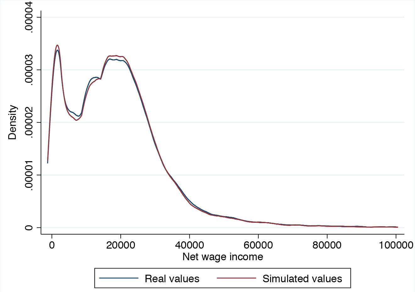
Figure 1

Distributions of the realized and the simulated values for net wage income.
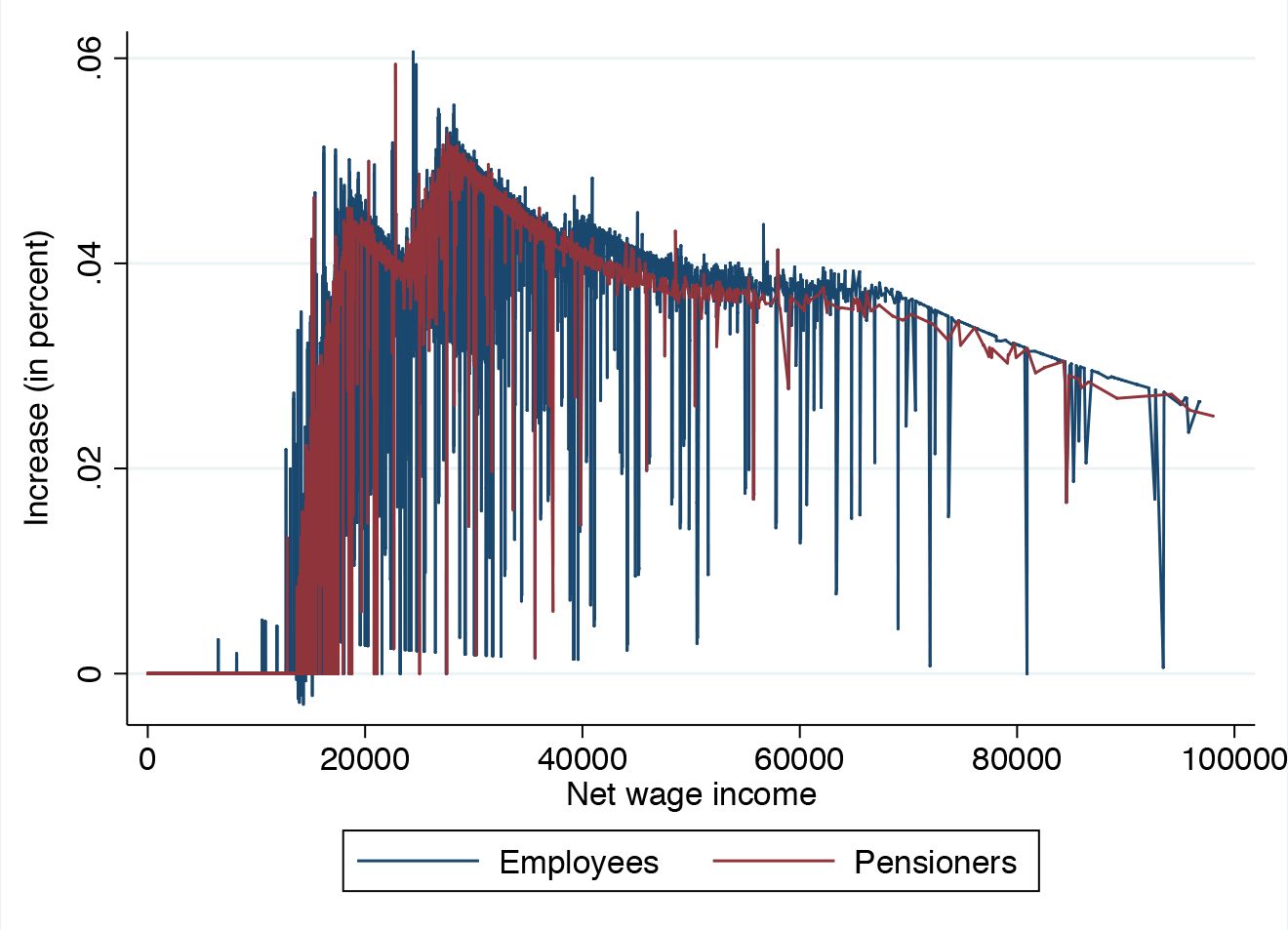
Figure 2

Annual net income increase of the 2016 tax reform.
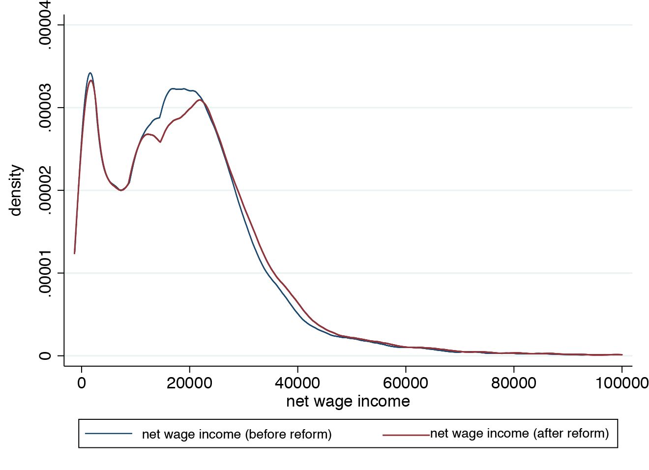
Figure 3

Distribution of net wage income before and after the 2016 tax reform.
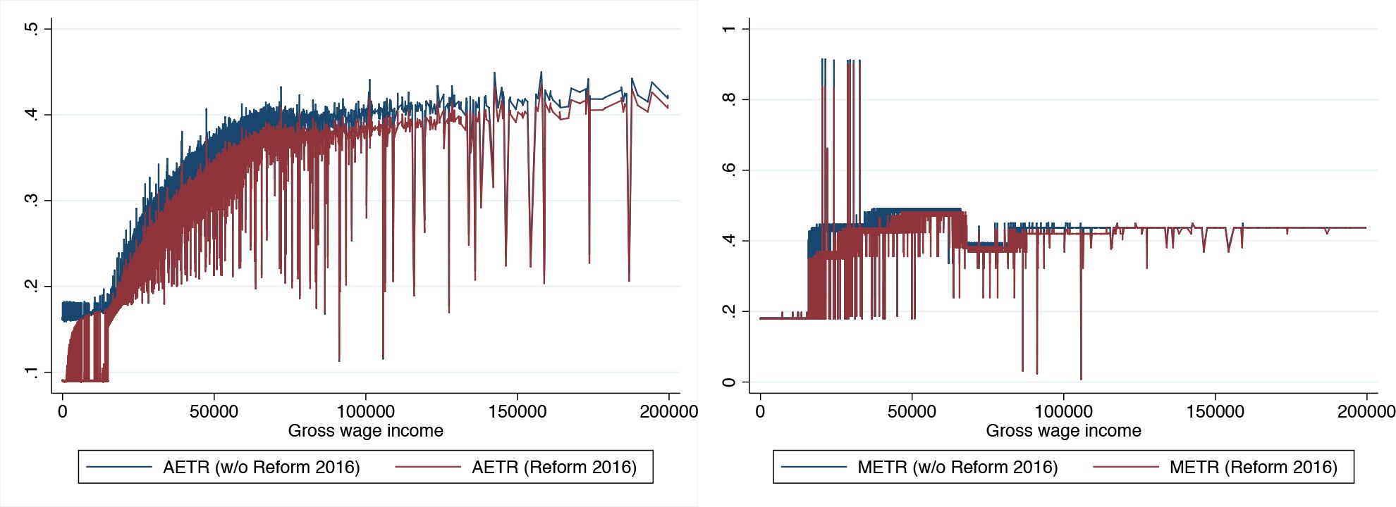
Figure 4

2016 tax reform – Incentives on the extensive margin (AETR) and intensive margin (METR).
Figure 5

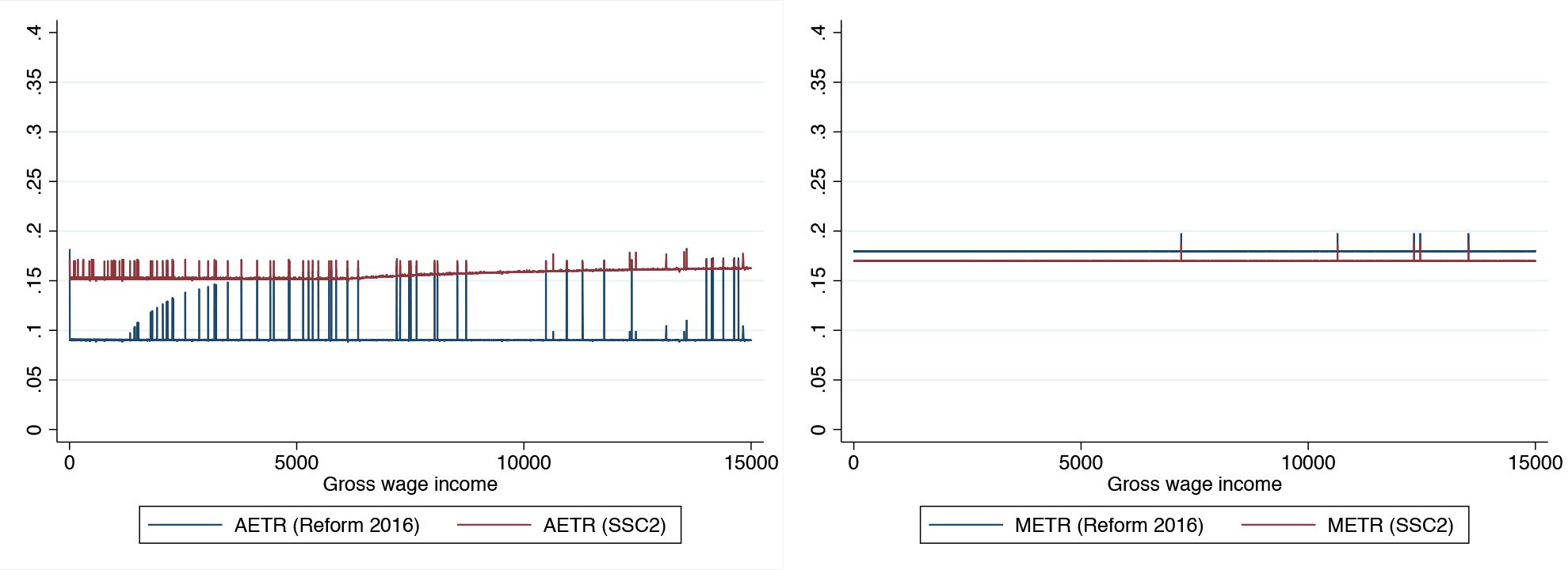
Policy options – Incentives for low wage incomes on the extensive (AETR) and intensive margin (METR).
Figure 6
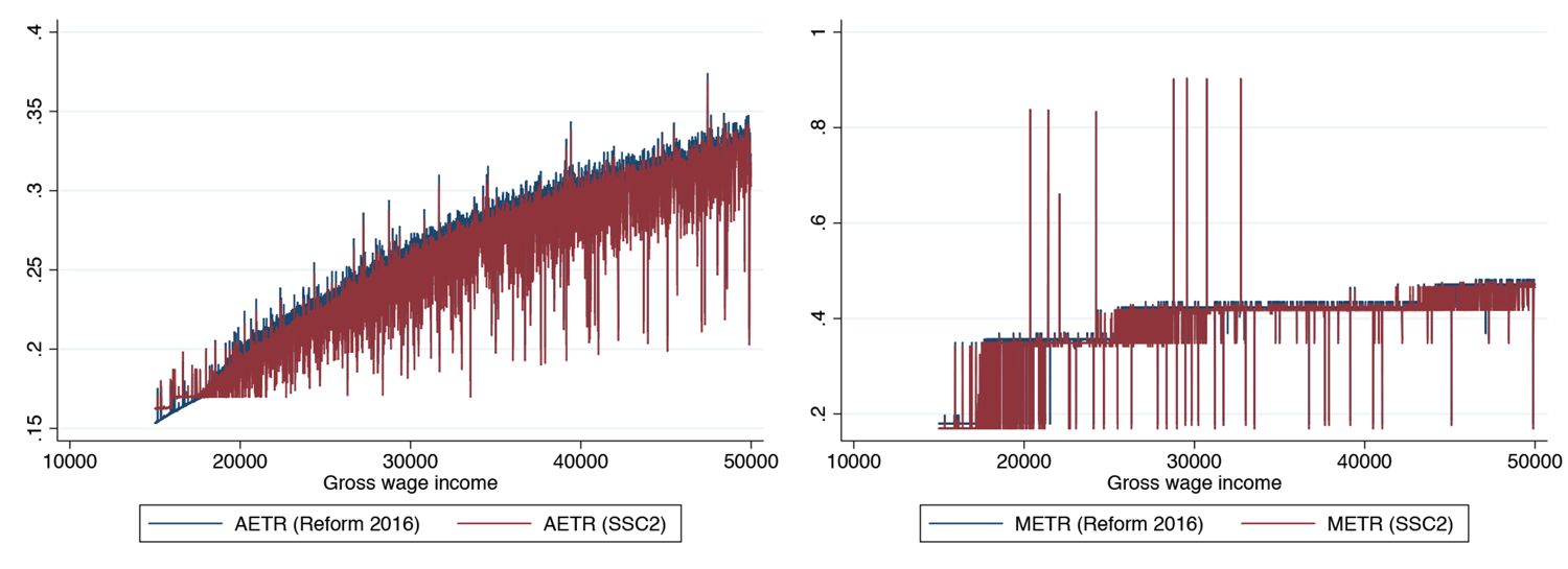
Policy options – Incentives for middle wage incomes on the extensive (AETR) and intensive margin (METR).
Figure A1

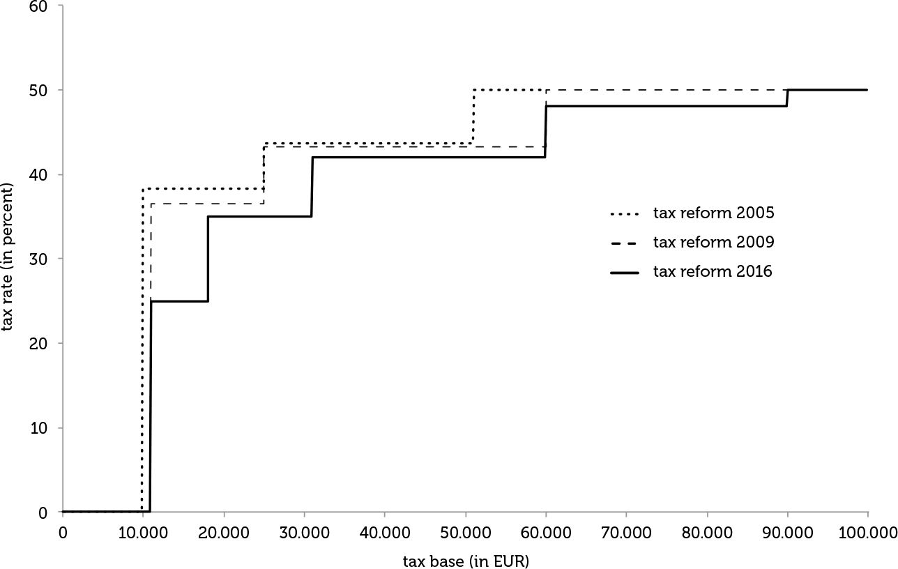
Tax rates in different tax reforms.
Tables
Table 1
The tax system in 2015.
| (a) Recurrent wage income tax rates. | |
|---|---|
| Tax base(EUR) | Tax rate |
| 0 – 11,000 | 0% |
| 11,000 – 25,000 | 36.5% |
| 25,000 – 60,000 | 42.21% |
| > 60,000 | 50% |
| (b) Tax rates for special payments. | |
| Tax base(EUR) | Tax rate |
| 0 – 620 | 0% |
| 620 – 25,000 | 6% |
| 25,000 – 50,000 | 27% |
| 50,000 – 83,333 | 35.75% |
| > 83,333 | 50% |
-
Source: Schratzenstaller (2009).
Table 2
Tax rates for recurrent wage in 2016.
| Tax base (EUR) | Tax rate |
|---|---|
| 0 – 11,000 | 0% |
| 11,000 – 18,000 | 0% |
| 18,000 – 31,000 | 35% |
| 31,000 – 60,000 | 42% |
| 60,000 – 90,000 | 48% |
| 90,000 – 1,000,000 | 50% |
| > 1,000,000 | 55% |
Table 3
Lump-sum allowances and tax credits.
| Old system | New system | |
|---|---|---|
| (EUR) | ||
| Tax credits: | ||
| employee tax credit | 54 | - |
| deductible amount for travel expenses | 291 | 400 |
| pensioner tax credit | 400 | 400 |
| Lump-sum allowances: | ||
| advertising expense lump-sum | 132 | 132 |
| extra charge lump-sum | 60 | 60 |
Table 4
Summary statistics (annual data).
| Variable | Mean | Std. Dev. | Obs. |
|---|---|---|---|
| (EUR) | |||
| Gross wage | 26,512.47 | 28,273.13 | 65,535 |
| Special payments (paragraph 67 (1–2) of the ESt)a | 3,437–61 | 3,284.93 | 65,535 |
| Social security and other contributions | 3,411.15 | 3,415.68 | 65,535 |
| Other wage income (paragraph 67 (3–8) of the ESt)b | 375.38 | 4,722.25 | 65,535 |
| Tax base | 18,982.57 | 21,216.19 | 65,535 |
| Total wage tax | 4,036.57 | 9034.34 | 65,535 |
-
a
The income tax law (“Einkommensteuergesetz 1988”, short ESt).
-
b
E.g. severance indemnities, dismissal wages etc.
Table 5
The simulation model.
| Gross wage income | |
|---|---|
| Recurrent wage income | special payments (13. and 14. payment) |
| + additional wage (except 13. and 14.) | |
| - social security contributions on recurrent income (see Table A.1) | |
| - lump-sum commuter allowance | - social security contributions on special payments |
| - other job-related allowances | |
| - non-job-related allowances | |
| = taxable recurrent income (tax base) | = taxable special payments (tax base) |
| - income tax (see Table 2) | - income tax |
| + tax credits | on special payments (see Table 1b) |
| = net wage income (recurrent wage income) | = net wage income (special payments) |
Table 6
Comparison of annual gross wage incomes: wage tax statistics 2014 and EU-SILC 2015.
| Percentile | Wage tax | EU-SILC | Difference |
|---|---|---|---|
| (EUR) | |||
| 10 | 4,463 | 2,860 | −35.9% |
| 20 | 10,743 | 8,061 | −25.0% |
| 30 | 16,943 | 14,938 | −11.8% |
| 40 | 22,420 | 20,774 | −7.3% |
| 50 | 27,714 | 26,612 | −4.0% |
| 60 | 32,704 | 31,903 | −2.4% |
| 70 | 38,367 | 38,265 | −0.3% |
| 80 | 46,483 | 45,809 | −1.4% |
| 90 | 61,317 | 59,943 | −2.2% |
| mean | 32,208 | 30,858 | −4.2% |
-
Source: Statistik Austria (2016)
Table 7
Monthly ceilings for social security contributions, 2016.
| Old system | New system | |
|---|---|---|
| (EUR) | ||
| Social security income cap | 4,750 | 4,860 |
| Social security income threshold | 416 | 416 |
Table 8
Summary statistics – simulated values (annual).
| Variable | Mean | Std. Dev. | N |
|---|---|---|---|
| (EUR) | |||
| Wage tax | 4,036.6 | 9,034.3 | 65,535 |
| Wag tax (sim) | 4,025.2 | 9,233.0 | 65,535 |
| Net wage income | 19,064.8 | 17,442.6 | 65,535 |
| Net wage income (sim) | 18,928.1 | 17,249.5 | 65,535 |
Table 9
Correlation realized values and simulated values.
| Wage tax | Net income | |
|---|---|---|
| Apprentices | 0.8508 | 0.9969 |
| Blue-collar workers | 0.9742 | 0.9979 |
| White-collar workers | 0.9931 | 0.9976 |
| Civil servants | 0.9905 | 0.9961 |
| Public-contract staff | 0.9853 | 0.9956 |
| Civil-servant pensioners | 0.9918 | 0.9972 |
| Pensioners | 0.9897 | 0.9971 |
| Individuals with care allowance | 1.0000 | 1.0000 |
| Other individuals | 0.9873 | 0.9975 |
| Total | 0.9922 | 0.9977 |
Table 10
Inequality measures.
| Inequality measure | Net income | Simulated net income |
|---|---|---|
| Gini coefficient | 0.40911 | 0.40706 |
| Theil index (GE(a), a = 1) | 0.31261 | 0.31107 |
| Atkinson inequality measures (eps = 1) | 0.35335 | 0.35734 |
Table 11
Changes in tax and social security revenues in 2016.
| Old system | New system | |
|---|---|---|
| (MEUR) | ||
| Total wage tax revenues | 27,644 | 23,451 |
| Net tax revenues | −4,193 | |
| Social security contributions | 23,912 | 24,039 |
| Net social security contributions | 127 | |
Table 12
Average annual net income by social groups.
| Old system | New system (EUR) |
Difference | ||
|---|---|---|---|---|
| Women | 14,504 | 14,920 | 416 | (2.87%) |
| Men | 24,107 | 24,942 | 836 | (3–47%) |
| Pensioners | 16,346 | 16,835 | 490 | (2.99%) |
| Employees | 20,673 | 21,362 | 689 | (3.33%) |
| Female employees | 16,511 | 17,021 | 510 | (3.09%) |
| Male employees | 24,363 | 25,211 | 848 | (3.48%) |
| Total | 19,179 | 19,799 | 620 | (3.23%) |
Table 13
Average annual net income by social status.
| Old system | New system (EUR) |
Difference | ||
|---|---|---|---|---|
| Apprentices | 7,255 | 7,627 | 372 | (5.12%) |
| Blue-collar workers | 14,616 | 15,075 | 459 | (3.14%) |
| White-collar workers | 25,112 | 25,940 | 828 | (3.30%) |
| Civil servant | 35,732 | 37,124 | 1,393 | (3.90%) |
| Public contract staff | 23,444 | 24,266 | 823 | (3.51%) |
| Civil servant pensioner | 29,850 | 31,058 | 1,208 | (4.05%) |
| Pensioner | 15,285 | 15,709 | 424 | (2.77%) |
| Other individuals | 8,927 | 9,145 | 218 | (2.45%) |
| Total | 19,179 | 19,799 | 620 | (3.23%) |
Table 14
Average annual net income by age.
| Old system | New system (EUR) |
Difference | ||
|---|---|---|---|---|
| 16 to 25 years | 10,054 | 10,351 | 297 | (2.96%) |
| 26 to 35 years | 18,260 | 18,884 | 624 | (3.42%) |
| 36 to 45 years | 22,306 | 23,056 | 749 | (3.36%) |
| 46 to 55 years | 25,133 | 25,972 | 838 | (3.34%) |
| 56 to 65 years | 22,313 | 23,005 | 692 | (3.10%) |
| 66+ years | 16,682 | 17,197 | 515 | (3.09%) |
| Total | 19,179 | 19,799 | 620 | (3.23%) |
Table 15
Inequality measures for 2016.
| Inequality measures | Old system | New system |
|---|---|---|
| Gini coefficient | 0.40606 | 0.41005 |
| Theil index (GE(a), a = 1) | 0.30688 | 0.31050 |
| Atkinson inequality measures (ε = 1) | 0.45917 | 0.46408 |
Table 16
Annual net wage income by deciles.
| Old system | New system (EUR) |
Difference | ||
|---|---|---|---|---|
| 1st decile | 735 | 735 | 0 | (0.00%) |
| 2nd decile | 3,905 | 3,912 | 7 | (0.18%) |
| 3rd decile | 8,704 | 8,730 | 26 | (0.30%) |
| 4th decile | 12,684 | 12,710 | 26 | (0.20%) |
| 5th decile | 16,081 | 16,468 | 387 | (2.40%) |
| 6th decile | 19,177 | 19,942 | 765 | (3.99%) |
| 7th decile | 22,303 | 23,185 | 882 | (3.95%) |
| 8th decile | 25,841 | 26,902 | 1,061 | (4.11%) |
| 9th decile | 30,954 | 32,337 | 1,383 | (4.47%) |
| 10th decile | 51,400 | 53,066 | 1,667 | (3.24%) |
Table 17
Theil decomposition by tax status (taxpayer or not).
| Old system | New system | |
|---|---|---|
| Total | 0.3069 | 0.3105 |
| Within | 0.1398 | 0.1377 |
| Between | 0.1671 | 0.1728 |
Table 18
Theil decomposition by social status, working time, age groups and gender.
| (a) by social status | (b) by working time | |||
|---|---|---|---|---|
| Old system | New system | Old system | New system | |
| Total | 0.3069 | 0.3105 | 0.3069 | 0.3105 |
| Within | 0.2521 | 0.2551 | 0.2526 | 0.2548 |
| Between | 0.0547 | 0.0554 | 0.0543 | 0.0557 |
| (c) by age groups | (d) by gender | |||
| Old system | New system | Old system | New system | |
| Total | 0.3069 | 0.3105 | 0.3069 | 0.3105 |
| Within | 0.2718 | 0.2752 | 0.2872 | 0.2903 |
| Between | 0.0351 | 0.0353 | 0.0197 | 0.0202 |
Table 19
Costs of the policy proposals.
| Old system | New system | Proposals | ||
|---|---|---|---|---|
| SSC1 | SSC2 | |||
| (MEUR) | ||||
| Wage tax revenue | 23,451 | 24,006 | 23,830 | |
| SSC revenue | 24,039 | 22,389 | 22,883 | |
| Additional wage tax revenue | 556 | 379 | ||
| Loss in SSC | −1,649 | −1,155 | ||
| Total costs | −370 | −1,094 | −776 | |
Table 20
Impact of policy options on wage income deciles.
| Old system | New system 400 EUR NIT | Proposals | |||||
|---|---|---|---|---|---|---|---|
| SSC1 | SSC2 | ||||||
| (EUR) | |||||||
| 1st decile | 780 | +16 | (2.07%) | +7 | (0.92%) | +8 | (0.97%) |
| 2nd decile | 3,980 | +196 | (4.92%) | +51 | (1.28%) | +52 | (1.32%) |
| 3rd dec1le | 8,771 | +243 | (2.78%) | +122 | (1.40%) | +126 | (1.43%) |
| 4th dec1le | 12,715 | +164 | (1.29%) | +162 | (1.27%) | +167 | (1.31%) |
| 5th dec1le | 16,081 | +391 | (2.43%) | +529 | (3.29%) | +535 | (3.33%) |
| 6th dec1le | 19,177 | +765 | (3.99%) | +925 | (4.82%) | +932 | (4.86%) |
| 7th dec1le | 22,303 | +882 | (3.95%) | +1,066 | (4.78%) | +1,075 | (4.82%) |
| 8th dec1le | 25,841 | +1,061 | (4.11%) | +1,287 | (4.98%) | +1,297 | (5.02%) |
| 9th dec1le | 30,954 | +1,383 | (4.47%) | +1,647 | (5.32%) | +1,590 | (5.14%) |
| 10th dec1le | 51,400 | +1,668 | (3.24%) | +2,075 | (4.04%) | +1,672 | (3.25%) |
Table 21
Inequalitymeasures and Theil decomposition of policy options.
| New system 110 EUR NIT | New System 400 EUR NIT | Proposals | ||
|---|---|---|---|---|
| SSC1 | SSC2 | |||
| Gini coefficient | 0.405 | 0.406 | 0.408 | 0.407 |
| Theil Total | 0.305 | 0.306 | 0.308 | 0.307 |
| Theil Within | 0.140 | 0.137 | 0.137 | 0.136 |
| Theil Between | 0.166 | 0.168 | 0.171 | 0.171 |
Table A1
Social security contributions.
| HI | PI | UI | add. taxes | Total | |
|---|---|---|---|---|---|
| 2015 | |||||
| other individuals | 3.82% | 10.25% | 3.00% | 1.00% | 18.07% |
| apprentices | 3.95% | 10.25% | 3.00% | - | 17.20% |
| blue-collar workers | 3.95% | 10.25% | 3.00% | 1.00% | 18.20% |
| white-collar workers | 3.82% | 10.25% | 3.00% | 1.00% | 18.07% |
| civil servant | 4.10% | 11.80% | 3.00% | 1.00% | 19.90% |
| public contract staff | 3.82% | 10.25% | 3.00% | 1.00% | 18.07% |
| civil servant pensioner | 5.10% | 10.25% | - | - | 15.35% |
| pensioner | 4.90% | 10.25% | - | - | 15.15% |
| individual with care allowance | 4.90% | 10.25% | - | - | 15.15% |
| 2016 | |||||
| other individuals | 3.87% | 10.25% | 3.00% | 1.00% | 18.12% |
| apprentices | 1.67% | 10.25% | 1.20% | - | 13.12% |
| blue-collar workers | 3.87% | 10.25% | 3.00% | 1.00% | 18.12% |
| white-collar workers | 3.87% | 10.25% | 3.00% | 1.00% | 18.12% |
| civil servant | 4.10% | 11.75% | 3.00% | 1.00% | 19.85% |
| public contract saff | 3.87% | 10.25% | 3.00% | 1.00% | 18.12% |
| civil servant pensioner | 5.10% | 10.25% | - | - | 15.35% |
| pensioner | 5.10% | 10.25% | - | - | 15.35% |
| individual with care allowance | 5.10% | 10.25% | - | - | 15.35% |
Table A2
Independent 2-group Mann-Whitney U Test.
| W | p-value |
|---|---|
| 2,152,840,096 | 0.4286 |
-
Note: Alternative hypothesis – true location shift is not equal to 0.
Download links
A two-part list of links to download the article, or parts of the article, in various formats.