MILC: A microsimulation model of the natural history of lung cancer
- Brown University School of Public Health, United States
Abstract
The Microsimulation Lung Cancer (MILC) model was developed to simulate individual trajectories and predict outcomes of lung cancer for populations. The model describes the natural history of lung cancer from a disease-free state to death. Predictions of individual trajectories depend on a set of covariates including age, sex, and smoking behaviors. The module presented here is designed as part of a comprehensive decision-making toolkit for evaluating lung cancer prevention, screening and treatment policies. The MILC package implements the model in the open-source statistical software R. This paper introduces the main components, simulation algorithm, and specifics of the MILC model, validates it by reproducing observed lung cancer incidence trends in the US population, and uses it to make plausible predictions for 50-year-old men and women with a range of smoking histories.
1. Introduction
Micro-Simulation Models (MSMs) are predictive models designed to describe complex processes and simulate unit level data (Orcutt, 1957). Predicted trends about the quantities of interest, resulting from aggregation of a large number of microsimulations, are intended to guide policy decisions. In medical decision making MSMs usually describe the natural history of a disease, often in conjunction with the effect of some intervention, such as screening, treatment, etc. (Kopec, Edwards, Manuel, & Rutter, 2012). To this end they employ mathematical equations with stochastic assumptions to describe both observed and latent characteristics of the underlying process (Rutter, Zaslavsky, & Feuer, 2011).
MSMs are useful because they provide a handy way to simulate intricate phenomena involving dynamic systems for which observed data are either hard or even unethical to collect (for instance, exposing the subjects to unnecessary risks) or not available (for example, latent characteristics). They also constitute a practical tool for combining information from various sources, including observational studies, clinical trials, expert opinions, etc., and simulating large pseudo-samples. Due to the great flexibility they provide to researchers, MSMs have proven so far one of the best ways to model the progression of chronic diseases (Oderkirk, Sassi, & Cecchini, 2012). The focus on the individual rather than the average patient can also prove them a very useful tool for assisting improvement of individualized patient care. Therefore microsimulation has risen to prominence as a promising tool for making projections about the impact of interventions (such as screening) when applied to population cohorts, and thus informing health policies and improving medical decision making (Kopec et al., 2012). For example MSMs are often used in Comparative Effectiveness Research (CER) studies, aimed at evaluating public health policies and their effect on health status of target populations Zucchelli, Jones, & N., 2012.
The development of an MSM is a challenging undertaking. Due to their complexity (combination of several stochastic and deterministic models, a usually large number of parameters, description of latent characteristics, etc.), model calibration requires advanced statistical techniques, and a huge number, usually of an order of magnitude of 12 or more, of microsimulations. The same holds for an extensive validation of the model, let alone a sensitivity analysis, hence it is self evident that the development of an MSM is a computationally highly intensive problem that necessitates special resources for implementing high performance computing techniques. Furthermore, the complexity of an MSM along with the fact that it often tries to describe latent phenomena lead to identifiability problems. The degree of accuracy and the validity of an MSM highly depend on the available information and data for building and calibrating the model. In addition, MSMs are subject to several sources of uncertainty, the combination and expression of which on the final outcomes is a problem not satisfactorily addressed yet (Li & O’Donoghue, 2013; Rutter et al., 2011).
Several MSMs have been developed in order to predict lung cancer related outcomes. Some of the most comprehensive ones are part of the research conducted by the Cancer Intervention and Surveillance Modeling Network (CISNET) of the National Cancer Institute (NCI).1 Examples of other MSMs for lung cancer can also be found in the literature (Bongers et al., 2016, 2013; Flanagan et al., 2015; Goldwasser, 2009). All these models, as part of interdisciplinary work, have been proven extremely useful, especially for evaluating intervention strategies and informing public health decisions, with numerous applications. Depending on the specific purpose to fulfill, each of these MSMs focuses on particular aspects of the natural history of lung cancer, exhibiting large variation from the structure (methods used to describe each component, etc.) and required input data, to the predicted outcomes.
Despite the evident usefulness, and unquestionable value and contribution in the field of lung cancer research, MSMs for lung cancer suffer from some limitations. Until today, at least to our knowledge, there is no publicly available source code for running these models. In addition, the high level of complexity, and the lack, in many cases, of sufficient details about their structure, render these models “black boxes’’, hard to understand and evaluate, and impossible to reproduce (Kopec et al., 2010; Rutter et al., 2011). The implementation, and reporting practices for MSMs require a lot of discussion, and some standardization, in order to facilitate evaluation and enhance comprehensiveness.
The Microsimulation Lung Cancer (MILC) model (Chrysanthopoulou, 2013), is a new, dynamic, continuous time microsimulation model that simulates individual trajectories focusing on lung-cancer related outcomes. In its current version, the model comprises a module describing the natural history of lung cancer in the absence of any screening or treatment components, and incorporates several best current practices for modeling lung cancer states. The model simulates the course of lung cancer from the disease-free state to the local, regional, and distant disease states and eventually to death either from lung cancer or some other cause. Prediction of individual trajectories involves incorporation of unit-level baseline information about three important factors, namely age, sex, and smoking, including current smoking status, start and quit smoking ages, and average number of cigarettes smoked per day when relevant.
One of the main objectives of creating MILC was to use the model as a tool for studying the statistical properties of, and suggesting appropriate statistical methods for the development of MSMs with analogous characteristics. Furthermore we wanted to create a streamlined, yet valid MSM for lung cancer, and make it publicly available to potential end users in the field of lung cancer research. The MILC package (Chrysanthopoulou, 2014) includes the required source code and data for implementing this model in the open-source statistical software R, and is available on the Comprehensive R Archive Network (CRAN) repository.
This article introduces the MILC model and describes its main components, simulation algorithm, and specifications. We also present two examples of how the MILC model can be used in practice. In the first example we validate the model against observed lung cancer incidence rates in the US population, while in the second we use the MILC model to predict individual risks for smokers based on sex and smoking intensity. Finally we discuss the main differences between our model and other MSMs used in lung cancer research, and outline future work to develop the MILC model into a comprehensive tool for assisting decision making for lung cancer.
2. Methods
2.1 Model components
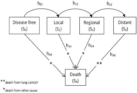
The MILC model defines five distinct states in the natural history of lung cancer. Starting from the disease-free state (S0) it is possible for an individual to have transition to the local (S1), regional (S2), and distant (S3) disease state, and eventually to the absorbing state of death (S4) either from lung cancer or from some other cause. States S1-S3 are sometimes called tunnel states because of their special arrangement, namely they can only be visited in this particular fixed order (Sonnenberg & Beck, 1993). The Markov state diagram in Figure 1 depicts the five distinct MILC model states, and the underlying transition rules.

Markov state diagram of the MILC model.
The onset of the first malignant cell signifies the beginning of the local disease state (S1). The tumor in that state is limited to the place where it started, with no sign of spread elsewhere in the body. The first malignant cell can proliferate up to the point of nearby lymph nodes, tissues, or organs involvement thus transitioning to the regional disease state (S2). The tumor may further progress to the distant state (S3), namely metastasize to distant parts of the body, and eventually cause death (S4), unless death from some other cause precedes. Within the three tunnel states tumor can range from Stage 0 to Stage IV, depending on the size and spread (National Cancer Institute, 2017a).
The MILC model makes some important assumptions. First of all it assumes that the transition to subsequent states depends only on the present state (Markov property). Furthermore the disease progression is irreversible, namely once the first malignant cell occurs lung cancer will either remain to the local or transition to subsequent states, depending on the total time of the follow-up period and a number of risk factors. Finally a death can be attributed to lung cancer if and only if it occurs after transition to the distant state.
2.1.1 Onset of the first malignant cell
We model the onset of the first malignant cell using the exact solutions for the expression of the hazard rates and the survival probabilities of the biological two-stage clonal expansion (TSCE) model suggested by Moolgavkar and Luebeck (1990). According to this model the hazard function for the development of the first malignant cell (Heidenreich, Luebeck, & Moolgavkar, 1997) can be expressed as:
with γ = α − β − µ, and
Studies (Hazelton, Clements, & Moolgavkar, 2005; Hazelton, Luebeck, Heidenreich, & Moolgavkar, 2001) have shown that power laws are good approximations to the effect of smoking on the onset of the first malignant cell. If q(t) denotes the smoking intensity at age t, expressed as average number of cigarettes smoked per day, then:
and
where αns and γns are the respective coefficients for non-smokers. To account for sex and smoking history differences, we assume different hazards (as functions of age t) for each combination of sex (male/female), and smoking status (never/former/current smoker) categories.
For each individual the time period from birth (t = 0) to the onset of the first malignant cell can be split into intervals within which the hazard rate is constant and depends on the person’s smoking status. The hazard for never smokers is constant throughout their entire life and of course independent of smoking. Smokers have two different hazards, one before (the same with non-smokers), and one after (depending on the smoking intensity) they start smoking. In its current version MILC also assumes that former smokers had only two changes in their smoking behavior, namely one when they started and one when they quit smoking. However the model is flexible and can accommodate multiple changes of smoking behavior in a person’s lifetime.2
2.1.2 Tumor growth
The Gompertz distribution is more flexible than the exponential, and therefore provides a better approximation of tumor growth for most cancer types (Detterbeck & Gibson, 2008). The Gompertz distribution models proliferation of tumor cells as a modified exponential process in which successive doubling times occur at increasingly longer time intervals (Laird, 1964). This enables us to capture the reality of shorter pre-clinical periods with longer survival after diagnosis.
We define V(t) to be the tumor volume when a person reaches age t (in years). The MILC model assumes a Gompertzian tumor growth (Laird, 1964), according which:
where V0 represents the initial tumor volume (namely the volume of the first malignant cell), while m is the scale, and s is the shape parameter of the Gompertz probability density function.
We further assume a spherical tumor growth (Gallaher, Babu, Plevritis, & Anderson, 2014), thus making the tumor size a function of its diameter d(t) at age t, namely:
In the literature (Detterbeck & Gibson, 2008; Geddes, 1979; McMahon, 2005) we find that the minimum tumor diameter (one cancerous cell) is d0 = 0.01µm, and the maximum possible diameter (tumor that causes death) is dmax = 13cm. To simplify model parameterization we assume the same Gompertz distribution for all tumors irrespective of their histological type and stage.
2.1.3 Disease progression
Disease progression of an existing lung cancer can occur via nodal involvement and distant metastases (McMahon, 2005). Current MSMs for lung cancer (Goldwasser, 2009; McMahon, 2005) in their disease progression parts adopt methods developed to describe the progress of breast cancer (Garg, Rao, & Redmond, 1970; Koscielny, Tubiana, & Valleron, 1985; Plevritis, Salzman, Sigal, & Glynn, 2007; Thames, Buchholz, & Smith, 1999). Given a Gompertzian tumor growth, the log-normal distribution can adequately describe the distribution of tumor volumes at specific time points, starting from the local state, that is the onset of the first malignant cell (Koscielny et al., 1984, 1985; Spratt & Spratt, 1964; Steel, 1977).
We define three different log-normal distributions to simulate the tumor volume at the transition to regional (Vreg), and distant (Vdist) disease states, as well as the tumor at diagnosis (Vdiag). Given the simulated tumor volume, and growth rate, and assuming a spherical growth, the model calculates the age at which the tumor has reached a specific size, and hence the age at the transition to each of the respective three MILC states.
2.1.4 Survival
Because smoking is an important risk factor for dying not only from lung cancer (National Cancer Institute, 2017b), we follow a competing risks approach to simulate mortality, distinguishing between death from lung cancer or other causes. We estimate the probability of death from lung cancer in the presence of other causes of death, using the Cumulative Incidence Function (CIF) non-parametric technique (Klein & Moeschberger, 2003). We derive estimates using information from both the National Health Interview Survey (NHIS, 2006) and Surveillance, Epidemiology and End Results (SEER, 2006) data.
We employ the inverse transform approach to simulate both age and cause of death (lung cancer or other) based on CIF estimates. The MILC simulations depend on the strong assumption that the observed death patterns and smoking behaviors do not change dramatically over time, hence they are also relevant to the prediction period we are interested in. Furthermore, given the data used, the model currently represents survival patterns observed in the US population. Depending on the available information, the MILC model can be also calibrated and used to simulate other (sub-)populations.
2.2 Model specifics
2.2.1 Structure and parameterization
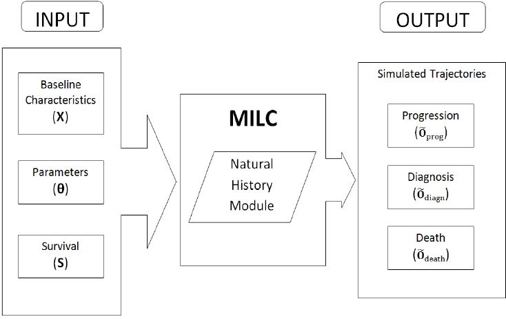
Table 1 summarizes the parameterization of the MILC model. Figure 2 depicts how the model functions, namely the required input and the anticipated output for each simulated individual trajectory. In particular, to predict one trajectory, we “feed” the model with three sets of input: (i) Baseline characteristics X (age, sex, smoking habits) of the individual. Smoking includes status (never, former, or current smoker), as well as start and quit smoking ages, and smoking intensity (average number of cigarettes smoked per day), where relevant. (ii) Values for the model parameters θ. These values can be either ad-hoc estimates or the result of some calibration procedure. (iii) Cumulative incidence function estimates S for lung cancer and other cause survival.
Possible MILC outputs (predictions) can be classified into three broad categories, namely those regarding the disease progression (Õprog), diagnosis (Õdiagn), and death (Õdeath). Disease progression output (Õprog = {Tmal, Treg, Tdist}), comprises prediction of the ages at the beginning of the local, regional, and distant tumor states respectively. In the MILC model diagnosis signifies the time when lung cancer is confirmed and assessed for its size and stage. Diagnosis output (Õdiagn = {Tdiagn, ddiagn, stage}) includes predicted age, tumor size, and tumor stage at diagnosis. Finally, death output (Õdeath = {Tdeath, cause}) has information about the age and cause of death, if the model predicts that the individual dies before the end of the follow-up period. Otherwise it provides the age at the end of the prediction period, if the person is still alive by then.
MILC model parameterization.
| Model components |
|---|
| Initiation of the local stage: Two-Stage Clonal Expansion (TSCE) carcinogenesis model |
| Risk for the onset of the first malignant cell: |
| where
γ = α − β − µ and X: total number of normal stem cells ν: normal cell initiation rate α: division rate of initiated cells β: apoptosis rate of initiated cells µ: malignant conversion rate of initiated cells |
| Effect of smoking on α and γ parameters: <disp-formula id="equu1"> </disp-formula> |
| where q(t): average number of cigarettes smoked per day at age t (αs, γs) and (αns, γns): parameters for smokers and non-smokers respectively. |
| Tumor growth: Gompertz function <disp-formula id="equu2"> </disp-formula> |
| where V(t): tumor volume at age t V0: minimum tumor volume (one malignant cell) |
| Assuming spherical tumor growth:
<disp-formula id="equu3">
</disp-formula>
d(t): diameter at age t d0 = 0.01mm, diameter of one malignant cell dmax = 13cm, maximum tumor diameter |
| Disease progression: Transition to regional and distant stages and tumor diagnosis |
| Tumor volume at: — the beginning of the regional stage: Vreg ~ log-normal (µreg, sdreg) — the beginning of the distant stage: Vdist ~ log-normal (µdist, sddist) — diagnosis: Vdiagn ~ log-normal(µdiagn, sddiagn) |
| where <disp-formula id="equu4"> </disp-formula> |

Structure of the MILC model.
2.2.2 Calibration
Specifying the parameter values of an MSM requires extensive calibration with results heavily depending on the quality of the available data. The microdata used and the calibration targets set are key components of the calibration procedure. Microdata is essentially individual-level information for a sample of subjects representative of the target population in the study and is used as input to the model for simulating individual trajectories. Calibration targets are quantities of interest (usually summary statistics from the target population) that the MSM should accurately predict.
The high level of complexity usually renders impossible the determination of closed-form expressions of the outcomes as functions of the model parameters. This along with the fact that an MSM usually involves description of latent characteristics, as is the case with the MILC model, dictates the use of calibration procedures for the specification of sets of plausible values for the model parameters. Detailed calibration of an MSM is a computationally intensive and time consuming process. For the examples presented in this paper we have used the MILC model after calibrating four parameters, and setting ad-hoc estimates or fixed values from the literature for the others as indicated in Table 2.
The microdata used for this calibration, included individual-level information randomly extracted from the 1980 US population. The four parameters that we chose to calibrate represent several aspects in the natural history of lung cancer; one is related to the tumor growth (m), and the others to the disease progression component of the model (μregj, μdist, and μdiagn). We used fixed values for all the other MILC parameters, based on literature review about the natural history of lung cancer (Table 2). For parameters related to the onset of the first malignant cell we retrieved values from Hazelton et al. (2005), while values for the tumor growth component were found in Koscielny et al. (1985).
We implemented the Bayesian calibration method, suggested by Rutter, Miglioretti, and Savarino (2009), to calibrate the MILC model on lung-cancer incidence trends observed in the 2006 US population of males. The method involves a large number of Gibbs sampler iterations with embedded approximate Metropolis-Hastings steps for drawing values from the joint posterior distribution, assuming that lung cancer incidence rates approximately follow a Poisson distribution. The result from this calibration method is a set of random draws from the approximate joint posterior h(θ | Y ) of the parameter vector θ. Table 2 presents medians and interquartile ranges for the four calibrated MILC parameters (m, µreg,µdist, and µdiagn).
Details on the Bayesian calibration procedure are provided in another paper in preparation (Chrysan-thopoulou, 2017). This paper discusses results from a comprehensive comparative analysis of two of the most broadly used calibration methods for MSMs, the aforementioned Bayesian method, and another Empirical technique which employs the Latin Hypercube Sampling design for an efficient search of the multidimensional parameter space.
2.2.3 Validation
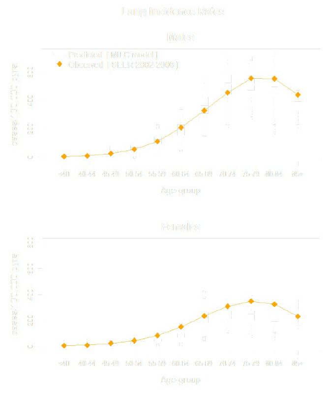
We validated the model predictions against lung cancer incidence trends observed in the US population. For this purpose we simulated individual-level characteristics (age, sex and smoking) for a pseudo-sample of size N=10,000 people, representative of the 1980 US population, combining information from the 1980 US census, and the 1980 Statistical Abstract of the US. We used the calibrated MILC model to simulate individual trajectories for people in the pseudo-sample, and predicted lung cancer incidence rates 26 years ahead. We compared the predicted rates (aggregated results) with age-group specific ones reported in the SEER 2002–2006 database (Figure 3). The MILC model can also be calibrated to other data, so as to simulate various (sub-)populations, and/or even reproduce other lung cancer related outcomes, such as mortality, age and tumor stage at diagnosis.
2.2.4 Functionality
The most typical use, and essentially the primary reason which has driven the development and implementation of MSMs in medical decision making, is the application of this model to a cohort of people for which individual-level information at baseline is available. Given this information, the model tries to accurately predict individual disease trajectories, and estimate outcomes of interest by aggregating relevant quantities from the predicted trajectories (Meza et al., 2014; Rutter & Savarino, 2010; Wolf-son, 2011). Those estimates can result in after a single or multiple runs of the model on the same cohort. Multiple repetitions are preferable because they can provide a better sense of the inherent uncertainty, and reveal interesting correlation structures of the underlying system components.
Values and calculations for the fixed and calibrated parameters of the MILC model.
| Parameter | Sex | Description | |
|---|---|---|---|
| Male | Female | ||
| Onset of the first malignant cella | |||
| All | |||
| X | IOe+7 | Total number of normal stem cells | |
| Non-Smokers | |||
| vns | 7.16e-8 | 1.07e-7 | Normal cell initiation rate |
| αns | 7.7 | 15.82 | Division rate of initiated cells |
| γns | 0.09 | 0.071 | |
| µns | vns | Malignant conversion rate of initiated cells | |
| βns | αns − µns γns | Apoptosis rate of initiated cells | |
| Smokers | |||
| νs | νns | 0.98xνns | Normal cell initiation rate |
| α1 | 0.6 | 0.5 | |
| α2 | 0.22 | 0.32 | |
| αs | αns×(I+α1 × [q(t)]α2) | Power law relationships between γ, α and | |
| γs | γns×(I+α1 × [q(t)]α2) | smoking intensity q(t) at age t | |
| µs | µns | Malignant conversion rate of initiated cells | |
| βs | αs − µs − γs | Apoptosis rate of initiated cells | |
| Tumor growthb | |||
| d0 | 0.01mm | Minimum tumor diameter (one tumor cell) | |
| dmax | 130mm | Maximum tumor diameter | |
| m | 3.4e-4 | Scale parameter of the Gompertz distribution | |
| [3.2e-4, 3.6e-4] | |||
| s | 31× m | Shape parameter of the Gompertz distribution | |
| Disease progression | |||
| µreg = sdreg | 2.16 [1.37, 3.06] | Mean and sd of the logNormal distribution for | |
| µdist = sddist | 5.62 [3.59, 8.02] | the tumor volume at the beginning of the regional, | |
| µdiagn = sddiagn | 2.65 [1.52, 3.94] | distant stage, and diagnosis | |
-
Notes: Values for the calibrated MILC parameters are presented as Q2 [Q1, Q3], where Q2 is the median, and Q1, Q3 are the 1st and 3rd quartiles respectively. The values and distributions of MILC parameters are the same for males and females, unless otherwise indicated.
-
Sources:
-
a
Ad hoc values from Hazelton et al. (2005).
-
b
Ad hoc values from Koscielny et al. (1985).
In this paper we also suggest another potential use of a well calibrated MSM. Given certain baseline characteristics, the model can be run multiple times on the same individual so as to produce a set of possible patient-specific trajectories. Summarizing information from these simulated trajectories can result in useful estimates about disease-related outcomes, and inform clinical decisions for the particular person. In another paper in preparation (Chrysanthopoulou, 2018) we emphasize the need for MSMs that can accurately predict individual-level outcomes, and help with improving individualized-patient care. In that paper we also discuss statistical methods for assessing the predictive accuracy of continuous time, dynamic MSMs, using MILC as a tool for the implementation and comprehensive comparison of those techniques.
We exemplify the functionality of our model by presenting results from two applications. The first example is related to model validation, namely MILC is used to predict lung cancer incidence rates for the US population, as described in Section 2.2.3. Comparison of these predictions with observed lung cancer incidence rates from the SEER database constitutes an external validation of the MILC model in the sense that the microdata for this procedure were different from the sample used for calibrating the model.
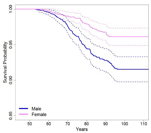
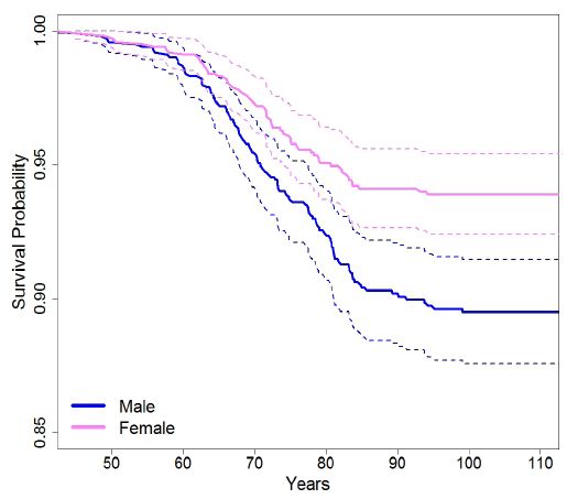
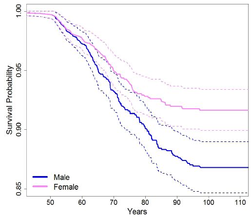
Furthermore we used MILC to estimate individual risk of developing lung cancer under different scenarios. To accomplish this we ran the model multiple times (n = 1000) on the same individual (fixed baseline characteristics), and simulated lifetime trajectories. We considered scenarios for smokers (males and females), who were 50 years old at baseline, and started smoking around the age of 20 years. We varied smoking intensity to an average of 10,30, or 50 cigarettes per day, in order to assess the effect of this important risk factor on the predicted lung cancer incidence. We summarized predicted event (lung cancer diagnosis) or censoring (if the person is not diagnosed with lung cancer before death) times with Kaplan-Meier curves.
2.2.5 Implementation in R
One of the main objectives of this research was to create an MSM for lung cancer fully developed in open source software, thus enhancing the transparency of the model. To this end Chrysanthopoulou (2014) built MILC, a new R-package that implements the MILC model in R, and is available on the CRAN repository. This package can be used to simulate individual trajectories, and predict lung-cancer related outcomes following the structure and assumptions of the MILC model.
Table A.1 outlines the algorithm for simulating one individual trajectory (one microsimulation). The computational cost for running in parallel 1,000,000 independent microsimulations (individual trajectories) was approximately 7.5 CPU-hours; with simulations distributed across 16 nodes (8-core Intel Xeon E5540 at 2.53 GHz with 24GB of memory) the total required time is 3.5 minutes.
3. Results
Figure 3 shows the results from the validation of the MILC model. The box plots summarize the distributions of the predicted lung cancer incidence rates by age-group for male and female current smokers. All observed rates fall within the resulting range of model-predicted values, thus suggesting an overall good performance of the Bayesian calibrated MILC model with respect to predicting lung cancer incidence trends in the particular US sub-population.

Predicted versus observed lung cancer incidence rates by age-group and sex.
We also used the calibrated MILC model to simulate lifetime trajectories for individuals given certain baseline characteristics (Section 2.2.4). We summarized predictions about the development of lung cancer with Kaplan-Meier curves. Figure 4, Figure 5, and Figure 6 compare predicted survival curves by sex and smoking intensity. According to model’s predictions, males have a greater risk of lung cancer than females. In addition, as expected, the risk of developing lung cancer increases with the average number of cigarettes smoked per day. Both these findings are consistent with current lung cancer research (Doll, 1998; American Cancer Society, 2017; IARC, 1986), thus indicating that the MILC model can provide plausible predictions.

Predicted individual risk of lung cancer for people, 50 years old, smoking on average 10 cigarettes per day, by sex.
4. Discussion
This paper introduces the MILC microsimulation model that describes the natural history of lung cancer, and predicts lung cancer related outcomes. The model simulates individual trajectories given age, sex and smoking, including smoking status (never, former, or current smoker), intensity (average number of cigarettes smoked per day), as well as start and quit smoking ages when relevant. Each simulated trajectory includes information regarding the age of transition to any of four distinct states in the course of lung cancer (that is, local, regional, distant, death), the age, tumor size and stage at diagnosis, and the cause of death (lung cancer, or other) where relevant. The MILC package (Chrysanthopoulou, 2014) implements the MILC model in R, and is available on the CRAN repository.
We outlined the model structure and parameterization, and described the simulation algorithm for predicting individual trajectories. We calibrated and validated the model against lung-cancer incidence rates observed in the US population. We further used the calibrated MILC model to predict lung cancer incidence risk for different subpopulations of smokers classified by sex and smoking intensity. The results showed an overall good fit of the MILC model to observed data, as well as plausible predictions with respect to the effects of sex and smoking on lung cancer incidence.

Predicted individual risk of lung cancer for people, 50 years old, smoking on average 30 cigarettes per day, by sex.

Predicted individual risk of lung cancer for people, 50 years old, smoking on average 50 cigarettes per day, by sex.
The CISNET lung cancer group has developed some of the most comprehensive, and broadly used microsimulation models, among the several predictive models for lung cancer in the literature. This group has currently six predictive models for lung cancer, among which four are microsimulation models. The SimSmoke model (Levy, Bauer, & Lee, 2006; Levy & Friend, 2002) and the Yale University model (Holford, Zhang, & Mckay, 1994; Holford, Zhang, Zheng, & McKay, 1996) are not microsimulation models, as they adopt the cohort-simulation representation of the underlying Markov process, rather than a Monte Carlo simulation.
Among the other four CISNET MSMs for lung cancer, the RICE-MDA model by Foy, Deng, Spitz, Gorlova, and Kimmel (2012) predicts lung-cancer mortality without any detail on disease progression, such as tumor growth, age, tumor type and stage at diagnosis, etc. The FHCRC model by Hazelton, Jeon, Meza, and Moolgavkar (2012) only comprises a natural history component, as the module we suggest in this article. However, unlike the MILC, the FHCRC model focuses on the effect of smoking on lung-cancer mortality without providing an explicit definition of the distinct disease states, or information on tumor diagnosis. The MISCAN-lung model by Habbema, van Oortmarssen, Lubbe, and van der Maas (1985), on the other hand, does not monitor tumor size in the simulation procedure. Finally, the key difference between the MILC and the Lung Cancer Policy Model (LCPM) by McMa-hon et al. (2012) lies in the way they simulate the initiation of the local stage. The LCPM employs a logistic regression approach to estimate the risk for the onset of the first malignant cell, rather than the TSCE approach followed in the MILC model.
To our knowledge, no other microsimulation model for lung cancer is readily available to potential end users. The motivation for creating the MILC model, and a major strength, is that it has been fully developed in R. The MILC package makes the source code publicly available thus enhancing the transparency of the model. This is the first MSM for lung cancer built in open source statistical software.
The implementation of MILC in an open source statistical software also facilitates the research on the statistical properties of continuous time MSMs by providing a handy tool for developing, testing and comparing statistical methods applied to this type of models. Two papers in preparation, study statistical methods for calibration, and evaluation of the predictive accuracy of dynamic, continuous time MSMs. These working papers use the MILC model as a tool for assessing the performance of the investigated techniques.
In addition, potential end users, especially people in health services, policy, and practice, could use MILC in its current version, or easily modified (calibration) to represent different (sub-)populations depending on the available data and research questions. It can also serve as a good starting point for building a more comprehensive MSM for lung cancer incorporating further assumptions, adding extra components (involving interventions), and predicting more detailed information about the development and progression of lung tumors in a person’s lifetime.
Despite its usefulness, the MILC model has some limitations. In its current version it only models the natural history of lung cancer in the absence of any screening or treatment components. In addition, this is a streamlined MSM that, when simulating individual lung-cancer trajectories, it only takes into account age, sex, smoking. It is well known that there are several other potential risk factors for lung cancer such as exposure to environmental hazards, second-hand smoking, family history, etc. These are important risk factors that, in certain cases, should be considered for a more accurate and realistic representation of the natural history of lung cancer.
We plan to expand the MILC model so as to describe the natural history of lung cancer in more detail, including screening and treatment components, and incorporating further information from lung cancer research (more complex smoking patterns, additional risk factors, etc.). We envisage to develop MILC into a comprehensive microsimulation model that can constitute an integral part of decision models aimed to inform health policy and clinical practice related to lung cancer.
Footnotes
1.
2.
The program can be expanded to describe more complicated patterns by incorporating more hazard functions.
Appendix
A.1 Simulation algorithm
Table A.1 presents the steps followed for the simulation of an individual trajectory using the natural history module of the MILC model.
Simulation algorithm to predict the lung cancer trajectory of an individual using the MILC model.
| Steps |
|---|
| 1. “Feed” the model with the individual baseline characteristics X=(age, sex, smoking history a). |
| 2. Simulate age of death (Td_other) from a cause other than lung cancer given age, sex, and smoking status. |
| 3. Simulate age at the onset of the first malignant cell (Tmal), given sex, and smoking history. |
| 4. Simulate ages at the beginning of regional (Treg), and distant stage (Tdist) given Tmal, and tumor growth rate. |
| 5. Simulate age (Tdiagn) at diagnosis given Tmal, and tumor diameter (ddiagn). |
| 6. Find tumor stage at diagnosis comparing Tdiagn with Treg and Tdist. |
| 7. Simulate age of death from lung cancer (Td_lung) given the simulated individual’s characteristics at diagnosis (Tdiagn, and tumor stage). |
| 8. Predict one trajectory, that is, combine the simulated characteristics to “tell” a story for the specific individual with covariates X. |
-
a
Smoking history comprises: smoking status (never, former or current smoker), smoking intensity (average number of cigarettes smoked per day), as well as start and quit smoking ages where relevant.
A.2 Individual trajectories
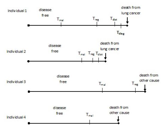
Figure A.1 presents four possible individual trajectories predicted by the MILC model. According to these trajectories, only Individual 1 and Individual 2 die from lung cancer, while only the first one is diagnosed before death. Individual 3 and Individual 4 die from some other cause, while at regional and local tumor stage respectively. Estimates of lung cancer related outcomes can be obtained by aggregating multiple simulated trajectories, either for the same individual or for a sample of people.

Examples of individual trajectories generated by the MILC model.
References
-
1
Multistate statistical modeling: A tool to build a lung cancer microsimulation model that includes parameter uncertainty and patient heterogeneityMed Decis Making 36:86–100.
-
2
Multi-state statistical modelling to quantify an individual-based micro simulation model for radiotherapy treatment in lung cancer patientsValue in Health 16:A325–A325.
-
3
Statistical methods in micro-simulation modeling: Calibration and predictive accuracyStatistical methods in micro-simulation modeling: Calibration and predictive accuracy, Doctoral dissertation, Brown University, https://repository.library.brown.edu/studio/item/bdr:386153/, (Biostatistics Dissertations, Brown Digital Repository.
-
4
MILC: Microsimulation lung cancer (MILC) model [Computer software manual]MILC: Microsimulation lung cancer (MILC) model [Computer software manual], Retrieved from , http://CRAN.R-project.org/package=MILC, (R package version 1.0).
-
5
Comparative Analysis of Calibration Methods for Microsimulation ModelsComparative Analysis of Calibration Methods for Microsimulation Models, Manuscript in preparation.
-
6
Assessing the Predictive Accuracy of Microsimulation ModelsAssessing the Predictive Accuracy of Microsimulation Models, Manuscript in preparation.
-
7
Turning gray: The natural history of lung cancer over timeJournal of Thoracic Oncology 3:781–792.
-
8
Uncovering the effects of smoking: historical perspectiveStatistical Methods in Medical Research 7:87–117.
-
9
Performance of the cancer risk management model lung cancer screening module [Journal Article]Health Rep 26:11–8.
- 10
-
11
Bridging population and tissue scale tumor dynamics: a new paradigm for understanding differences in tumor growth and metastatic disease [Journal Article]Cancer Res 74:426–35.
-
12
Maximum-likelihood estimation of the parameters of the gompertz survival functionJournal of the Royal Statistical Society. Series C (Applied Statistics) 19:152–159.
-
13
The natural history of lung cancer: a review based on rates of tumour growthBr J Dis Chest 73:1–17.
- 14
-
15
The miscan simulation program for the evaluation of screening for diseaseComputer Methods and Programs in Biomedicine 20:79–93.
-
16
Multistage carcinogenesis and lung cancer mortality in three cohortsCancer Epidemiology Biomarkers & Prevention 14:1171–1181.
- 17
-
18
Analysis of a historical cohort of chinese tin miners with arsenic, radon, cigarette smoke, and pipe smoke exposures using the biologically based two-stage clonal expansion modelRadiation Research 156:78–94.
-
19
Some properties of the hazard function of the two-mutation clonal expansion modelRisk Analysis 17:391–399.
-
20
Estimating age, period and cohort effects using the multistage model for cancerStatistics in Medicine 13:23–41.
-
21
A model for the effect of cigarette smoking on lung cancer incidence in connecticutStatistics in Medicine 15:565–580.
-
22
Survival analysis: techniques for censored and truncated dataSurvival analysis: techniques for censored and truncated data.
-
23
Advances in microsimulation modeling of population health determinants, diseases, and outcomesEpidemiology Research International, Article ID 584739.
-
24
Validation of population-based disease simulation models: a review of concepts and methods [Journal Article]BMC Public Health 10.
-
25
Breast-cancer - relationship between the size of the primary tumor and the probability of metastatic disseminationBritish Journal of Cancer 49:709–715.
-
26
A simulation model of the natural history of human breast cancerBr J Cancer 52:515–524.
- 27
-
28
Simulation modeling and tobacco control: creating more robust public health policies [Journal Article]Am J Public Health 96:494–8.
-
29
A simulation model of policies directed at treating tobacco use and dependenceMedical Decision Making 22:6–17.
-
30
A survey of dynamic microsimulation models: uses, model structure and methodology [Journal Article]International Journal of Microsimulation 6:3–55.
-
31
Policy assessment of medical imaging utilization: methods and applicationsPolicy assessment of medical imaging utilization: methods and applications, Unpublished doctoral dissertation, Harvard University.
-
32
The mgh-hms lung cancer policy model: Tobacco control versus screeningRisk Analysis 32:S117–S124.
-
33
Comparative analysis of 5 lung cancer natural history and screening models that reproduce outcomes of the nlst and plco trials [Journal Article]Cancer 120:1713–24.
-
34
Two-event model for carcinogenesis: Biological, mathematical, and statistical considerationsRisk Analysis 10:323–341.
-
35
Toward a new comprehensive international health and health care policy decision support toolOECD.
-
36
A new type of socio-economic systemThe Review of Economics and Statistics 39:116–123.
-
37
A natural history model of stage progression applied to breast cancerStatistics in Medicine 26:581–595.
- 38
-
39
An evidence-based microsimulation model for colorectal cancer: Validation and application [Journal Article]Cancer Epidemiology Biomarkers & Prevention 19:1992–2002.
- 40
-
41
Markov-models in medical decision-making - a practical guideMedical Decision Making 13:322–338.
-
42
Rates of growth of pulmonary metastases and host survivalAnnals of Surgery 159:161–171.
-
43
Growth kinetics of tumours : cell population kinetics in relation to the growth and treatment of cancerOxford: Clarendon Press.
-
44
[Web Page]. Retrieved from“Lung and Bronchus Cancer Statistics”, [Web Page]. Retrieved from, https://cancerstatisticscenter.cancer.org/#/cancer-site/Lung°/o20and°/o20bronchus.
-
45
International agency for research on cancer. Tobacco smokingIARC Monographs on the Evaluation of Carcinogenic Risks to Humans, 38.
-
46
[Web Page]. Retrieved from“Cancer Staging”, [Web Page]. Retrieved from, https://www.cancer.gov/about-cancer/diagnosis-staging/staging.
-
47
[Web Page]. Retrieved from“Harms of cigarette smoking and health benefits of quitting”, [Web Page]. Retrieved from, https://www.cancer.gov/about-cancer/causes-prevention/risk/tobacco/cessation-fact-sheet.
-
48
Frequency of first metastatic events in breast cancer: Implications for sequencing of systemic and local-regional treatmentJournal of Clinical Oncology 17:2649–2658.
- 49
-
50
The evaluation of health policies through dynamic microsimulation methodsInternational Journal of Microsimulation 5:2–20.
Article and author information
Author details
Acknowledgements
The author is deeply grateful to Dr. Carolyn M. Rutter and Dr. Constantine A. Gatsonis for the inspiration to specialize in micro-simulation modeling, and the very helpful comments on this manuscript; Dr. Samir S. Soneji for calculation of the CIF survival estimates based on real data; Dr Arlene Ash and Dr Kate Lapane for their useful comments that improved clarity. The reviewers’ comments which have considerably improved the final version of this manuscript. The work presented in this paper constitutes part of the author’s PhD research, conducted with support received from the American College of Radiology Imaging Network (ACRIN) (grant number: U01-CA-79778 from the National Cancer Institute).
Publication history
- Version of Record published: December 31, 2017 (version 1)
Copyright
© 2017, Chrysanthopoulou
This article is distributed under the terms of the Creative Commons Attribution License, which permits unrestricted use and redistribution provided that the original author and source are credited.