Solving a Partial Equilibrium Model in a CGE Framework: The Case of a Behavioural Microsimulation Model
- Productivity Commission, Australia
Cite this article
as: X. Zhang; 2017; Solving a Partial Equilibrium Model in a CGE Framework: The Case of a Behavioural Microsimulation Model; International Journal of Microsimulation; 10(3); 27-58.
doi: 10.34196/ijm.00165
- Article
- Figures and data
- Jump to
Figures
Figure 1

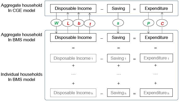
Variables linking the BMS and the CGE models.
Notes: Variables L, b, t and C are exogenous changes imported from the BMS model to the CGE model, while variables W, s and P are exogenous changes imported from the CGE model to the BMS model.
Figure 2a

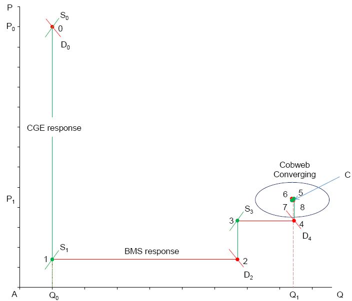
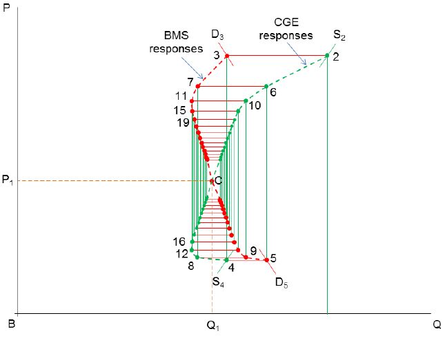
Convergence in the goods market: import tariff changes.
Figure 2b
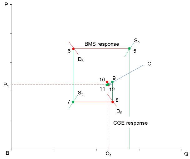
Cobweb converging toward equilibrium in goods market: import tariff changes.
Figure 3a

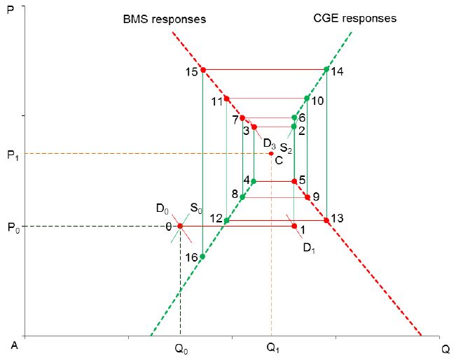
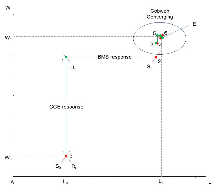
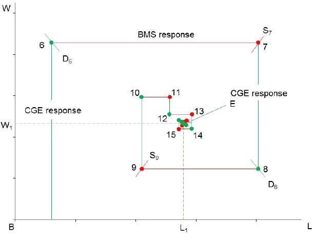
Diverging responses in the goods market without a slack variable: labour supply increase in the BMS model.
Figure 3b

Cobweb converging toward equilibrium in the goods market with saving rate as a slack variable.
Figure 4

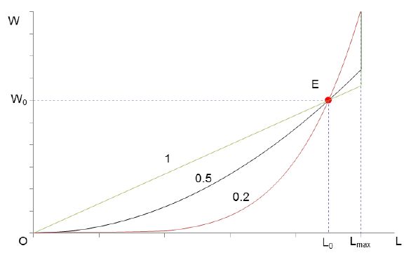
Labour supply curves with various elasticities.
Figure 5a

Converging process in labour market: import tariff changes from CGE model to BMS model with flexible labour supply.
Figure 5b

Cobweb converging toward equilibrium in labour market: import tariff changes with flexible labour supply.
Figure 6

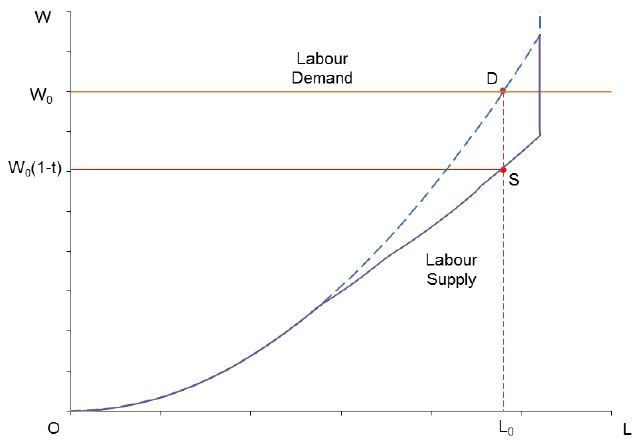
Effects of income tax on labour supply of an individual person.
Figure 7a

Converging process in labour market: marginal tax changes from BMS model to CGE model with flexible labour supply.
Figure 7b

Cobweb converging toward equilibrium in labour market: marginal tax changes with flexible labour supply.
Tables
Table 1
Income tax schedule and simulated changes.
| Income range ($) | Initial tax rates (%) | Simulated changes (%) | New tax rates (%) |
|---|---|---|---|
| 0 - 18,200 | 0 | 0 | 0 |
| 18,201 - 37,000 | 19 | 5 | 19.95 |
| 37,001 - 80,000 | 32.5 | 5 | 34.13 |
| 80,001 -180,000 | 37 | 10 | 40.70 |
| 180,001 and above | 45 | 10 | 49.50 |
-
Source: Australian Taxation Office (https://www.ato.gov.au/rates/individual-income-tax-rates/accessed 1 April 2016) and author calculations.
Table B.1
Aggregated input-output table in basic prices (AUD million).
| 1 ind | 2 hou | 3 gov | 4 inv | 5 stk | 6 exp | 7 mgn | Total | |
|---|---|---|---|---|---|---|---|---|
| 1 dom | 1,159,672 | 566,012 | 265,156 | 327,917 | −2,034 | 270,578 | 272,793 | 2,860,094 |
| 2 imp | 167,734 | 79,915 | 2,878 | 63,035 | 3,387 | 316,949 | ||
| 3 mgn | 94,733 | 127,542 | 2,672 | 20,227 | −87 | 27,706 | 272,793 | |
| 4 GST | 3,624 | 37,415 | 0 | 8,235 | 0 | 1,090 | 50,364 | |
| 5 tax | 17,831 | 25,502 | 0 | 13,609 | 652 | 0 | 57,594 | |
| 6 sub | −6,636 | −5,463 | 0 | −1,154 | −14 | −616 | −13,883 | |
| 7 fac | 1,371,108 | 1,371,108 | ||||||
| 8 ptx | 52,028 | 52,028 | ||||||
| Total | 2,860,094 | 830,923 | 270,706 | 431,869 | 1,904 | 298,758 | 272,793 | 4,967,047 |
-
Notes: Basic values of imports (316,949) include import tariffs (3,233).
-
Source: Compiled from Australian National Accounts: Input-Output Tables, 2012–13 (ABS 5209.0.55.001).
Table B.2
Sources of household income in CGE model and HES-SIH.
| CGE model | Household Expenditure Survey (HES-SIH) | |
|---|---|---|
| Wages for eight occupations (same as those in HES-SIH) | Managers and administrators; | Clerical and administrative workers; |
| Professionals; | Sales workers; | |
| Technicians and trade workers; | Machinery operators and drivers; | |
| Community and personal service workers; | Labourers; | |
| Capital | Own unincorporated business; | Superannuation/Annuity/Private pension and other regular sources |
| Investment; | ||
| Transfer payments from government | Austudy/Abstudy | Partner allowance |
| Age pension | Service pension | |
| Carer allowance | Sickness allowance | |
| Carer payment | Special benefit | |
| Disability pension | War widows pension | |
| Disability support pension | Widow allowance | |
| Family tax benefits | Wife pension | |
| Newstart allowance | Youth allowance | |
| Other pensions and allowances | Utilities allowance | |
| Overseas pensions and benefits | Senior supplement | |
| Parenting payment | Pension supplement | |
| Baby bonus payment; | ||
| Direct taxes | Income taxes | |
-
Source: Australian Bureau of Statistics, 2012.
Table B.3
Comparison between CGE and HES-SIH aggregates (AUD million).
| CGE data | HES-SIH scaled | HES-SIH | |
|---|---|---|---|
| (1) | (2) | original | |
| Expenditure | 830,924 | 830,924 | 609,468 |
| Income | 1,371,109 | 850,486 | 623,816 |
| Labour income | 744,282 | 744,282 | 545,918 |
| – Managers & administrators | 132,202 | 132,202 | 96,968 |
| – Professionals | 229,510 | 229,510 | 168,341 |
| – Technicians & trade workers | 101,273 | 101,273 | 74,282 |
| – Community & personal service | 45,706 | 45,706 | 33,525 |
| – Clerical & administrative workers work s | 91,417 | 91,417 | 67,052 |
| – Sales workers | 43,234 | 43,234 | 31,712 |
| – Machinery operators & drivers | 50,821 | 50,821 | 37,277 |
| – Labourers | 50,118 | 50,118 | 36,761 |
| Capital income | 626,826 | 154,400 | 113,250 |
| Benefits (23) | 106,875 | 78,391 | |
| Income Tax (-) | 155,071 | 113,742 | |
| Savings | 540,185 | 19,562 | 14,348 |
-
Notes: 1. Capital income in the input-output table is divided between household (154,400) and firm saving (472,426). 2. Scaling factor between columns (2) and (3) = 1.3634.
Table C.1
Sets used in the model and database.
| Sets | Definitions |
|---|---|
| COM(1,…,m): | Commodities (indexed by c) |
| IND(1,…,m): | Industries (indexed by i) |
| MCM(1,…,n): | Margin commodities (indexed by m) |
| NCM(= COM - MCM): | Non-margin commodities (indexed by c) |
| FUSR(gov, hou, inv, stk): | Final users of commodities (indexed by u) |
| USR(=IND + FUSR): | Users of commodities (indexed by u) |
| USR_stk(=USR - stk): | Users of commodities, exclusive of stk (indexed by u) |
| SRC(dom, imp): | Domestic/import sources of commodities (indexed by s) |
| FAC(lab,cap): | Factors of production (indexed by f) |
| OCC(1,…,8): | Labour occupation (indexed by o) |
| SAV(inv,stk): | Saving destination (indexed by s) |
| HOU(1,…,9774): | Sample households (indexed by h) |
| PER(1,…,6): | Persons in a household (indexed by p) |
| B23(1,…,23): | Transfer payments (indexed by b) |
| TAX(GST, tax, sub): | Three tax items (indexed by g) |
Download links
A two-part list of links to download the article, or parts of the article, in various formats.