Spatial competition with interacting agents
- Cornell University, United States
- Augustana College, United States
- Sorbonne University, France
- Northwestern University, United States
- Article
- Figures and data
- Jump to
Figures

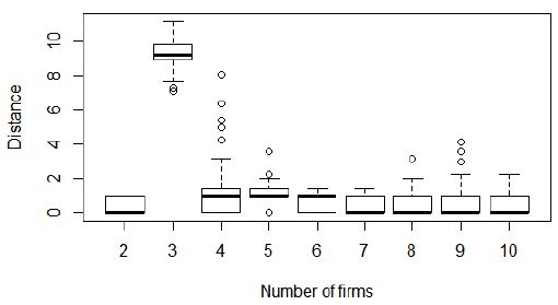
Minimum distance to nearest when firms choose locations but prices are fixed.
Notes: Data plotted from 500 replicate simulation runs for each case (2 through 10 firms).
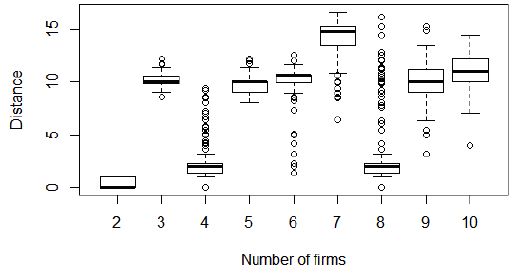
Maximum distance to nearest firm when firms choose locations but prices are fixed.
Notes: Data plotted from 500 replicate simulation runs for each case (2 through 10 firms).

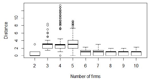
Minimum distance to nearest firm when firms choose both prices and locations.
Notes: Data plotted from 500 replicate simulation runs for each case (2 through 10 firms).
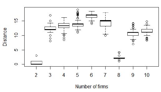
Maximum distance to nearest firm when firms choose both prices and locations.
Notes: Data plotted from 500 replicate simulation runs for each case (2 through 10 firms).

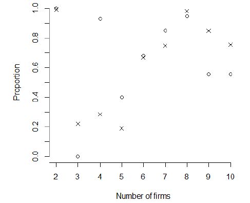
Proportion of firms that form local duopoly pairs (less than 3 units distance from one other firm at the end of the simulation run).
Notes: Circles mark the case when firms choose locations but prices are fixed. Crosses mark the case when firms choose both locations and prices. Each data point represents the mean value from 500 replicate simulation runs.

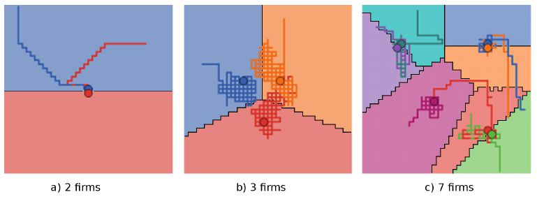
Characteristic locations with two, three and seven firms when firms choose locations but prices are fixed.
Notes: Firms are represented by circles, each filled in with a distinct color. The grid cells, each representing a customer, are colored using a lighter shade of the same hue as the firm which they currently patronize. The history of firms’ movement is shown as a trail of corresponding color.

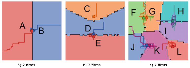
Characteristic locations with two, three and seven firms when firms choose both prices and locations.
Notes: Visualization of firms and customers’ patronage is the same as described in Figure 6 above.

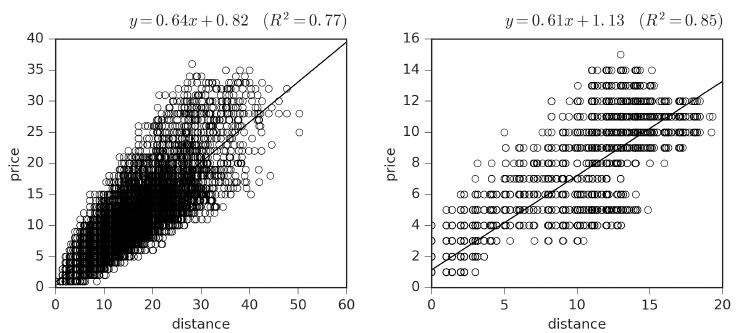
Price versus distance to nearest competitor when firms choose prices but locations are fixed (left panel) and when firms choose both locations and prices (right panel).
Notes: Data plotted from each firm from all of the 4500 simulations involving 2 to 10 firms.

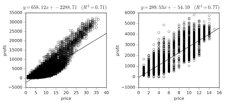
Profit versus price when firms choose prices but locations are fixed (left panel) and when firms choose both locations and prices (right panel).
Notes: Data plotted from each firm from all of the 4500 simulations involving 2 to 10 firms.

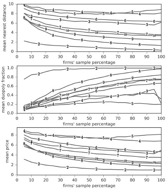
Sensitivity analysis for the distance between nearest firms (top panel), the fraction of firms involved in local duopolies (middle panel), and the average price (bottom panle), with respect to firms’ sampling percentage (what fraction of consumers each firm surveys about potential patronage during decision-making).
Notes: Each data point represents the average across 500 simulation runs on a 41x41 grid.
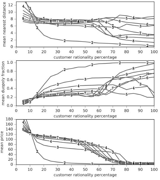
Sensitivity analysis for the distance between nearest firms (top panel), the fraction of firms involved in local duopolies (middle panel), and the average price (bottom panel), with respect to customer rationality (the percent chance that each customer will choose to patronize their minimal cost firm, instead of choosing randomly among all firms).

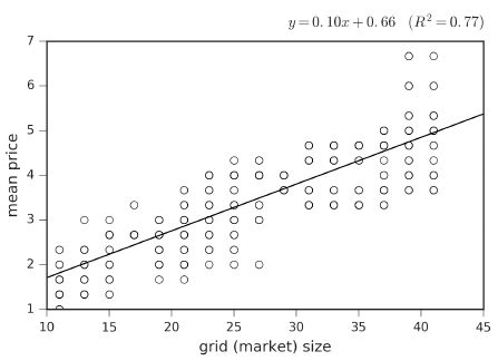
Average price versus grid size for 3 firms that are choosing both location and price.
Notes: Results shown are from 50 replicate simulations for each grid size, which ranged from 11 to 41 by increments of 2.
Tables
Pseudocode for the agent-based model.
| Initialization: |
| customer agents placed on each lattice point of 41x41 grid. |
| for each firm Fi ∈ F1, F2, …, FN: |
| place firm Fi on a random lattice point. |
| set initial price for Fi ← 10 |
| Each time step: |
| let M (the set of movement actions) = |Up, Down, Left, Right} |
| let P (the set of price change actions) = |+1,-1} |
| for each firm Fi: |
| Fi selects mi ∈ M s.t. calculatedProfitAfter(mi) is maximized |
| Fi selects pi ∈ P s.t. calculatedProfitAfter(pi) is maximized |
| for each firm Fi: |
| Fi takes actions mi and pi |
| for each customer Cj: |
| Cj selects firm Fmin s.t. price(Fmin) + transportationCost(Fmin, Cj) is minimized. |
| Cj purchases one unit of the good from Fmin |
Selling prices for the firms shown in Figure 7.
| Region | A | B | C | D | E | F | G | H | I | J | K | L |
| Price charged | 1 | 1 | 8 | 2 | 2 | 2 | 2 | 3 | 3 | 2 | 3 | 10 |
-
Notes: Firms positioned farther apart from others (e.g., C and L) charge higher prices than firms in competitive local duopolies, because they are able to raise prices without losing as many customers as firms who have nearby competitors.