A top-down with behaviour (TDB) microsimulation toolkit for distributive analysis
- Partnership for Economic Policy (PEP), Université Laval, Canada
- CEDLAS-UNLP and Partnership for Economic Policy (PEP), Argentina
- Partnership for Economic Policy (PEP), Kenya
- Article
- Figures and data
- Jump to
Abstract
Computable General Equilibrium (CGE) models are often combined with microsimulation (MS) models to perform distributive impact analysis for fiscal or structural policies, or external shocks. This paper describes a user-friendly Stata-based toolkit to perform MSs combined with CGE models in a top-down fashion. The toolkit is organized in various modules, which can be easily adapted to the users’ needs. It first estimates income generation by type of work and skill of workers. Then it estimates households’ specific price deflators based on individual utility. The changes estimated by a CGE model (or from other sources) in the employment (by skill and sector), in the wage payroll (by skill), in the revenues from self-employment activities (by skill) as well as in the commodities prices are fed into the MS model in a consistent way. Once the new vector of real consumption or revenue is estimated, it performs a series of distributive analysis, such as the computation of standard poverty and inequality indices, their decomposition by income factor, robustness analysis and growth incidence curves, and compare the baseline with the simulation results. This makes it possible to run standard poverty and distributive analyses, and to see whether a given shock or policy has had some impact on household welfare and who are the most affected households. Based on such information, social protection policies can be accurately designed in order to minimise the, for example, negative effects of a given shock in a cost-effective manner. An illustrative analysis is run on data from Uganda.
1. Introduction
The toolkit we describe in this paper is particularly intended for researchers who aim at estimating a microsimulation (MS) model combined with a Computable General Equilibrium (CGE) model. Nonetheless, it may also be used to simulate the microeconomic effects of exogenous changes coming from other sources (for example, macro projections, hypothesised shocks, etc.). Very generally, a MS model is a model of the behaviour of individual agents (individuals, households, firms). As such, it can be used to simulate the effects of economic policies or other shocks on those individual agents. In this article, we focus on the impacts on individuals and households. To the best of our knowledge, this is the first attempt to make a similar toolkit publicly available, including an example application to real data.
The main objective of the MS model presented in this paper is to simulate changes in per capita household income/welfare under various (counterfactual) scenarios. The simulation results are then used to conduct standard poverty and distributive analyses of these changes and make policy recommendations. For example, in the case of negative shocks, social protection policies can be accurately designed to target the most affected households/individuals in order to minimise the negative effects in a cost-effective manner.
As mentioned above, we will focus on the particular case where the MS model draws information on the shock variables from a CGE model. This type of combined CGE-MS models has been used widely to evaluate the distributive impacts of macroeconomic shocks and policies such as public expenditures (changes in size or composition), tax/subsidy policies, structural reforms such as trade liberalization, privatization and labour market reforms, and global price shocks. The toolkit we propose here performs MSs combined with a CGE model in a top-down fashion. The toolkit is organized in various and distinct modelling modules, which can be easily adapted or augmented according to the users’ needs. This toolkit can be particularly relevant for development practitioners willing to conduct distributive impact analyses of macroeconomic shocks, but also to academics as a starting point for developing similar toolkits with alternative MS modelling. The toolkit is implemented in Stata because it is probably the most-used statistical software by development practitioners and distributive analysts, and also because —to run the distributive impact analysis— it uses the Distributive Analysis Stata Package (DASP) (Araar & Duclos, 2007), one of the best-known package for distributive analysis.
The idea to link macro (including CGE) and MS models for this purpose emerged in the mid-1980s (inter alia, Meagher & Agrawal, 1986 examined the impacts of changes in the existing tax mix on the distribution of income in Australia). CGE models allow the modeller to focus on winners and losers at the sectoral level, and to estimate the impact on macroeconomic variables and general equilibrium price effects. However, they are not an adequate tool to perform distributional analysis given the lack of individual/household results and the representative agent assumption (that is, the household in a CGE model is an aggregate household and not an average household).
On the other hand, MS models focus on household and/or individual behaviour. They are the key methodology to capture distributional effects of a policy change due to heterogeneity at the household or individual level. However, they are not able to capture the economy-wide effects of macro shocks (international trade, tax policy, public expenditures, etc.). Furthermore, they lack general equilibrium effects. If the macro shock or policy is substantial, there will likely be consequences for income distribution, sectoral prices, factor returns, employment, labour supply, GDP, etc., which are not captured by a MS model alone. For example, the reform of a tax-benefit system is likely to affect labour supply which, in turn, may affect wages and prices. Even in cases where the shock impacts are at the micro level (for example, a cash transfer programme), if it is on a large scale it is likely to have significant macro repercussions (for example, changes in labour force participation, changes in household consumption) that may, in turn, feed back to the micro impacts.
In outline, we proceed as follows. Section 2 describes alternative approaches to CGE-MS analysis. Section 3 presents our behavioural top-down CGE-microsimulation model. Section 4 summarizes our Stata code for the MS model. Section 5 exemplifies how the results from a CGE-MS model run can be interpreted. Section 6 concludes the paper.
2. Computable general equilibrium–microsimulation approaches: some general features
There are several major categories of CGE-MS models found in the literature (see Cockburn, Savard, and Tiberti (2014) for a comprehensive review): (1) the representative household group approach; (2) the fully integrated approach; (3) the top down micro-accounting approach; (4) the top-down with behaviour approach; (5) the bottom-up approach; and (6) the top down/bottom up or iterative approach.
The toolkit presented here is based on the top-down with behaviour approach, which is probably the most widespread framework in this literature. This approach basically consists in taking results from a CGE model —such as changes in prices, factor returns, employments levels, etc.— and feeding them into a MS model. Generally, through a micro-econometric estimation, it introduces behaviours for labour supply (see Robilliard, Bourguignon, & Robinson, 2008), consumption and savings. A top-down “microsimulation” approach is illustrated in Figure 1.
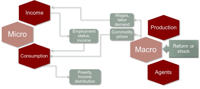
Illustration of a typical “top-down” microsimulation approach.
For most of the approaches listed above, some preliminary work is required to ensure compatibility between the CGE and MS models in terms of data and modelling hypotheses. Ideally, we should calibrate the national accounts data (used in the CGE model) and household data (used in the MS model) in order to reach “empirical consistency”. For example, Robilliard and Robinson (2003) propose a method to reconcile these data by modifying the sampling weights. Also, we must harmonize the categories (labour, commodities, products, sectors, etc.) and functional forms (for example, consumer demand) for the two layers (macro and micro).
However, when a sequential approach is followed, “full consistency is not required between the macro and the micro sides of the model. Indeed, all of the analysis using this model may be performed in terms of deviations from benchmarks that may not fit perfectly together” (Robilliard et al., 2008, p. 106). It should also be noted that the household or individual behaviour in the MS model often lacks the theoretical consistency of the CGE model. For example, in MS models, for occupational choices relative prices rarely enter the utility function.
The top down with behaviour approach: TD-WB
In the literature, MS models combined with CGE models follow two main approaches: parametric or non-parametric. The parametric approach generally involves a system of equations that determine occupational choice, returns to labour and to human capital, household purchasing power and other household (individual) income components. The non-parametric approach generally involves seeking individuals with similar characteristics to simulate certain changes (for example, a change in labour income for an individual that moves from unemployment to employment), and occupational shifts that may be proxied by a random selection procedure within a segmented labour market structure. In this article, we adopt a parametric approach, which is the most common in the literature and, we believe, as long as the behavioural parameters are correctly estimated, it better captures observed individual behaviour. However, as shown by Debowicz (2016), parametric and non-parametric MS approaches to CGE-MS modelling lead to consistent and similar results.
Under this approach, imperfect labour markets and occupation allocation models are introduced. Also, econometric models of household income are estimated, allowing for full individual heterogeneity. In particular, we distinguish different sources of income and individual occupational choice, and we estimate the individual consumer utility function.
The MS model is linked by applying the changes simulated by the CGE model for the following linkage aggregate variables (LAVs): wages, prices, production volumes, and structure of employment by labour market segment. Ideally, under this framework, the household data underlying the MS model should be used to estimate key parameters of the CGE model (for example, consumption demand). The MS model is then used to simulate the effect on household income of modifying a subset of variables in accordance with the results of the CGE model (for example, not only wages, prices, other revenues —as under the accounting approach— but also employment status). Finally, to ensure consistency, we check that changes in LAVs match with the changes in average values of the corresponding variables in the MS model. This can be done by: introducing elasticities of labour supply that can also be used to model aggregate labour supply in the CGE model (see Bourguignon & Savard, 2008); recalibrating (for example, changing the intercepts of the behavioural equations of MS model, as in Robilliard et al., 2008); ranking the individuals according to their estimated probabilities associated to each labour behaviour to change their status consistently with the macro employment results as in Cockburn, Robichaud, and Tiberti (in press) — (more description of the latter is provided below); imposing consistency equations (as in Colombo, 2010).
This approach makes it possible to introduce rich behaviour and a fair amount of heterogeneity between households by capturing extensive margin and intensive margin changes in labour supply, and discrete choices by individuals or households. Nonetheless, such an approach has some limits such as the absence of a micro-feedback effect to the CGE model. The magnitude of this problem is linked to the size of the aggregation error from the micro households up to the aggregate households in the CGE model.
Introducing dynamics
These models normally keep key household characteristics (demographics, school participation, etc.) constant. Dynamic simulations, in the form of repeated simulations of the household income-generation model for period-specific changes in the shock variables, would require adding a population-ageing model to the MS model. For instance, this may require a MS model that ages the population over time using estimated or calibrated functions for fertility, mortality, migration, marriage, household formation, schooling, etc. (see for example Grimm, 2005). It is useful to consider that, when combined with a dynamic CGE, the MS model should take into account the evolution of the population. This can be done by “sampling re-weighting” techniques or by changing the attributes of the individuals. We can in fact distinguish between “static ageing” (sampling re-weighting) and “dynamic ageing”. Under the former, sampling weights are modified so that the simulated population matches the macro aggregates. This approach is usually used in the short-to-medium run as no significant alteration in the population structure is expected. A well-known technique is the algorithm developed by Deville and Särndal (1992). With the “dynamic ageing” technique, real life events (for example, birth, death, etc.) are modelled and, based on that, individual and household characteristics are updated at each period. These approaches are often combined with calibration mechanisms to align micro aggregates with macro forecasts.
3. Top-down with behaviour computable general equilibrium-microsimulation: description of the methodology
In what follows, we briefly discuss each of the modules included in the toolkit. Two main models are presented below: income generation and consumption. Full details are provided in Tiberti, Cicowiez, and Cockburn (2017).1
3.1 Income generation model: Employment and income
Under a behavioural microsimulation approach, individuals and households adjust different types of behaviour. In the CGE-MS literature, most of the contributions focus on the modelling of labour markets and incomes from working activities.
This module ultimately aims at estimating the variations in household welfare due to changes in employment status and the categories of workers based on their skills and the economic sectors. Also, we need to establish the degree of rigidities to the labour market (for example, degree of mobility of workers across the different occupational choices), identify the best suited function for the occupational choice and revenues, and estimate them. Finally, for each simulation period, we predict the individual employment status as well as the corresponding earnings, and estimate the total household income.
Occupational status
Given that we generally do not have good data on the number of hours worked, the labour supply by a household member is defined as a discrete choice among alternatives. In the illustrative example presented below, the occupational choices (statuses) available to household members are: (1) wage worker; (2) self-employed in non-agriculture; (3) farmer; (4) not working (which also includes unemployed and apprentices). As is commonly done with multiple discrete choices, the individual labour supply is estimated with a standard multinomial logit model,2 where each choice is then modelled within a discrete utility-maximizing framework. The utility associated with each possible category is a function of a set of individual and household characteristics. The model we use to estimate the individual labour supply (Ei) is a reduced-form model in the sense that earnings (in each of the three working alternatives) do not enter the estimation of the labour supply. The residuals are drawn randomly from the Gumbel distribution up to when the set of these values is in accordance with the observed occupational choices by following the methodology described in Bourguignon, Fournier, and Gourgand (2001).
The labour supply is estimated separately by categories of workers based on their individual education skills. In the application below, we have (1) skilled (if they completed at least primary education); and (2) unskilled (if their education level being lower than completed primary education). Workers can be employed in one of the three sectors as identified above (wage, non-agricultural and agricultural). Concerning the labour mobility hypotheses, consistently with the CGE model, in each period, each worker can potentially reassess his/her utility of being in one of the three categories and eventually become a wage worker, farmer or non-agricultural self-employed. However, his/her choice is finally determined by individual and household characteristics.
After the probabilities associated with each occupational status are estimated, we can proceed with assigning the new individual employment status. Differently from Robilliard et al. (2008), this is done by a “job queuing” approach. According to the CGE results concerning the employment status, the absolute number of workers moving in or out the three working categories is estimated. The individuals changing from one alternative to another are selected according to their probability of being in the relevant occupational category.
As mentioned above, the CGE results need to be plugged into the MS model in a consistent manner: that is, the share of each working category in the CGE model and the MS model must be the same in each simulated period. In the illustration below (Figure 2), we assume perfect mobility across sectors (wage workers can move to non-farm, farm self-employment or not employed, and vice versa), and perfect rigidity across type of workers (unskilled workers cannot move into the skilled pool, and vice versa).
Income from working activities
We then move to the estimation of individual and household incomes. Individual wages are estimated through the Mincer model and is estimated by a two-step procedure (Heckman model). We first estimate the “selection equation” (that is, being in the wage sector or not) and then the “wage” equation. In addition, we estimate the individual unobserved fixed effects (or, heterogeneity of individual earnings). While its estimation is immediate for individuals employed in the wage sector at the base (observed) year, for individuals who did not report information on wages (that is, nonwage workers), this residual term is estimated by drawing randomly from a normal distribution with the relevant (for example, skilled or unskilled) observed variance. Finally, we can integrate the variations in the wage rates as predicted by the CGE. Note that changes in average wages (that is total payroll) with respect to the baseline figures in the MS must be equal to changes in wages obtained in the CGE model for each type of worker category.
Household profit (farmers and non-agricultural self-employed workers) is estimated through an instrumental variable approach as some explanatory variables —for example number of family workers— may be endogenous and thus correlated with the error term.
The basic model for household profit is estimated through a Cobb-Douglas function. Then, similarly to wages, we need to recover the error term both for those households who reported a positive profit value during the base year and for those with missing values. Again note that after the simulations, only the deterministic component of the model is recomputed (by using the regression parameters estimated at the base year). The estimated household profit (including the residual terms) is finally divided by the total number of household members (skilled and unskilled) working in the farm or in the non-agricultural family enterprise.
The changes in profits from farming and non-agricultural self-employment activities as simulated by the CGE are then fed into the MS model. The changes in net income from self-employment activities in the MS must be equal to changes in income per worker in non-agricultural and farming sectors resulting from the CGE model.
We can finally estimate the total household income at time t (Yh,t) as:
where the first component on the right-hand side is the total income from wages summed at the household level (for all household members i = i, …, N) for skilled (s = H) and unskilled (s = L) wage workers, and I(.) is simply an indicator function taking value one if individual i is employed (E = 1) as a skilled or unskilled wage worker at time t, and 0 otherwise. The second component represents the total household profit
We can then easily calculate the relative change of income between the base year and period t as:
which is then applied to total household consumption to estimate the change in total income. The value we obtain is then added to our welfare variable (in most contexts, this is the initial expenditure variable) (see Section 3.2 below). In such a way, we implicitly assume that there is no change in the marginal savings rate. Another reason for following this strategy is that the resulting change in income is compatible with the expenditure variable. This would not necessarily be the case if we add the estimated absolute change in income.
3.2 Household consumption and prices
This module serves to estimate the predicted change in real household consumption. We are then able to estimate the variation in poverty and inequality for each simulation period. The change in real consumption comes from the variation in household incomes (as derived in the previous modules) and consumer prices.
Per capita consumption at constant prices is our variable of interest to estimate changes in poverty and inequality across the different simulation scenarios. The first step is to define the categories of commodities available from the household survey. These categories are determined by mapping the categories in the underlying micro and macro data and then aggregating by nature of commodity. To take into account the heterogeneity of the effect of price changes across households, it is important to calculate a household-specific price index. To do so, we relied on King’s (1983) approach to define the concept of “equivalent income”. The toolkit models households’ preferences with a Cobb-Douglas utility function. Once the household specific price deflator is derived, the equivalent income is estimated.
The new vector of real household income (after the simulation) is ready to run standard “poverty and distributive analysis”.3 For the purpose of poverty and distributive analysis, we used the standard poverty gap indices and the Gini inequality index. We also run some stochastic dominance analysis to assess the robustness of our results throughout the simulation period.
Finally, we analyse the poverty decomposition by income sources (notably, wages, profits and consumer prices) and the growth incidence curves. Decomposition by income source is performed using the Shapley/Shorrocks approach (for more details, see Shorrocks, 2013; and Azevedo, Inchauste, Olivieri, Saavedra, & Winkler, 2013). The growth incidence curve is a useful tool to have an overall picture of impacts over the whole distribution. It is estimated as the difference of the logarithm of the welfare variable under the simulation and the baseline scenarios at each percentile of the distribution (see Ravallion & Chen, 2003).
3.3 Final methodological remarks
As discussed, the estimations of employment and incomes include some random terms. This implies that the household income for the counterfactual scenarios is random. We proceeded by replicating each simulation a sufficiently large number of times (100 times). Then, we took the median values of these 100 replicates for each relevant estimator (namely, per adult equivalent income, and poverty and inequality indices) in each simulated year, and estimated their corresponding confidence intervals.
4. Feeding the microeconomic model and how to use the stata codes
In this section we describe how the MS model presented in Section 2 can be implemented with a given set of shocks (for example those obtained from a CGE model) in order to obtain poverty and inequality results. In particular, we explain how this approach is implemented in Stata.
In our MS model, the labour market and consumer prices are considered to be the main transmission channels of the impact of the simulated policy or exogenous shocks scenarios on poverty and income inequality. For example, individuals may change position in the labour market (and hence also affect household income) due to external shocks, trade reforms, or other policy changes. In turn, workers may shift from one sector to another, change occupation or lose their jobs. From a practical point of view, the methodological issue is to find a procedure that can account for such labour-market shifts and identify which individuals are most likely to shift position in order to be able to simulate a new, counterfactual income distribution. In addition, our MS model also considers changes in commodity prices through a household-specific consumer price index.
In a nutshell, for a number of variables of the labour and commodity markets (that is, changes in skilled and unskilled employment and wages, and changes commodity prices), changes for each year of the scenarios are calculated relative to a particular year, or base year of the MSs. As seen above, some of the results generated by the CGE model are fed into our MS model. More precisely, each scenario definition should provide changes with respect to the base year (that is 2010 with the example shown below) for the following variables: 1) employment (rural skilled employed, urban skilled employed, rural unskilled employed, urban unskilled employed), 2) wage payroll (skilled workers, unskilled workers), 3) income from self-employment activities (skilled workers, unskilled workers), and 4) (categories of) commodity prices.
4.1 Implementation in stata
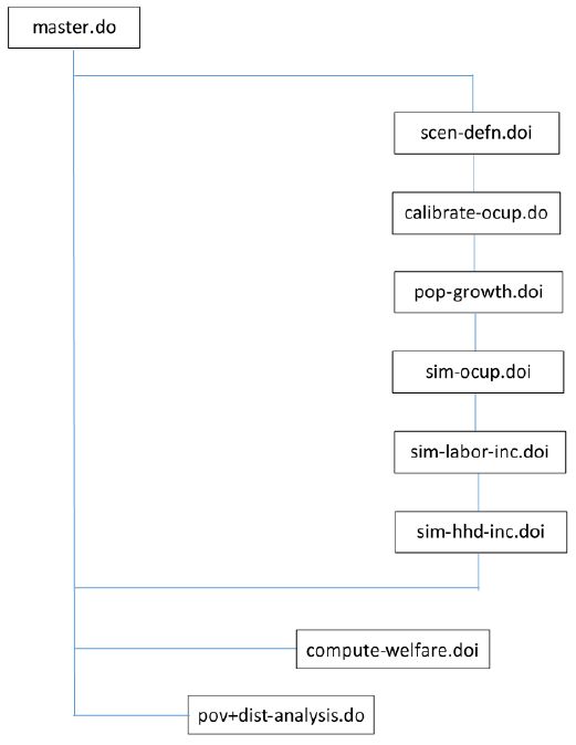
The MS toolkit is organised in three separate folders: “Do-Files”, “Output”, and “Raw-Data”. In the first one we have all Stata codes to run the MS as described in the figure below (Figure 2).

Organization of Stata codes in the MS model.
The output folder is where results are saved. These include data files, graphs and tables. In particular, the toolkit generates estimates for: poverty and inequality rates over time (baseline and simulation scenarios); poverty decomposition by income factors over time (simulation scenario with respect to the baseline); poverty and inequality rates, their difference between simulation and baseline scenarios and the confidence intervals over time; Foster-Greer-Thorbecke (FGT), FGT-difference and growth indicende curves
5. Interpreting the microeconomic results of a given shock
In what follows, we present the various poverty and distributive results generated by the toolkit. For this illustrative example, the simulation period is from 2011 to 2030. The variations fed into the MS model have been estimated through a CGE model, which simulated the baseline scenario and a policy scenario simulating large investments in the oil sector in Uganda. For the baseline simulation, forecast data (regarding GDP growth and population growth) from the International Monetary Fund (IMF) are used. Regarding the policy scenario, the first phase of the simulation (2015–2017) concerns large investments in the oil sector when there is no production from this sector. This is followed up with a construction phase from 2018–2030. In this second phase, the oil sector generates production, and profit and labour income generated in the oil sector goes to Ugandan households. It is also in this phase that profits and labour payments are generated. In this simulation, we assume that that foreigners fund the investment in the oil sector (as a “gift” from the rest of the world to Uganda).
As said earlier, the main goal of the MS component is to estimate the impacts on households and individuals. In particular, we want to identify the most affected and advantaged population groups in the distribution following the proposed investment in the oil sector.
As shown in Figure 3, the poverty rate and poverty gap decrease along the whole simulation period. However, their trajectory differ between the baseline and the simulation scenarios. As for the simulation setup, the two scenarios do not differ until 2014. As said earlier, the simulated policy intervention starts in 2015. The short to medium term impact on household welfare and poverty is negative, as detected by the upward jump in 2015 (or year 5 of the simulation) for both the incidence of poverty and the poverty gap. Specifically, the proposed investment would cause a rise in the incidence of poverty by 2.5 percentage points and by around 1.3 percentage points in the poverty gap. In other words, such a policy would push back the poverty indicators to their 2010 value. In the long term, the baseline and reference scenarios tend to converge.

Evolution of the FGT0 and FGT1 between 2010 and 2030.
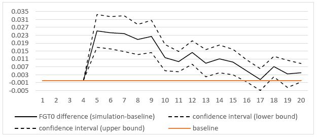
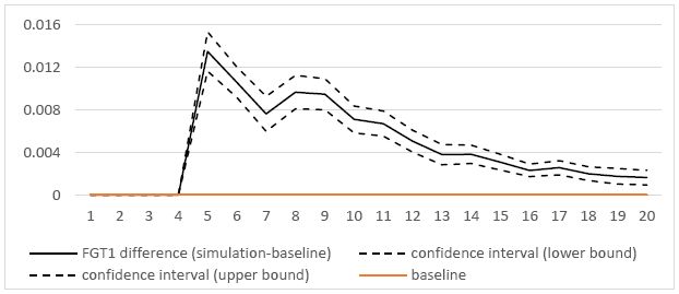
According to Figure 4a, the poverty headcounts in the two scenarios are not statistically different starting from 2027 (or year 17), with the only exception of 2028 (where the poverty rate is significantly higher in the simulation scenario). In contrast, as shown in Figure 4b, the poverty gap under the simulation scenario is always statistically higher than in the baseline along the whole period, although the difference approaches zero near the end. The policy intervention also has a negative impact on inequality (Figure 4c). The effects are higher when the oil sector starts to produce and to generate income (that is from 2018) and slowly decrease over time, but being always statistically significantly higher than under the baseline.

Difference between the FGT0 under the simulation and the baseline.

Difference between the FGT1 under the simulation and the baseline.
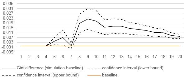

Difference between the Gini under the simulation and the baseline.
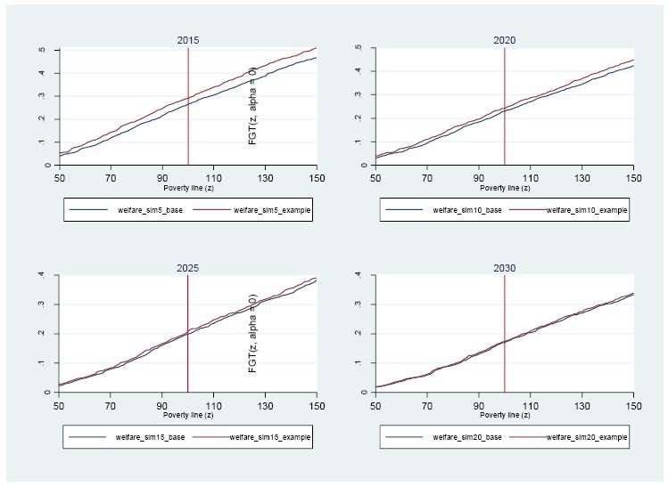
Our results are robust over a large range of possible poverty lines. As shown in Figure 5, the FGT0 curve associated to the baseline always dominates (that is, lies below or poverty is lower than) the simulation FGT0 curve. In a separate analysis, we found (see “cfgts2d” graphs) that for the majority of poverty lines in the adopted range, the difference between the simulation and baseline curves are statistically different from zero. As said earlier, starting from 2017, the baseline curve does not clearly dominate the simulation curve.

FGT0 curves for selected years (5, 10, 15 and 20).
As discussed above, the proposed policy intervention would particularly affect households during the first years of implementation. Out of a total increase by 2.5 percentage points in 2015 between the simulation and baseline scenarios, Figure 6 shows that 3.2 points are attributable to the large rise in consumer prices due to the investment. While the simulated changes in the income from the agricultural and non-agricultural sectors do not substantially affect the poverty difference, variations in wage would reduce poverty under the simulation scenario (with respect to the baseline) by around 0.5 points. Between 2016 and 2021, the change in agricultural income would negatively affect poverty (with respect to its baseline counterfactual); after that, it would slightly decrease or have no effects on poverty. Income from non-agricultural self-employment would help —though marginally (0.2–0.4 points a year)— decrease poverty from 2018. Wages would help to reduce poverty along the entire period by 0.2 to 0.8 points a year. Consumer prices are the major factor of the increase in headcount poverty in the whole period, even if their (negative) contribution decreases over time, falling from a contribution of 3.2 points in 2015 to 0.8 points in 2030.

Decomposition of FGT0 by income factors.
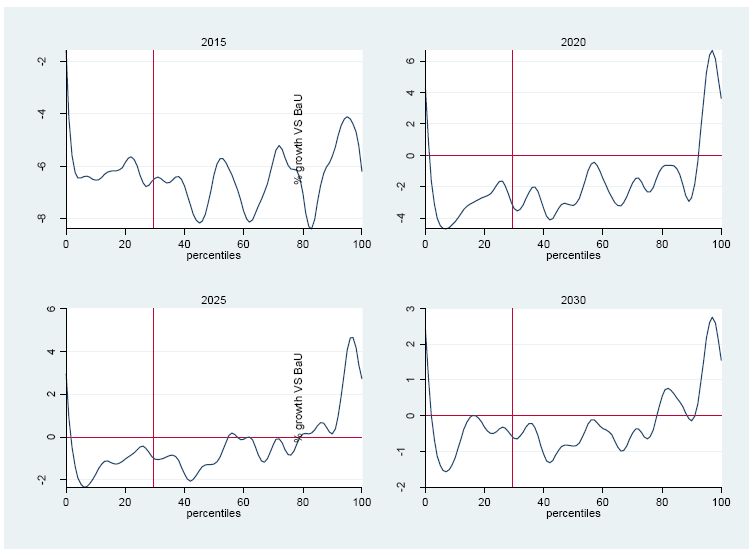
Finally, we propose to look at the distributive effects along the whole distribution for some selected years. This is done by using Growth Incidence Curves, which draw the percentage change of consumption under the simulation scenario (with respect to the baseline — normalised to zero in the graphs below) for all the percentiles in our population. As shown by Figure 7, soon after the policy implementation (in 2015), all percentiles would be negatively affected. The change in consumption is indeed always negative, with those in percentiles 40th to 80th being particularly affected (up to -8%), and with those below the poverty line experiencing a 6% reduction. In later periods, richer percentiles (around the top 10%) would have higher income than under the baseline; in contrast, lower percentiles would continue to experience some reduction, though at a smaller rate over time (about -3% in 2020, -2% in 2025 and -1% in 2030) and without significant differences between those lying below the poverty line and those above. Overall, the results shown below confirm an increase in inequality over time, with a rise by 0.8 points by 2030.

Growth Incidence Curves for selected years.
6. Conclusions
In this paper we introduced a new user-friendly Stata-based toolkit (TDB) to perform MSs combined with CGE models in a top-down fashion. TDB’s main features include the estimation of the income generation and welfare variables for all sampled households for the baseline and simulation scenarios, consistently with CGE (or other macro sources) generated results. TDB’s main final outputs are standard poverty and distributive indicators and graphs resulting from the introduction of a given shock or policy. TDB’s main goal is to help understanding the direction and the magnitude of the impact of a given shock or policy on households along the whole income distribution. Based on such information, social protection policies can be accurately designed in order to minimise the, for example, negative effects of a given shock in a cost-effective manner. An illustrative example of the toolkit was provided on data from Uganda.
Footnotes
1.
2.
we are aware that, with this approach, we do not control for the potential selection in the estimation of income (from wage and profits) associated to each occupational alternative (this issue may be solved by using, for example, the method developed in Bourguignon, Fournier, & Gourgand, 2007). However, for profits we only have information at the household level and we prefer not to decompose it into individual values (for more details, see below in the text).
3.
Poverty and distributive estimates, as well as significance tests and dominance curves, are carried out using the Distributive Analysis Stata Package (DASP) (Araar & Duclos, 2007).
Appendix
List of indicators estimated by the toolkit:
- Poverty and Inequality rates over time, baseline and simulation scenarios (Sheet distindic):
time = simulation period
FGT0_base = poverty rate for baseline
FGT0_example = poverty rate for non-base simulation
FGT1_base = poverty gap rate for baseline
FGT1_example = poverty gap rate for non-base simulation
Gini_base = Gini coefficient for baseline
Gini_example = Gini coefficient for non-base simulation
- Poverty decomposition by income factors over time, simulation scenario with respect to the baseline (Sheet fgtdecomp):
time = simulation period
welfare = zero by definition (as it serves as benchmark value in the baseline)
wage = contribution of wage changes to overall change in welfare
nonWageNonAg = contribution of non-wage non-agricultural income to overall change in welfare
nonWageAg = contribution of non-wage agricultural income to overall change in welfare
CPI = contribution to (household-specific) price changes to overall change in welfare
Total
- Poverty rates, difference between simulation and baseline scenarios and confidence intervals over time (Sheet difgtindic):
time = simulation period
FGT0_base = poverty rate for baseline
FGT0_example = poverty rate for non-base simulation
diff = absolute difference between FGT0_base and FGT0_example
standardDev = standard deviation of diff
lowBound = lower bound for diff
upperBound = upper bound for diff
FGT1_base = poverty gap rate for baseline
FGT1_example = poverty gap rate for non-base simulation
diff = absolute difference between FGT1_base and FGT1_example
standardDev = standard deviation of diff
lowBound = lower bound for diff
upperBound = upper bound for diff
- Inequality, difference between simulation and baseline scenarios and confidence intervals over time (Sheet diginiindic):
time = simulation period
gini_base = Gini for baseline
standardDev_base = standard deviation of Gini for baseline
gini_example = Gini for non-base simulation
standardDev_example = standard deviation of gini for non-base simulation
diff = absolute difference between FGT0_base and FGT0_example
standardDev_diff = standard deviation of the difference
lowBound_diff = lower bound for diff
upperBound_diff = upper bound for diff
- FGT, FGT-difference and growth indicende curves (stored in the Output\Graphs folder):
file cfgt-tgph = FGT curves (along an axis of poverty lines) for simulation period t
file cfgts2d-t.gph = differences between FGT poverty curves with confidence interval for simulation period t
file cnpe-tgph = growth-incidence curve for simulation period t, estimated using parametric regression curves
References
-
1
DASP: Distributive Analysis Stata Package, PEPUNDP and Université Laval: World Bank.
-
2
Is Labor Income Responsible for Poverty Reduction? A Decomposition Approach. Working Paper No. 6414Washington DC: World Bank Policy Research.
-
3
Selection Bias Corrections Based On The Multinomial Logit Model: Monte Carlo ComparisonsJournal of Economic Surveys 2:174–205.
-
4
Fast Development with a Stable Income Distribution: Taiwan, 1979-94Review of Income and Wealth, International Association for Research in Income and Wealth 47:139–63.
-
5
The Impact of Macroeconomic Policies on Poverty and Income DistributionA CGE Integrated Multi-Household Model with Segmented Labour Markets and Unemployment, Eds., The Impact of Macroeconomic Policies on Poverty and Income Distribution, The World Bank, Oxford University Press.
-
6
Energy Subsidy Reform and Poverty in Arab Countries: A Comparative CGE-Microsimulation Analysis of Egypt and JordanReview of Income and Wealth, 68, S1.
-
7
Handbook of Microsimulation Modelling275–304, Macro-Micro Models, Handbook of Microsimulation Modelling, Contributions to Economic Analysis, 293, Emerald Group Publishing Limited.
-
8
Linking CGE and Microsimulation Models: A Comparison of Different ApproachesInternational Journal of Microsimulation 3:72–91.
-
9
Does the microsimulation approach used in macro–micro modelling matter? An application to the distributional effects of capital outflows during Argentina’s Currency Board regimeEconomic Modelling 54:591–599.
-
10
Calibration Estimators in Survey SamplingJournal of the American Statistical Association 87:376–382.
-
11
Educational policies and poverty reduction in Côte d’IvoireJournal of Policy Modeling 27:231–247.
-
12
Welfare analysis of tax reforms using household dataJournal of Public Economics 21:183–214.
-
13
Taxation reform and income distribution in AustraliaAustralian Economic Review 19:33–56.
- 14
-
15
The Impact of Macroeconomic Policies on Poverty and Income DistributionExamining the social impact of the Indonesian financial crisis using a macro-micro model, The Impact of Macroeconomic Policies on Poverty and Income Distribution, The World Bank, Oxford University Press.
-
16
Reconciling household surveys and national accounts data using a cross entropy estimation methodReview of Income and Wealth 49:395–406.
-
17
Decomposition procedures for distributional analysis: a unified framework based on the Shapley valueJournal of Economic Inequality 11:99–126.
-
18
A top-down with behaviour (TDB) microsimulation toolkit for distributive analysis. Working Papers PMMA 2017-24Partnership for Economic Policy (PEP).
Article and author information
Author details
Acknowledgements
The authors would like to thank Luc Savard, Véronique Robichaud and Jean-Yves Duclos for their insightful help, comments and discussions. Financial support from Oxford Policy Managament (OPM) is greatly acknowledged (Contract Name: 5198 – Development of an Integrated Macro Economic Model for the Government of Uganda; PO Number: 5198 / PO10155). We also acknowledge the financial support from the Partnership for Economic Policy (PEP), with funding from the Department for International Development (DFID) of the United Kingdom (or UK Aid), and the Government of Canada through the International Development Research Center (IDRC).
Publication history
- Version of Record published: August 31, 2018 (version 1)
Copyright
© 2018, Tiberti et al.
This article is distributed under the terms of the Creative Commons Attribution License, which permits unrestricted use and redistribution provided that the original author and source are credited.