Using trajectory analysis to test and illustrate microsimulation outcomes

Cite this article as: J. Salonen, H. Tikanmäki, T. Nummi; 2019; Using trajectory analysis to test and illustrate microsimulation outcomes; International Journal of Microsimulation; 12(2); 3-17. doi: 10.34196/ijm.00198

Article
Figures and data
Jump to

Abstract

We propose a new data-driven way of testing and visualizing dynamic microsimulation outcome data. The proposed statistical methodology is based on trajectory analysis (Nagin, 1999), which can be used to identify several sub-populations from a population measured longitudinally. We briefly introduce the statistical basis of trajectory analysis and discuss its use in the context of microsimulation. Finally, we report our results from the Finnish microsimulation model ELSI (Tikanmäki et al., 2014; Tikanmäki et al., 2015) to illustrate the possibilities and benefits of this technique. Trajectory analysis is available in many statistical software packages (e.g., SAS, R, Stata and Mplus). We conclude that trajectory analysis is a useful tool for investigating microsimulation outcomes.

1. Introduction

This paper has two goals. First, we present a statistical technique called group-based trajectory analysis and demonstrate its usefulness in a microsimulation context. We use trajectory analysis to identify unknown groups or sub-populations that can yield valuable information that is not necessarily easily accessible by other means. Second, we use three examples to show how this technique, among others, can be used to validate models and to reveal possible misspecification of the microsimulation model.

Trajectory analysis has recently gained much popularity in a number of fields including psychology, criminology (Nagin and Odgers, 2010; Nagin, 2016; van der Geest et al., 2016), sociology (Hynes and Clarkberg, 2005; Don and Mickelson, 2014), education (Kokko et al., 2008), marketing (Mani and Nandkumar, 2016) and health sciences (Nummi et al., 2014; Nummi et al., 2017a). It has increasingly been used in studies on labor market attachment (Peutere et al., 2015; Nummi et al., 2017b). To our knowledge, trajectory analysis has very seldom been used in a microsimulation context.

Dynamic microsimulation results are often reported using some ex ante classification (e.g., education, age, or labor market state). The trajectory approach offers key advantages over ex ante classification, which stem from the a priori use of an economic taxonomy. The basic advantage of trajectory analysis is that it can reveal latent patterns in longitudinal data that might otherwise remain hidden, hence complementing ex ante classifications. Furthermore, the use of a formal statistical methodology has the capacity to distinguish chance variation across individuals from real differences caused by latent sub-groups (Nagin and Odgers, 2010).

In this paper, we propose two kind of trajectory analysis implementations. First, the data can be stratified by various background factors (e.g., by labor market state) and thus the latent sub-groups are to be found within the strata. This would yield information on, for example, how common the earnings trajectories (by population state) are in the stratas investigated. Second, another way would be to classify the trajectory groups by some background factor after trajectory analysis. This would yield information on how the ex ante classifier (e.g., labor market state) is divided in trajectory groups.

Population heterogeneity is an important topic in dynamic microsimulation. Credible heterogeneity in a simulated population is a desired property of any microsimulation model. Trajectory analysis is a powerful method for demonstrating this heterogeneity. It allows for the analysis of any microsimulation outcome with interesting population heterogeneity. For instance, in the Finnish ELSI model we could analyze the individual population state, pension contributions, working lives or incomes. The technique is especially suited to cohort-based analysis, but it can also handle several cohorts simultaneously.

The approach we propose has a number of advantages. First, trajectory analysis has the potential to reveal interesting sub-groups of individuals. Second, the technique of trajectory analysis with normal distribution (like other members of the exponential family) is a well-established method, with software packages readily available for microsimulation practitioners (e.g. Jones et al., 2001; Leisch, 2004; Grun and Leisch, 2007; Haughton et al., 2009; Muthén and Muthén, 2010). Third, trajectory analysis is a flexible method that can be applied to both cross-sectional data (single period measurements), and more importantly, to longitudinal data (multiple periods of measurements). The most common metric for indexing time is age or year. Another possible metric would be time before or since a life-event.

Descriptive analysis is often inadequate for the purposes of empirical research. Trajectory analysis can provide a more rigorous examination with time-dependent covariates or risk factors affecting trajectory group membership (Nagin, 2005; Jones and Nagin, 2007). In addition to single outcome analysis, trajectory analysis also allows for the simultaneous analysis of multiple outcomes Nagin et al., 2016). Indeed, there is now a growing body of research that uses multiple trajectory analysis (e.g. Hsu, 2015; Nummi et al., 2017b). Nummi et al. (2017b) provide an example of the simultaneous modeling of employment, education, unemployment and parental leaves using a multivariate trajectory model. These abovementioned extensions also provide interesting possibilities for microsimulation data analysis.

The method has also its disadvantages. First, trajectory analysis can only be performed with discrete-time data. Most dynamic microsimulation models are defined in discrete-time, with time-point intervals of one year (Zaidi and Rake, 2001; Li and O’Donoghue, 2013; Li et al., 2014). This leads to a second disadvantage, which can be described as state vs. event microsimulation. Trajectory analysis is easiest to implement with the calendar year as the time interval, that is, using state microsimulation models.

Trajectory analysis is often applied to normally distributed data, but it is also applicable to discrete distributions such as binomial, Poisson, multinomial, etc., making this method a useful tool for the exploratory analysis of data sets. In this paper, we show three examples of trajectory analysis in microsimulation contexts. These examples cover labor market simulation topics such as wage earnings, education and pensions. Trajectory analysis of these outcomes illustrates the technique with different data distributions.

2. Trajectory analysis in microsimulation

2.1. Trajectory analysis

Trajectory analysis is, in essence, the application of finite mixture modeling to longitudinal data. It can be used for modeling the unobserved heterogeneity of individuals measured longitudinally (e.g. Nagin, 1999; Nagin, 2005). In what follows we describe the statistical background for our application of trajectory analysis.

The statistical foundation of trajectory analysis is on finite mixture modeling. Well-established in the field of statistics, the mixture modeling method concerns modeling a statistical distribution by a mixture (or weighted sum) of distributions (see Titterington et al., 1985; McLachlan and Peel, 2000). Böhning et al. (2007) give examples of the use of finite mixture modeling in various statistical applications.

Two basic modeling approaches are called growth mixture modeling and group-based trajectory modeling. They share the same analytical objective of measuring and explaining differences across population members in their developmental course. The difference between approaches lies in the way they model individual-level heterogenity in developmental trajectories.

Growth mixture models depict the average trend of outcome and individual-specific variation around the average trend with random effects using the same parameters of change (Nagin and Odgers, 2010).

Our specific aim is to identify individuals or objects in microsimulation data with the same kind of unknown developmental profiles (trajectories or sub-groups). The microsimulation population is then splitted into several sub-populations. Let $y_{i} = {(y_{i 1}, y_{i 2}, \dots, y_{i T})}^{'}$ represent the sequence of measurements on an individual i over T periods and let $f_{i} (y_{i} | X_{i})$ denote the marginal probability distribution of $\boldsymbol{y}_{i}$ with possible time-dependent covariates $\boldsymbol{X}_{i}$ . It is assumed that $f_{i}\left (\boldsymbol{y}_{i}|\boldsymbol{X}_{i}\right)$ follows a mixture of K densities

f_{i} (y_{i}| X_{i}) = \sum_{k = 1}^{K} π_{k} f_{i k} (y_{i}| X_{i}), \sum_{k = 1}^{K} π_{k} = 1 w i t h π_{k} > 0,

where $π_{k}$ is the probability of belonging to the sub-group k and $f_{ik}\left (\boldsymbol{y}_{i}|\boldsymbol{X}_{i}\right)$ is the density for the kth sub-group. Trajectory analysis can handle discrete or continuous data. The simplest choice is to use the Bernoulli distribution {0, 1} for the mixture components $f_{ik}\left (\boldsymbol{y}_{i}|\boldsymbol{X}_{i}\right)$ : but other members of the exponential family are often applied as well. It is assumed that given kth sub-group measurements are independent. For Bernoulli mixtures we can write

f_{i k} (y_{i} | X_{i}) = \prod_{t = 1}^{T} p_{i t k}^{y_{i t}} (1 - p_{i t k}^{1 - y_{i t}}),

where the probability $p_{itk}$ is a function of covariates $\boldsymbol{X}_{i}$ . For modeling the conditional distribution of $p_{itk}$ we use the logistic regression model. For the ith individual, we can then use the equation

p_{i t k} = \frac{e x p (x_{i}^{`} β_{k})}{1 + e x p (x_{i}^{`} β_{k})},

where $\boldsymbol{x}_{i}^{`}\left (t\right)$ is the tth row of $\boldsymbol{X}_{i}$ and $\boldsymbol{\beta }_{k}$ is the parameter vector for the kth sub-group. For the analysis of continuous data, one alternative is the multivariate normal distribution

f_{i k} (y_{i} | X_{i}) = {(2 π)}^{- \frac{p_{i}}{2}} | Σ_{i k} |^{- \frac{p_{i}}{2}} e x p {- \frac{1}{2} {(y_{i} - μ_{i k})}^{'} Σ_{i k}^{- 1} (y_{i} - μ_{i k})},

where $\boldsymbol{\mu }_{ik}$ is a function of covariates $\boldsymbol{X}_{i}$ with parameters $\boldsymbol{\beta }_{k}$ and $Σ_{i k} = σ_{k}^{2} I$ a covariance matrix within kth sub-group. Thus, the measurements are assumed to be independent within sub-group k, with the variance $\sigma _{k}^{2}$ . One advantage of this assumption is that it considerably simplifies the likelihood function and thus yields a computationally lighter and more stable analysis.

For modeling the trajectory mean in time t, simple linear models are usually applied, e.g. low-degree polynomials. For our three examples we used cubic polynomial model

x^{`} β_{k} = β_{0 k} + β_{1 k} t + β_{2 k} t^{2} + β_{3 k} t^{3}

to model the development within the sub-group k in time (age). The mean model can also include other time-dependent covariates or time-stable covariates (risk-factors).

For parameter estimation, Maximum Likelihood (ML) estimates can be calculated by maximizing the log-likelihood $\sum \limits_{i=1}^{N}f_{i}$ over unknown parameters $β_{i k}$ and $\sigma _{k},\ k=1,\ldots ,K$ (see e.g. Nagin, 1999; Jones et al., 2001; Jones and Nagin, 2007). In most software packages, the method used for ML estimation is the EM (Expectation and Maximization) algorithm (see Dempster et al., 1977; McLachlan and Peel, 2000). The algorithm in an iterative technique involving two steps. E step finds the expected log likelihood under current parameter estimates, the subsequent M step maximizes the expected log likelihood function. These steps are iterated until the estimates converge. When applied to trajectory analysis, the E step calculates the posterior probability for sub-group membership

w_{i k} = \frac{π_{k} f_{k} (y_{i} | X_{i}, \emptyset_{k})}{f (y_{i} | X_{i}, \emptyset_{k})}

under all parameter estimates ${\hat{\emptyset}}_{k}$ . The estimated sub-group probabilities are then

{\hat{π}}_{k} = \frac{1}{N} \sum_{i = 1}^{N} {\hat{w}}_{i k}

Once the model parameters have been estimated, the posterior probability estimates provide a way to assign each individual to a specific sub-group or trajectory. Individuals can be assigned to the specific sub-group in which their posterior probability is highest. From the equations, we see that the assignment of individuals into groups takes into account regression parameter estimates, the number of groups, probability distribution, membership probability estimates and time span of longitudinal dataset. These are major topics in trajectory analysis and need careful consideration from microsimulation practitioner. Nagin (2005) discusses the selection of the number of groups (p. 78–87) and related statistical information criteria (p. 63–76) and the question of conditional independence (p. 26–27).

The question of groups as real entities is discussed in Nagin and Odgers (2010) and Nagin (2016). Nagin (1999) discusses the use of group membership probabilities in the calculations, as well as the links between group membership probabilities and other time-dependent covariates besides age (or time). The nature of trajectory groups in growth mixture modeling and group-based trajectory analysis is discussed in Nagin, 2005, pp. 54–56), Nagin (2016) and Nathalie et al. (2017). Don and Mickelson (2014) discuss the good practices of trajectory analysis, especially in terms of model selection.

Note that the sub-groups revealed by trajectory analysis are not fixed constructs. They are just approximations of a more complex reality. Each individual belong to a specific group with a certain probability. It would be good if we could investigate the fit of the assumed model using the identified trajectory groups. However, since the groups are based on maximum posterior probability, this would probably introduce some correlation to within-group residuals, as the actual group could also contain individuals from other groups with a small probability or weight. The correct approach from a statistical point of view, however, would be based on the investigation, using alternative covariance structures (for example, likelihood-ratio type test statistics or some other information criterion). However, this kind of testing is impossible in Nagin’s basic model. This topic has been discussed in Nagin and Odgers (2010) and Nagin (2016).

As with any statistical analysis of dynamic microsimulation outcome data, a change in the period of observation would naturally change the results of the model. The trajectory groups could also be affected to a certain extent. However, we believe that in our examples the basic main grouping structure would remain quite similar.

2.2. Finnish ELSI microsimulation model

ELSI is a longitudinal microsimulation model (Tikanmäki et al., 2014; Dekkers and Van den Bosch, 2016) that is used to assess the development of the statutory pensions in Finland. The dynamic ageing model has been developed at the Finnish Centre for Pensions, a statutory co-operation body providing research and expertise services related to the Finnish pension system.

ELSI model has been designed to assess the future earnings-related pensions and the national pensions (Tikanmäki et al., 2017). It can also be used to analyze changes in the pension system and in the underlying demographic or macroeconomic conditions. One of its uses has been to assess the distributional effects of the pension reform of 2017 (Tikanmäki et al., 2015).

The Finnish pension system is mainly based on pension rights accrued on the basis of the individual’s life-time earnings. The only exception is the survivor’s pension, which accounts for no more than 6% of total pension expenditure. The ELSI model is therefore based on individual-level information and calculations of pensions received in one’s own right. The model comprises both pension recipients and those still working. The model simulates each individual’s working life prior to retirement.

The base population consists of all adults aged 18 or over covered by the social insurance system in Finland. Most of the material is drawn from administrative records maintained by the Finnish Centre for Pensions and the Social Insurance Institution of Finland. Information on educational level from Statistics Finland is also added to the model. The ELSI model provides the opportunity to run large populations. For the present analysis we used a random sample of 32% of the base population, which in numerical terms translates into 1.5 million individuals in the baseline year of 2012. The population is then simulated until 2085. Deceased people remain in the model and a new cohort as well as new immigrants enter the model each year. Consequently the population increases over the course of the simulation.

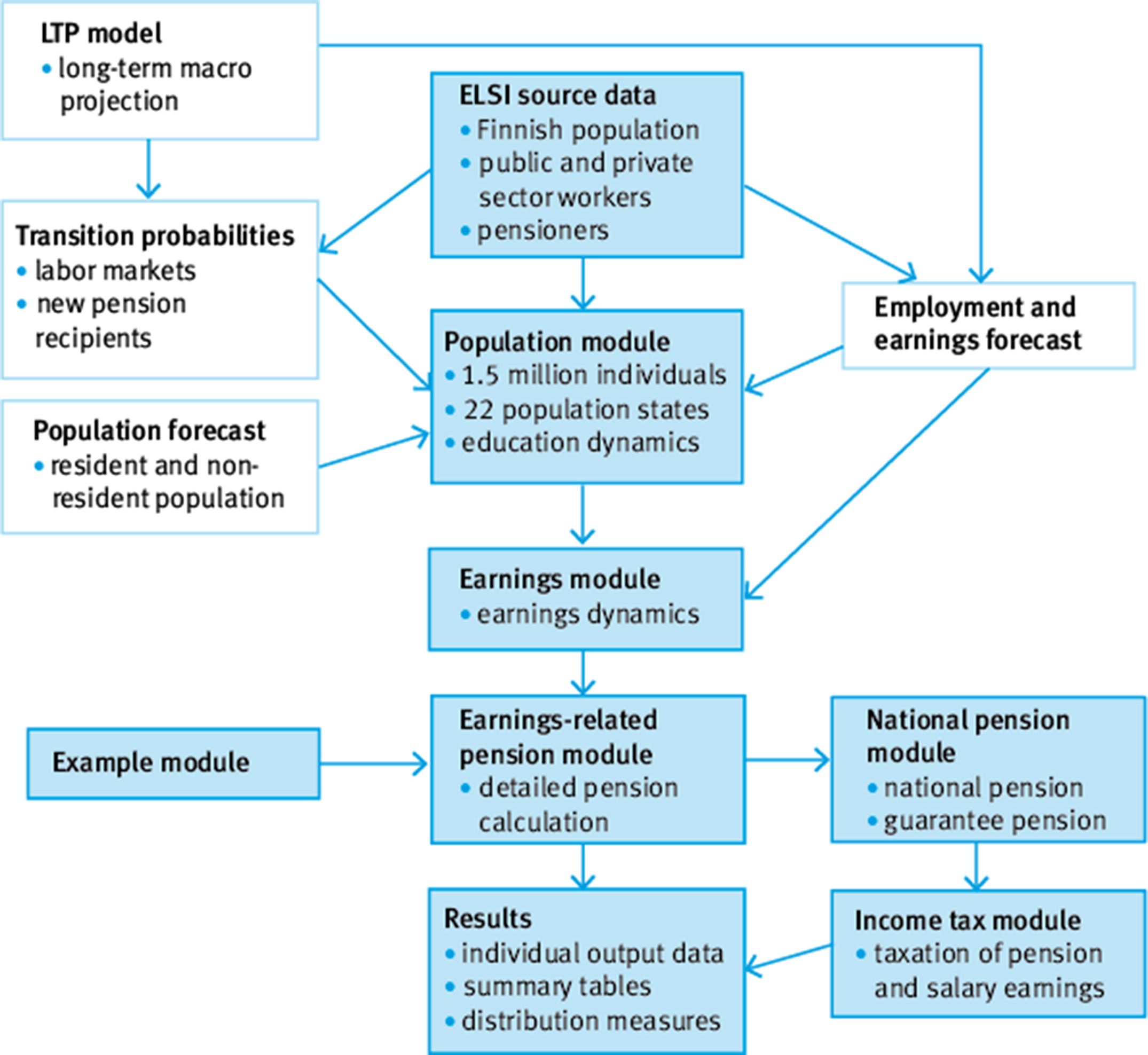
The ELSI model has a modular structure (Figure 1). Each colored box represents a module of the model, while white boxes represent external sources of information. There are no feedback loops from later to earlier modules. The simulation starts from the population module, followed by the earnings module, pension modules, and the taxation module, and finally brings together the results.

Figure 1

Download asset Open asset

Structure of the ELSI microsimulation model

The population module has several functions. It simulates population and labor market transitions as well as educational changes. The population module is based on transition probabilities that are estimated from historical data for 2010–2014. The module also uses Statistics Finland’s official population forecast to replicate general trends in the sample population. Transition probabilities, with one-year time steps, are by and large deterministic, that is, based on exogenous information.

In the population module, we simulate a new population or labor market state for each individual based on transition probabilities. There are 22 states in the model, the most important of which are: active (employed), inactive, unemployed, various pension states for different pension benefits, and deceased.

The labor market transitions are of Markovian type, which means that the transition probabilities are based on current state rather than former history. However, it is possible to add memory to a Markov process by extending the state space. For instance, in model ELSI we have three different active states. One for those employed first consecutive year, another for those employed second year and third one for the rest. Hence, unemployment risks may be higher for those who do not yet have an established labor market position.

Education is also simulated in the population module. Post-basic education dynamics is based on age and gender-specific transition probabilities. Changes in education level are possible at any age, although they are not very common after age 35.

The transition probabilities are updated each simulation year using the population level information produced by the semi-aggregated LTP model (Tikanmäki et al., 2017). There is thus a simple alignment of microsimulation outcomes to macro level aggregates.

Wage earnings are simulated in the earnings module. Wages are simulated for each individual annually based on the labor market state and an underlying earnings-equation, which is a time-series model with a stochastic component. The earnings equation takes also into account gender, age and level of education. Wages are simulated for active workers and those in partial retirement. The earnings module is described in Tikanmäki et al. (2014).

The earnings-related pension module calculates pension amounts based on the simulated time of retirement (retirement age) and life-course earnings. The pension calculation takes no shortcuts but is as detailed as possible given the data in use. The national pension and guarantee pension amounts are calculated as a residual of the earnings-related pension, since they are income tested. The calculation of national pensions is described in Sihvonen (2015).

The taxation module finalizes the substantive simulation. The previous modules have produced gross wages and pensions. In the taxation module, the current (2016) rules for income taxation are applied to both simulated wages and pension earnings. The calculation of income taxes is described in Sihvonen (2015).

After the simulation run, the results are analyzed in the results module, which calculates aggregate results over the course of the simulation, based on individual-level outcomes. Measures of the distribution (mean, percentage points, Gini coefficient) of pensions can be produced by ex ante classifiers such as gender, level of education and year of birth. Aggregate measures on the duration of working life and partition of life-course into active and passive stages are also calculated in the result module. The module collects individual-level output data containing information on labor market state, wage earnings, residence, education level, pension earnings, pension benefit, working life, pension accrual, etc. Therefore the material is also available for the statistical analysis illustrated in this paper. The proposed statistical technique could be used with many other outcomes as well.

In the following analysis we use a longitudinal individual-level data set that covers the period from 2008–2085 with a 25% sub-sample of the original output data. The analysis is based on three outcomes: wage earnings, education level and pension earnings. The wage and education trajectories are presented for the male cohort born in 1995 and pension trajectories for the male cohort born in 1960. With trajectory analysis, it would be possible to analyze several cohorts at the same time so long as the data is longitudinal.

Similar longitudinal data is produced in many other dynamic microsimulation models, too. For example, the Swedish SESIM model and the Norwegian MOSART model are in this respect similar to ELSI, providing rich individual or household level labor market output data (Fredriksen and Stølen, 2007; Klevmarken and Lindgren, 2008; Flood et al., 2012).

2.3. Trajectory model selection

Choosing the number of mixture components K is an important stage of finite mixture modeling. The trajectory method requires the researcher to specify the assumed number of sub-groups in the data. The optimal number of sub-groups K can be assessed using information criteria, which are widely used in this context.^[1] One commonly used criterion to assess the model fit is the Bayesian information criterion (BIC). The model with largest BIC is preferred (SAS implementation). One may also calculate the group-specific average posterior probability over individuals to measure the fit. If this values exceeds the minimum threshold (at least 0.7) the fit is considered satisfactory. Nagin (2005, p. 63–77) provides an overview of model selection in trajectory analysis context. Ultimately, meaningful real-world interpretations of sub-groups requires not just information criteria, but also theoretical evaluation and good judgment.

In trajectory analysis missing data is considered missing completely at random according to the taxonomy layed by Little and Rubin (1987). Software packages handle missing data in such a way that all available data is used in the estimation. In other words, all individuals or objects with some missing longitudinal data values are included in the analysis.

From Table 1 we can see the BIC values of our example analyses on three outcome-variables (earnings, education and pension). The BIC score indicates that, a five-group solution fits the wage earnings and pension variables, while for education BIC increases with more groups. However, increasing the number of education groups further would yield some infinitesimal groups. Therefore our choice is the five-group solution for the wage earnings and pension outcomes, and the six-group solution for the education outcome variable.

Table 1

BIC scores and number of sub-groups k

Outcome	3	4	5	6
Earnings (N=3,325)	−50288.7	−48178.8	−45974.7	−46375.9
Education (N=13,173)	−549399.6	−544342.9	−537412.2	−535026.8
Pension (N=10,761)	−834881.4	−811092.8	−786210.9	786234.1

Notes: BIC = log(L) −.5 * log(n) k, where L = log likelihood, n = sample size and k = number of parameters.

In this study the computations were carried out using SAS software package with accompanying PROC TRAJ application, an easy to use PC SAS procedure for analyzing Nagin’s model (e.g. Jones et al., 2001; Jones and Nagin, 2007; Andruff et al., 2009).^[2] Appendix A.1 gives an example of the programming code for wage earnings trajectories (Example 1, k=5).

The trajectory plots (Figures 2–4) present conditional means of time points calculated over the simulation period. Relative sizes ${\hat{π}}_{k}$ of the sub-groups are also presented in the figures. These plots are the main tool for interpreting the results obtained. The estimated model is summarized in Appendix (A.2), which includes group-specific parameter estimates. The SAS procedure also produces a confidence interval (95%) and model-predicted values by sub-group if necessary.

Figure 2

Download asset Open asset

Figure 3

Download asset Open asset

Figure 4

Download asset Open asset

It must be emphasized that the trajectories in the following examples are group means, which indicates that there is a range of individual tracks around the trajectory curves. Software packages routinely output the group estimates and confidence intervals to visualize within-group population heterogeneity. For the sake of readability, the model fit curves and confidence intervals are not presented in this paper.

In the examples we use cubic age model (see Equation 5). The choice depends on the assumed development of the data over time. One advantage in PROC TRAJ is that the age or time model can be group-specific, which means that for example one group can be fitted with a second order polynomial model, whereas another group can be fitted with a cubic model etc.

3. Examples

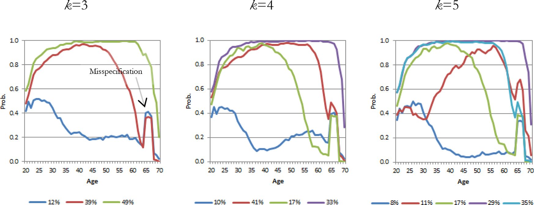
3.1. Earnings trajectories: binary outcome

For this example, we have chosen a young cohort to illustrate a simulated life-course. The cohort, born in 1995, enters labor markets at age 17 (year 2012), and subsequent life-course including individual wage earnings is simulated in the ELSI model’s population and earnings modules.

The example shows a trajectory analysis with binary outcome data. Individual yearly wage is dichotomized (yes = 1/no = 0), so wage earnings could also be interpreted as employment. In terms of content, wage earnings could be analyzed without transformations using continuous data (euros).

The BIC score (Table 1) indicates that a five-group solution yields the best fit for the earnings outcome, but we also present the solutions for three and four-groups solutions. Figure 2 shows that the relative sizes ${\hat{π}}_{k}$ vary somewhat with an increasing number of groups. Nevertheless all solutions have essentially the same major sub-groups.

In terms of content, we can see that there is a large group (k = 3: 49%, k = 4: 33% and k = 5: 29%) with strong labor market integration, or a strong earnings profile, until retirement age. Other groups show an early declining trend in employment. Labor market integration is weak in one group (k = 3: 12%, k = 4: 10% and k = 5: 8%), especially at older age. Unemployment and permanent disability draw individuals out of employment prior to old-age retirement. Retirement age for old-age pension in this cohort is 67 years and 9 months. Partial old-age pension can be drawn three years before retirement age.

3.1.1. ELSI model recalibration

This trajectory analysis experiment revealed a slight misspecification in the ELSI model’s earnings module (see spikes at age 65 in all trajectory solutions). The spikes are visible in mean-based trajectories, but they would not be seen in fitted means models. This goes to show how useful group-based mean curves can be in revealing model misspecification.

In the earnings module the mechanism for working after retirement did not work as intended. During the course of simulation, many of those who had stopped working earlier suddenly decided to return to work after drawing their pension (Figure 2). Of course, such behavior is not plausible on a larger scale.

The Finnish pension system allows full-time employment even after retirement on an old-age pension. However, wage earnings for old-age pensioners are typically quite low. The misspecification therefore did not have a major impact on the main results and was not observed in comparison with the LTP macro model.

In the ELSI model earnings are calibrated with the LTP model. In practice, this is done by comparing projected average earnings each year by gender, population state and age. Any deviations imply changes in the ELSI model’s parameters.

In the LTP model, working after retirement is not modeled in detail, and the relevant point of reference is provided by the corresponding statistical figures. In the ELSI model, the share of new retirees working after retirement is the same as in the observed statistics. Trajectory analysis showed that the pool of retirees working after retirement also included individuals who had not worked in the year preceding retirement, which was not intended.

Following the trajectory analysis of simulated earnings, the ELSI model was recalibrated appropriately. There was no change in the aggregate figures, namely wage sum and number of people working after retirement.

Trajectory analysis is not yet routinely part of ELSI model testing, but it could be incorporated as part of its validation procedures.

3.1.1.1. Composition of trajectory groups

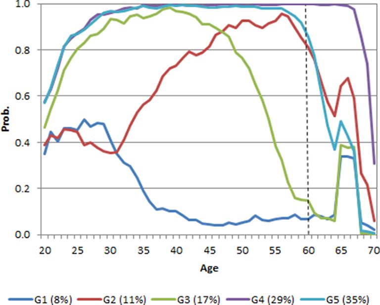
Checking the composition of the groups is a good way to validate also the trajectory analysis results. It is good practice to cross-tabulate the trajectory groups by the available background factors of the microsimulation. We have added an example which shows the labor market state or population state of earnings groups (k = 5) at age 60 in the simulated life-course (Figure 3). Depending on the available information of the microsimulation model, also other background factor could be cross-tabulated.

The labor market states (Table 2) confirm the earnings trajectory results. The high and stable wage earnings (employment) group G4 (29%) consists of people who are mainly (89.9%) in active labor market states. The weak attachment group G1 (8%) consists of individuals who had a disability or inactive status at the time. Also the share of deceased (15.5%) is higher in this group than in the other groups, which is quite natural. Another weak attachment group is G3 (17%), where the share of disabled and inactive individuals is relatively high compared to the other groups.

Table 2

Composition of earnings trajectories at age 60, per cent

	G1 (8%)	G2 (11%)	G3 (17%)	G4 (29%)	G5 (35%)	Total
Active first year	0.8	2.3	2.3	0.5	3.4	2.1
Active second year	0.4	0.6	0.7	0.3	0.9	0.6
Active (working)	2.3	51.1	1.2	89.9	54.2	50.6
Unemployed or in education	1.5	9.7	6.2	1.6	10.4	6.5
Sickness benefits	.	1.1	0.4	.	2.5	1.1
Partial disability pension and active	.	1.4	0.2	2.3	0.4	1
Partial disability pension and non-active	0.8	1.1	0.9	.	0.7	0.6
Full disability pension	23.4	2.8	26.9	0.5	2.9	7.9
Full disability pension second year	1.1	1.4	3.4	.	2	1.6
Old-age pension	.	.	0.5	0.1	0.7	0.4
Only national disability pension	15.5	.	.	.	.	1.2
Out of labor markets I	18.9	1.4	17.2	0.3	1.8	5.3
Out of labor markets II	14.3	.	2.5	.	0.8	1.9
Inactive	5.7	18.8	30.8	1.5	15.5	13.8
Deceased	15.5	8.2	6.9	2.8	3.8	5.5
Total	100	100	100	100	100	100

3.2. Education trajectories: class outcome

In this second example we continue to study the young cohort born in 1995 and illustrate a simulated life-course in terms of education level. This cohort finishes compulsory education at age 16 (in 2011). The subsequent education dynamics is simulated in the education module of the ELSI model.

The example shows a trajectory analysis with class-level outcome data. The distribution of the levels of education skewed to left (low education), therefore the outcome is modeled using the zero-inflated Poisson model. Yearly individual education information records the highest level of education. In practice, each individual level of education either remains unchanged or rises during the course of the simulation. Individuals enter the model at age 18 when 99% are at the basic education level. The ELSI model includes four levels of education: 0 = basic education (ISCED 0–3), 1 = secondary education (ISCED 4), 2 = lower academic degree (ISCED 5, 5B) and 3 = higher academic degree (ISCED 5A, 6).

The BIC score (Table 1) indicates that a six-group solution yields the best fit for the education outcome, but we also present the four-group and five-group solutions. Figure 4 shows that with the six-group solution, the smallest group comprises no more than 2% of the population.

The trajectory means clearly show how education dynamics play out in practice. For example, education increases sharply until around age 30, and then is virtually stagnant at age 40. In the four-group solution, the results are dominated by the final education level. The four-group and five-group solutions show adult and further education in action, with 6–7% of the cohort still on an upward education trajectory at later ages (k = 5: 6%, k = 6: 7%).

Overall, we have observed that 20% have a low education, 40% complete secondary education, 21% complete a lower university degree and 15% a higher university degree.

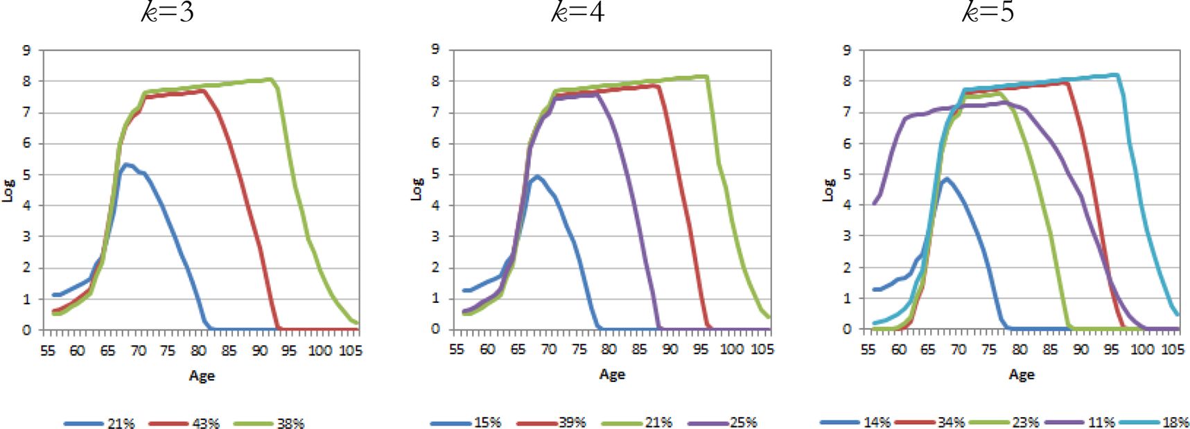
3.3. Pension trajectories: continuous outcome

The cohort in this third example was born in 1960. For this cohort, earnings, labor market state, accrued pensions and disability pension data are covered up to age 52 (in 2012). Thereafter, pension stock and new pensions are simulated in the ELSI model’s earnings-related pension module.

The example shows a trajectory analysis with continuous normal data. The outcome variable is earnings-related pension (log euros/month), excluding survivor’s pensions, expressed in nominal value. If an individual is not retired (not yet retired or deceased) the outcome value is zero, otherwise the individual is retired and receives a pension (Figure 5). The level of pension is determined by current pension rules for different types of pension benefit, such as disability pensions, partial old-age pensions and old-age pensions.

Figure 5

Download asset Open asset

Pension levels are affected by two factors. First, the most important factor that affects all retirees is indexation: earnings-related pensions are index-linked to prices (80%) and wages (20%). Second, some individuals continue to work while drawing their pension, which accrues additional pension benefits.

The BIC score (Table 1) indicates that the five-group solution yields the best fit for the pension outcome, but we also present the solutions for three-group and four-group solutions.

Trajectory analysis reveals several substantive issues. First, pensions increase as the cohort ages and approaches minimum retirement age at 64 years and 5 months (persons born in 1960 can retire flexibly between ages 64 years 5 months and 69 years). Pensions taken earlier are for the most part either disability pensions or partial old-age pensions. Second, the trajectories are affected by mortality as all trajectory means go to zero with the death of individuals in the group. For instance, one group (k = 5: 14%) dies early and its pension level remains low. This group, along with (k = 5: 11%), enters disability pensions at a higher rate than other groups. In addition, some groups have a higher life expectancy. The group with the highest life expectancy (k = 5: 18%) also has the highest pensions. Third, there is some indication of segregation among pensioners here.

It is also worth noting that pension indexation rules increase pensions in those sub-groups where life expectancy is high. Finally, an increase in the number of groups leads to the emergence of some interesting sub-groups. The early transition to disability pension is evident in the five-group solution (k = 5: 11%).

4. Conclusion

We have applied finite mixture modeling to longitudinal data in the context of dynamic microsimulation. It is useful in visualizing dynamic microsimulation results because it demonstrates, within a formal statistical structure, population heterogeneity in simulated datasets. Furthermore, the sub-groups identified in the analysis may reveal model misspecifications if such issues are present.

Our first goal was to illustrate the results of dynamic microsimulation, which are often presented as statistical moments or other distribution measures for a given population. Statistical moments presented on the basis of ex ante classification rules (e.g. gender, level of education, occupation or region) are a common way of reporting results for specific population sub-groups. We have shown how trajectory analysis can be applied as a data-driven method for illustrating longitudinal results in a novel way. These two ways of presenting results are mutually complementary.

Our second goal was to test the individual-level or object-level outcomes of dynamic microsimulation. Testing should be understood here by locating groups with unwanted or otherwise peculiar outcomes. Microsimulation easily yields biases and model misspecification. Microsimulation practitioners apply various techniques to calibrate models and to locate misspecification. Trajectory analysis could also be a useful tool in testing simulation model assumptions, as model misspecification may be revealed in developmental trajectories. Trajectory analysis together with other testing methods can improve microsimulation model reliability, especially in connection with large-scale revisions of model parameters.

There are some limitations with the proposed technique. First, it takes some effort to analyze all the cohorts included in the microsimulation model. It might be advisable to focus on some key cohorts if the simulation model assumes similar parameters across cohorts. Second, given the computational requirements of the EM algorithm, it is apparent that extremely large data sets (hundreds of thousands of individuals) should be avoided. A fraction or sample of the simulated data set usually reveals the underlying sub-populations with sufficient reliability. Third, it is necessary to mention conditional independence, even though this is not a serious drawback in a microsimulation context. Finally, basically trajectory analysis cannot handle nonlinear models. The group-specific regression model needs to be linear in parameters. However, reasonable approximations can often be provided by low-degree polynomial models.

Trajectory analysis is also a highly flexible method. In our case we performed the analysis for one outcome at the time, but the technique and software is in place to model several outcomes at the same time. This is called multi-trajectory modeling, which identifies groups of individuals or objects that follow similar trajectories across multiple outcomes. For example, it would be possible to analyze income, education and labor market status simultaneously. This would yield a slightly different probability for belonging to a specific group. Another possibility would be to add time-dependent (e.g. earnings) or time-stable (e.g. gender, year of birth or nationality) covariates alongside age or time polynomial. This would be a case of multinomial logistic regression within a population sub-group, and the result would consist of risk factors influencing group membership.

Footnotes

1.

SAS package PROC TRAJ counts BIC and AIC routinely.There are other information criteria, like cross-validation available, if the number of sub-groups is critical for the microsimulation practitioner (see Nielsen et al., 2014).

2.

SAS and STATA (see Jones and Nagin, 2013) trajectory analysis package can be downloaded from the website: https://www.andrew.cmu.edu/user/bjones/. R package for trajectory analysis is Flexmix (see Leisch, 2004).

Appendix

A.1 An example SAS PROC TRAJ-code.

Earnings trajectories: Five-group solution

Males born 1995
Simulated yearly wage earnings 2015–2080
Binary outcome 1 = some wage, 0 = no wage
WMALE_1995 is the individual level data set with yearly observations on binary wage (bwage) and age (age).

The PROC TRAJ produces four output datasets. OP includes the group mean estimates and confidence intervals (95%). OS includes the mixture components (sizes of the sub-groups). OF includes individual-level information on group posterior probabilities and group assignment. This is an important data set where we can merge any other relevant background information. Finally, OE includes the regression model coefficients and information criteria (AIC and BIC). ITDETAIL statement shows the progression of maximum likelihood estimation in the SAS log window.

Algorithm 1

PROC TRAJ.

1: PROC TRAJ DATA=WMALE_1995 OUTPLOT=OP OUTSTAT=OS OUT=OF OUTEST=OE ITDETAIL;

2: ID idno;

3: VAR bwage2015-bwage2080;

4: INDEP age2015-age2080;

5: MODEL logit;

6: NGROUPS 5;

7: ORDER 3 3 3 3 3;

8: RUN;

The actual model is specified with VAR, INDEP, MODEL and ORDER statements. The MODEL logit states that we analyze binary outcomes. Other possibilities are censored normal outcome (cnorm) and zero-inflated Poisson outcome (zip). NGROUP states the number of sub-groups. ID states the number of individuals. ODRER defines the number of mixture components (=NGROUPS) and respective degree of age-polynomial. Each sub-group can have different degrees of age-polynomial.

Algorithm 2

TRAJPLOT-macro.

1: %TRAJPLOT(OP,OS,,);

2: RUN;

3: DATA WMALE_1995; MERGE WMALE_1995 OF (KEEP=idno group); BY idno;

4: RUN;

The TRAJPLOT macro statement invokes the result plot, which by default plots the trajectory means and their estimates. Finally, individual level results are collected and merged with microsimulation output dataset.

A.2 Summary of Estimated Model: Outcomes, Groups, Parameter Estimates and their Standard Errors.

Outcome	Groups	${\hat{β}}_{0}$	$S E ({\hat{β}}_{0})$	${\hat{β}}_{1}$	$S E ({\hat{β}}_{1})$	${\hat{β}}_{2}$	$S E ({\hat{β}}_{2})$	${\hat{β}}_{3}$	$S E ({\hat{β}}_{3})$
Earnings	1	−0.60816	0.93616	0.17156	0.07229	−0.00845	0.00173	0.00008	0.00001
Earnings	2	10.77241	0.7512	−1.05243	0.05715	0.03048	0.00135	−0.00026	0.00001
Earnings	4	−24.0041	0.69707	1.88334	0.05421	−0.04084	0.00128	0.00026	0.00001
Earnings	5	2.89272	0.93197	−0.55508	0.08212	0.02763	0.00225	−0.00029	0.00002
Education	1	150.7634	13.69866	−23.324	1.03504	0.60943	0.01352	−0.00442	0.00018
Education	2	−38.2479	1.84202	1.95442	0.10906	−0.03343	0.00214	0.00019	0.00001
Education	3	−1.40435	0.08235	0.09431	0.00638	−0.00206	0.00016	0.00001	0.00000
Education	4	−3.82746	0.09413	0.27969	0.00712	−0.00568	0.00017	0.00004	0.00000
Education	5	−6.14041	0.09384	0.46159	0.00701	−0.00958	0.00017	0.00006	0.00000
Education	6	−34.1529	1.02762	2.02103	0.06446	−0.03841	0.00133	0.00024	0.00001
Pension	1	1352.226	1.29912	−66.1983	0.03537	1.07053	0.0006	−0.00572	0.00001
Pension	2	−220.279	3.93005	5.68868	0.15254	−0.03308	0.00196	−0.00003	0.00001
Pension	3	−464.879	3.77328	14.13735	0.14801	−0.12224	0.00197	0.00024	0.00001
Pension	4	27.60321	4.88433	−1.86771	0.19721	0.03987	0.00262	−0.00025	0.00001
Pension	5	−127.459	2.91581	3.18956	0.10992	−0.01691	0.00136	−0.00002	0.00001

References

1
Latent class growth modelling: a tutorial
(2009)
Tutorials in Quantitative Methods for Psychology 5:11–24.
https://doi.org/10.20982/tqmp.05.1.p011
- Google Scholar
2
Advances in mixture models
1. D Böhning
2. W Seidel
3. M Alfó
4. B Garel
5. V Patilea
6. G Walther
(2007)
Computational Statistics & Data Analysis 51:5205–5210.
https://doi.org/10.1016/j.csda.2006.10.025
- Google Scholar
3
Applications of microsimulation modelling
1. G Dekkers
2. K Van den Bosch
(2016)
Prospective microsimulation of pensions in European Member States, Applications of microsimulation modelling.
- Google Scholar
4
Maximum likelihood estimation for incomplete data via the EM algorithm
(1977)
Journal of the Royal Statistical Society B 39:1–38.
- Google Scholar
5
Relationship satisfaction trajectories across the transition to parenthood among low-risk parents
1. BP Don
2. KD Mickelson
(2014)
Journal of Marriage and Family 76:677–692.
https://doi.org/10.1111/jomf.12111
- Google Scholar
6
SESIM III - A Swedish dynamic micro simulation model
(2012)
SESIM III - A Swedish dynamic micro simulation model.
- Google Scholar
7
Model 1: MOSART (Dynamic Cross-Sectional Microsimulation Model)
1. D Fredriksen
2. N Stølen
(2007)
In: Anil Gupta, Ann Harding, editors. Modelling Our Future: Population Ageing, Health and Aged Care (International Symposia in Economic Theory and Econometrics, Volume 16). Emerald Group Publishing Limited. pp. 433–437.
- Google Scholar
8
FlexMix: an R package for finite mixture modelling
1. B Grun
2. F Leisch
(2007)
Faculty of Commerce – Papers.
- Google Scholar
9
Review of three latent class cluster analysis packages: latent GOLD, poLCA, and MCLUST
(2009)
The American Statistician 63:81–91.
https://doi.org/10.1198/tast.2009.0016
- Google Scholar
10
Trajectories of multimorbidity and impacts on successful aging
1. H-C Hsu
(2015)
Experimental Gerontology 66:32–38.
https://doi.org/10.1016/j.exger.2015.04.005
- Google Scholar
11
Women’s employment patterns during early parenthood: a group-based trajectory analysis
1. K Hynes
2. M Clarkberg
(2005)
Journal of Marriage and Family 67:222–239.
https://doi.org/10.1111/j.0022-2445.2005.00017.x
- Google Scholar
12
Advances in group-based trajectory modeling and an SAS procedure for estimating them
1. BL Jones
2. DS Nagin
(2007)
Sociological Methods & Research 35:542–571.
https://doi.org/10.1177/0049124106292364
- Google Scholar
13
A note on a STATA plugin for estimating group-based trajectory models
1. BL Jones
2. DS Nagin
(2013)
Sociological Methods & Research 42:608–613.
https://doi.org/10.1177/0049124113503141
- Google Scholar
14
A SAS procedure based on mixture models for estimating developmental trajectories
(2001)
Sociological Methods & Research 29:374–393.
https://doi.org/10.1177/0049124101029003005
- Google Scholar
15
Simulating an Ageing Population: A microsimulation approach applied to Sweden
1. A Klevmarken
2. B Lindgren
(editors) (2008)
Bingley: Emerald Group Publishing Ltd.
- Google Scholar
16
Trajectories based on Postcomprehensive and higher education: their correlates and antecedents
(2008)
Journal of Social Issues 64:59–76.
https://doi.org/10.1111/j.1540-4560.2008.00548.x
- Google Scholar
17
FlexMix: A General Framework for Finite Mixture Models and Latent Class Regression in R
1. F Leisch
(2004)
Journal of Statistical Software 11:1–18.
https://doi.org/10.18637/jss.v011.i08
- Google Scholar
18
A survey of dynamic microsimulation models: uses, model structure and methodology
1. J Li
2. C O’Donoghue
(2013)
International Journal of Microsimulation 6:3–55.
- Google Scholar
19
Handbook of Microsimulation Modelling. Contributions to economic analysis
(2014)
Dynamic models, Handbook of Microsimulation Modelling. Contributions to economic analysis, Emerald.
- Google Scholar
20
Statistical Analysis with Missing Data
1. R Little
2. D Rubin
(1987)
New York: John Wiley & Sons.
- Google Scholar
21
The differential impacts of markets for technology on the value of technological resources: an application of group-based trajectory models
1. D Mani
2. A Nandkumar
(2016)
Strategic Management Journal 37:192–205.
https://doi.org/10.1002/smj.2457
- Google Scholar
22
Finite Mixture Models
1. G McLachlan
2. D Peel
(2000)
New York: John Wiley and Sons Inc.
- Google Scholar
23
MPlus Statistical Analysis With Latent Variables, User’s Guide
1. L Muthén
2. B Muthén
(2010)
MPlus Statistical Analysis With Latent Variables, User’s Guide, Los Angeles, CA.
- Google Scholar
24
Analyzing developmental trajectories: a semiparametric, group-based approach
1. DS Nagin
(1999)
Psychological Methods 4:139–157.
https://doi.org/10.1037/1082-989X.4.2.139
- Google Scholar
25
Group-Based Modeling of Development
1. D Nagin
(2005)
Cambridge, MA: Harvard University Press.
- Google Scholar
26
Group-Based trajectory modeling and criminal career research
1. DS Nagin
(2016)
Journal of Research in Crime and Delinquency 53:356–371.
https://doi.org/10.1177/0022427815611710
- Google Scholar
27
The Wiley Handbook of Developmental Psychopathology
(2017)
Developmental Trajectories of Psychopathology. An Overview of Approaches and Applications, The Wiley Handbook of Developmental Psychopathology, John Wiley & Sons Ltd.
- Google Scholar
28
Group-Based criminal trajectory analysis using cross-validation criteria
1. JD Nielsen
2. JS Rosenthal
3. Y Sun
4. DM Day
5. I Bevc
6. T Duchesne
(2014)
Communications in Statistics - Theory and Methods 43:4337–4356.
https://doi.org/10.1080/03610926.2012.719986
- Google Scholar
29
Group-Based multi-trajectory modelling
1. D Nagin
2. B Jones
3. L Passos
4. R Tremblay
(2016)
Statistical Methods in Medical Research pp. 1–9.
- Google Scholar
30
Group-Based trajectory modeling (nearly) two decades later
1. DS Nagin
2. CL Odgers
(2010)
Journal of Quantitative Criminology 26:445–453.
https://doi.org/10.1007/s10940-010-9113-7
- Google Scholar
31
A trajectory analysis of body mass index for Finnish children
1. T Nummi
2. T Hakanen
3. L Lipiäinen
4. U Harjunmaa
5. MK Salo
6. M-T Saha
7. N Vuorela
(2014)
Journal of Applied Statistics 41:1422–1435.
https://doi.org/10.1080/02664763.2013.872232
- Google Scholar
32
Trajectories of a set of ten functional somatic symptoms from adolescence to middle age
(2017a)
Archives of Public Health 75:11.
https://doi.org/10.1186/s13690-017-0178-8
- Google Scholar
33
New Advances in Statistics and Data Science
(2017)
Statistical Analysis of Labor Market Integration: A Mixture Regression Approach, New Advances in Statistics and Data Science, ICSA Book Series in Statistics, Springer.
- Google Scholar
34
Job Contract at Birth of the First Child as a Predictor of Women’s Labor Market Attachment: Trajectory Analyses over 11 Years
(2015)
Nordic Journal of Working Life Studies 5:9–30.
https://doi.org/10.19154/njwls.v5i1.4763
- Google Scholar
35
Eläketurvakeskuksen ELSI-mikrosimulointimallin laajennus Kelan eläkkeisiin ja verotukseen
1. H Sihvonen
(2015)
Eläketurvakeskuksen ELSI-mikrosimulointimallin laajennus Kelan eläkkeisiin ja verotukseen, Finnish Centre for Pensions Working papers 03/2015.
- Google Scholar
36
Microsimulating Finnish earnings-related pensions
(2014)
Finnish Centre for Pensions Working Papers 02/2014.
- Google Scholar
37
Distributional effects of forthcoming Finnish pension reform – a dynamic Microsimulation approach
(2015)
International Journal of Microsimulation 8:75–98.
- Google Scholar
38
Statutory pensions in Finland – long-term projections 2016
(2017)
Statutory pensions in Finland – long-term projections 2016, Finnish Centre for Pensions Reports 02/2017.
- Google Scholar
39
Statistical analysis of finite mixture distributions
(1985)
Great Britain: John Wiley & Sons.
- Google Scholar
40
The effects of incarceration on longitudinal trajectories of employment: a follow-up in high-risk youth from ages 23 to 32
(2016)
Crime & Delinquency 62:107–140.
- Google Scholar
41
Dynamic Microsimulation Models: A Review and Some Lessons for SAGE
1. A Zaidi
2. K Rake
(2001)
The London School of Economics.
- Google Scholar

Article and author information

Author details

Janne Salonen

Finnish Centre for Pensions, Helsinki, Finland

For correspondence
janne.salonen@etk.fi

Competing interests
No competing interests reported

"This ORCID iD identifies the author of this article:" 0000-0002-0595-6226
Heikki Tikanmäki

Finnish Centre for Pensions, Helsinki, Finland

For correspondence
heikki.tikanmaki@etk.fi

Competing interests
No competing interests reported
Tapio Nummi

University of Tampere, Tampere, Finland

Competing interests
No competing interests reported

Funding

No specific funding for this article is reported.

Acknowledgements

The authors wish to thank Statistics Finland for providing material for this study and two anonymous referees as well as chief editor Matteo Richiardi for their many thoughtful comments that greatly improved this paper.

Publication history

Version of Record published: August 31, 2019 (version 1)

Copyright

This article is distributed under the terms of the Creative Commons Attribution License, which permits unrestricted use and redistribution provided that the original author and source are credited.

Download links

A two-part list of links to download the article, or parts of the article, in various formats.

Downloads (link to download the article as PDF)

Article PDF

Download citations (links to download the citations from this article in formats compatible with various reference manager tools)

BibTeX
RIS

Open citations (links to open the citations from this article in various online reference manager services)

Mendeley

Structure of the ELSI microsimulation model

BIC scores and number of sub-groups k

Earnings trajectories

Earnings trajectories, k=5

Education trajectories

Composition of earnings trajectories at age 60, per cent

Pension trajectories

PROC TRAJ.

TRAJPLOT-macro.

Author details

Janne Salonen

For correspondence

Competing interests

Heikki Tikanmäki

For correspondence

Competing interests

Tapio Nummi

Competing interests

Downloads (link to download the article as PDF)

Download citations (links to download the citations from this article in formats compatible with various reference manager tools)

Open citations (links to open the citations from this article in various online reference manager services)

Categories and tags