Developing a microsimulation model for farm forestry planting decisions
- Teagasc, Rural Economy & Development Programme, Ireland
- National University of Ireland, Ireland
Abstract
There is increasing pressure in Europe to convert land from agriculture to forestry which would enable the sequestration of additional carbon, thereby mitigating agricultural greenhouse gas production. However, there is little or no information available on the drivers of the land use change decision from agriculture to forestry at individual farm level, which is complicated by the inter-temporal nature of the decision. This paper describes a static microsimulation approach which provides a better understanding of the life-cycle relativity of forestry and agricultural incomes, using Ireland as a case-study. The microsimulation methodology allows for the generation of actual and counterfactual forest and agricultural income streams and for other attributes of utility such as long-term wealth and leisure, for the first time. These attributes are then modelled using purpose built forest models and farm microdata from a 30 year longitudinal dataset. The results show the importance of financial drivers but additionally show that wealth and leisure are also important factors in this inter-temporal land use change decision. By facilitating the examination of the distribution of farms across the farming population, the use of a static microsimulation approach allows us to make a considerable contribution to the literature in relation to the underlying drivers of farm afforestation behaviour. In the broader context of Climate Smart Agriculture and the Grand Challenges facing the intensification of agricultural production, these findings have implications for policies that seek to optimize natural resource use.
1. Introduction
There is increasing pressure in Europe to convert land from agriculture to forestry which would enable the sequestration of additional carbon, thereby mitigating agricultural greenhouse gas production.1 The recognition of the multiple values of forests has led to international efforts to increase the planting of new forests (afforestation). However, despite the provision of economic incentives, afforestation targets across Europe are not being met (European Commission, 2013).2 This policy failure has consequences downstream in the value chain in for timber processing, for increasing demand for wood fibre and for the potential of forests to sequester carbon and mitigate greenhouse gas emissions. In this paper, we develop a microsimulation model to help to understand the drivers of forest planting behaviour
This paper develops a microsimulation based framework looking at the drivers of decisions in relation to afforestation (new planting). The literature suggests that a number of factors affect the afforestation decision. In a meta-analysis (Beach et al., 2005) assessed the primary factors driving decision-making among landowners considering afforestation: owner characteristics, plot/resource conditions, factors that affect the forest investment decision and market drivers (costs and returns from forestry and alternative enterprises). Edwards and Guyer (1992) reported that the principal constraints to planting in the UK include lack of land, duration of the commitment and the inability of the annual subsidy payments to compete with agricultural returns. Van Gossum et al. (2012) and Moons and Rousseau (2007) suggest that Flemish forest subsidies are not high enough and the absence of financial benefits for farmers was one of the main reasons for the limited uptake by farmers in the Netherlands (Van Gossum et al., 2010).
With the growing importance of natural resource and environmental issues in policy spheres, the microsimulation literature has been developing in natural resource spheres such as agriculture, environment and land use (Richardson et al., 2014; Hynes and O’Donoghue, 2014; O’Donoghue, 2017; Ryan et al., 2014). In developing a microsimulation model with the aim of simulating the drivers of afforestation behavior on farms, this paper charts the development of one of the first forestry based microsimulation models.
While our interest in this study is on drivers of behaviour, we do not develop a behavioural simulation model, but one that is static in nature, where we develop a static microsimulation framework which takes a population distribution and simulates ‘day-after policy’ changes on farms. Thus we develop a model initially with a focus on drivers of forestry planting behaviour. It is therefore a forestry parallel to the microsimulation literature that looks at tax and social policy. In understanding pressures on behavior, this analysis develops static-based measures akin to the use of replacement rates (O’Donoghue, 2011) and marginal effective tax rates (Immervoll, 2005). In doing this, we model the impact on income and public transfers and other issues such as land value and hours worked as a result of converting agricultural land to forestry. We consider in particular the differential implications of planting across the distribution of farms, noting significant heterogeneity amongst farms. Further light could also be shed on the levers driving the land use change by specifically comparing the farm incomes and incentives for those farms that have planted in the past against the farm incomes and incentives that applied to farms without forests.
We select Ireland as a case study as it is the country within Europe that saw the most rapid increase in afforestation following the introduction of financial incentives for the afforestation of agricultural land. The period 1985 to 1995 saw a rapid increase in annual planting by farmers from just over 5,000 ha to almost 24,000 ha. In recent years however, the decline in afforestation rates has equally been most pronounced in Ireland relative to other European countries as the planting rate has fallen off to just under 5,000 ha in recent years(Forest Service, 2018), despite substantial increases in subsidy payments. Studies that specifically examine farmer afforestation in Ireland have found that there is a preference not to plant land that is profitable in agriculture (Frawley and Leavy, 2001; O’Leary et al., 2000; McDonagh et al., 2010; Ní Dhubháin and Gardiner, 1994; Duesberg et al., 2013; Duesberg et al., 2014) and a strong preference for the utility or value that farmers derive from the farming lifestyle. Increasingly, the loss of flexibility of land use as a result of the permanence of forestry is seen as a barrier to afforestation (McDonagh et al., 2010; Duesberg et al., 2014; Duesberg et al., 2013).
This paper develops a model to simulate financial and lifestyle drivers of the forestry planting decision. The analysis utilises farm micro data together with bio-economic forestry models and forest subsidy models to estimate the return from an alternative agricultural land use. An examination of the combination of these data and factors has not previously been undertaken in the forestry literature and is facilitated here by the use of microsimulation modelling, which abstracts from reality to better understand complexity (O’Donoghue, 2014). In Section 2 the factors influencing a long-term participation decision such as forestry are investigated in order to develop a theoretical framework. Section 3 describes the generation of the variables used in the models and Section 4 presents the results. We finish with discussion and conclusions.
2. Theoretical framework
In determining the nature of the microsimulation model required to simulate the drivers of afforestation behaviour, we firstly examine the theoretical framework required to compare the incentives of alternative land uses. The literature that addresses the land use change from agriculture to forestry (or farm afforestation) is actually quite limited as the vast majority of studies in relation to the economics of forestry focus on deforestation or management decisions in pre-existing forests.
As the return from forestry is quite long term with potentially a 40–50 year gap between planting and harvesting for coniferous trees (and longer (up to 150 years) for deciduous trees), afforestation is a long-term investment. Even with the long term planning horizon, afforestation is an unusual land use change as it is a permanent change in many countries (there is a legal requirement to re-plant the land after timber harvesting (Ryan et al., 2016). Conversely, the alternative land use, agriculture, has a relatively short time horizon with a one to three year cycle for agricultural produce. Thus the land use change incurs an inter-temporal annual opportunity cost foregone from existing farm enterprises such as dairy, cattle rearing, sheep or tillage enterprises. In comparing alternative land uses over a long period of time, we will need to model alternative income streams over a long time period and the consequential differences in the net present value of income.
The literature that deals with agricultural opportunity costs in the context of farm afforestation is also limited and focuses largely on the calculation of the opportunity cost of carbon sequestration through afforestation at an aggregate level (see Moulton and Richards, 1990; O’Leary et al., 2000). Due to the policy complexity of comparing agricultural and forestry income streams over time, studies in this area are based largely on average opportunity costs across farm systems. O’Connor and Kearney (1993), McCarthy et al. (2003) and Ryan et al. (2014), use average values to highlight the importance of the loss of agricultural subsidies when land is planted. In calculating the net return from farm afforestation, Dudek and LeBlanc (1990) use average agricultural opportunity costs and Breen et al. (2010) use average farm management data (Teagasc, various years) to calculate the opportunity cost of the superseded agricultural enterprise, while Upton et al. (2013) compare average life-cycle agricultural and forest incomes. Herbohn et al. (2009) go further and use actual farm input data to calculate the agricultural opportunity cost of planting on individual farms. However, in reality there is a large degree of income heterogeneity at individual farm level, yet to our knowledge, there are no studies that examine the distribution of farms in quantifying the life-cycle financial drivers that influence planting behaviour.
As farm afforestation is essentially a permanent land-use change which imposes loss of flexibility in relation to land use (as there is a legal obligation to retain land under forest once planted), we expect that planting could negatively impact on the long-term wealth of farmers, as planted land is no longer available for agriculture for current or future generations. Therefore in addition to changes in the net present value of income, we need also to consider changes in farm wealth, by examining whether there is a difference in farmers’ perception of the value of their land before and after planting.
Traditional economic theory suggests that individuals make decisions based on the expected change in their level of ‘well-being’, where the term used for well-being or welfare is utility (Edwards-Jones, 2006). Given that utility is a difficult concept to measure, economists have often made the simplifying assumption that money can act as a substitute for utility. This has led to the situation observed in many agricultural economic models in which farmers act to maximise profitability in all circumstances (Edwards-Jones, 2006). However, the Random Utility Maximisation (RUM) and Discrete Choice methodologies employed by McFadden, 1973 and Ben-Akiva and Lerman (1985) incorporate the value of leisure time as a component of utility.
Labour requirements also differ between agricultural and forest land use. Relatively little labour is required for forest management on a day to day basis, whereas for an animal based agricultural system, there are regular day-to-day labour requirements, e.g. feeding and maintaining the animals and grassland management. Thus we expect that farmers who plant land have reduced working hours with a consequent increase in potential leisure time period. This may act as an incentive for farmers who are motivated by life-style and may be willing to make a trade-off between income and leisure (Ryan et al., 2015).
Previous studies have highlighted the importance of the relative potential incomes from agriculture and forestry. However, the impact of planting on annual income is less clear because the sources of income are so different. Agriculture and forestry are highly regulated and subsidised businesses, given the public good nature of many of the outputs. Income is thus derived from both market and public sources. Agricultural income includes annual market income and agricultural policy subsidies, which are tied either to production in the case of coupled payments, or land in the case of decoupled payments.3 As planting land results in a reduction in the agricultural land area, agricultural subsidy payments may be reduced on planting. The opportunity costs of planting arising from the loss of agricultural market and subsidy income are intertemporal in nature as they are essentially incurred for each year of the forest rotation.
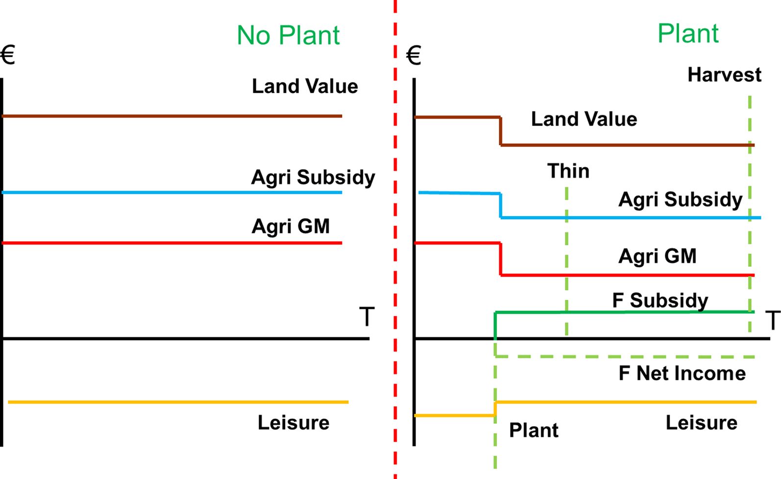
Income from forestry is net of up-front planting costs, regular maintenance and management costs,with periodic thinning costs. Income may arise from periodic thinnings with harvesting income arising at the end of the forest rotation. Afforestation income streams also include considerable policy subsidies. Thus, losing land from agriculture to forestry, in a straight land use change, sees a reduction in both agricultural market incomes and subsidies and ‘lumpy increases in forestry market incomes and subsidies. The time-lines of the market and subsidy income, along with the wealth and leisure components of the farm afforestation decision are important in developing the inter-temporal framework and are presented graphically in Figure 1.

Timelines of financial, policy and leisure components of the utility associated with the land use change from agriculture to forestry
Source: Ryan et al. (2015).
Note: Agri GM = Agricultural Gross Margin = Agri Market Income – Agri Costs.
Apart from the high-level income, wealth and leisure differences between agriculture and forestry, there is also significant micro-unit variability as farms can vary by soil type and agronomic characteristics (which influence productivity), farm system (which influences incomes and costs) and individual farmer characteristics and skills (which influence efficiency and investment decisions). Thus we expect the drivers of the planting decision to vary considerably across farm types.
In summary, the inter-temporal modelling of the differential life-cycles of the agricultural and forest income cycle factors addressed in the literature should provide a better understanding of the direct and indirect opportunity costs faced by individual farmers in considering forestry. However, due to the dearth of farm forestry micro-data, previous studies have been undertaken either using aggregate data or sectoral averages, yet these do not consider the differential farm and farmer characteristics and environmental conditions that apply at individual farm level. Thus an analytical, microsimulation based approach that provides information on the economic drivers of planting behaviour - across the distribution of farms - is appropriate to model alternative land use decisions and assess the impact of financial and lifestyle drivers.
3. Methodology and data
This study develops a model that simulates at a micro-level, the market, environmental, policy and leisure drivers of forestry planting, in an inter-temporal framework. Here we describe the methodology used to develop a farm-forest microsimulation model which allows us to compare income streams over time between the alternative land uses of agriculture and forestry.
3.1. Farm forestry microsimulation model
The use of a microsimulation approach here allows for the consideration of two dimensions of complexity, the policy/market and the distributional characteristics, namely a static microsimulation model (Li et al., 2014). Static models take individual characteristics and behaviours as exogenous and are commonly referred to as models that estimate the ‘day after’ impact of a policy reform, ignoring the behavioural response impact due to the policy. While it would be interesting to model the response to policy changes on the probability of afforestation, given the complexity of the decision-making process, a necessary pre-condition is to first understand the drivers of economic (annual income and overall wealth) and working hours/leisure of planting behavior.
To understand the economic drivers of forest planting behaviour, one needs to understand the full range of factors that influence the opportunity cost of planting, namely (a) the potential forest market and subsidy income streams arising from afforestation, given the specific soil/productivity conditions for individual farms; (b) the annual agricultural market and subsidy income foregone for each year of the forest rotation (depending on soil/productivity conditions of individual farms); and the impact of planting on changes in long-term land value (wealth) and hours worked (leisure).
In this paper, we want to examine the impact of planting one additional hectare of forest on overall farm income, land value and leisure. Thus we simulate the marginal impact of a planting decision on the factors described above. This is similar methodologically to how the marginal effective tax rate (METR) is calculated in the household microsimulation literature, which examines the degree to which an increase in income of one euro would be ‘taxed away’ from a combination of all instruments, thus influencing household behaviour (Immervoll, 2004).
The simulation approach undertaken here, drawing upon the method used in Immervoll (ibid) allows for the calculation of the marginal effect of planting on all income sources associated with both the existing land use, agriculture and the alternative land use forestry. This paper follows this methodology and utilises micro-data from a static population of farms to examine the impact of planting on agricultural income and hours worked.
In order to model the distribution of farmers in Ireland, this analysis utilizes a micro dataset of potential farm forests in order to compare the distribution of incentives for farms that have already planted (has forest) versus farms that haven’t planted (no forest). This is undertaken by simulating (a) counterfactual forest income observations for farms that didn’t plant and (b) counterfactual agricultural incomes for farms that planted land.
The use of microsimulation models has grown in recent years in agriculture and natural resource policy. While static microsimulation models can be regarded as being ‘simpler’ microsimulation models, ignoring behavioural, temporal or spatial effects, simulations can still be complex as the modelling process tries to represent the heterogeneous patterns of interacting population structures and policy complexity. To our knowledge, this is the first example of a forestry-focused static microsimulation model in the literature.
3.2. Methodological choices
Developing microsimulation models involves many methodological choices. A wide range of parameters have been identified throughout the literature, including:
type of microsimulation (what)
unit of analysis & variation (who) and
unit of measurement (how & how much).
The modelling options required for static microsimulation models are presented in the following sections, referring in particular to two bespoke forest models developed to model the forest policy environment in Ireland since the 1980s, namely the Teagasc Forest Subsidies (ForSubs) model developed by Ryan et al. (2014) and the Teagasc Forest Bio-economic Systems (ForBES) model developed by Ryan et al. (2016), which in combination, generate life-cycle forest incomes by modelling forest subsidies and the biological system associated with tree growth, volume production and timber values for a range of species with different environmental conditions and management practices.
3.3. Unit and period of analysis
The choice of the unit of analysis is a key decision of a model builder. Two bespoke forestry models are utilised to understand the comparative advantage of forestry versus agricultural land use, so the common unit of analysis is land and in particular, the farm. Thus the comparative analysis is conducted in relation to subsidies or incomes at the hectare (ha) level. The ForSubs model generates the forest subsidy relevant for the conversion of land from agriculture to forestry (on a per hectare basis), in a given year, while the ForBES model generates forest market income (also on a per hectare basis).
The next methodological choice is the period of analysis. This refers to the time period over which an analysis applies. The analyses described thus far relate to policies within a particular period. Most policy models focus on the current period and typically model work incentives (Immervoll, 2005). However analyses such as those considered in pensions or education financing are undertaken over longer life-cycle horizons (Falkingham et al., 1999). The conversion of agricultural land to forestry is such a life-cycle choice, thus the period of analysis extends over the full life cycle of a forest.
3.4. Analytical measures used
Fundamental to the analytical choice is the specific analytical measure used. The afforestation decision is essentially an investment decision as farmers ’invest’ their land in forestry. The analytical measures used to model the return on investment vary from nominal values to benefit-to-tax ratio (James and Villas, 2000; Thorburn et al., 2007) to Net Present Value (NPV) (Geanakoplos et al., 1998) to Internal Rate of Return (IRR), depending on the type of investment.
Within the field of agriculture, the primary focus is on quantifying the costs associated with a given level of production, quantifying the relative profit margin, the total cost and the opportunity costs of different production systems (Thorne and Fingleton, 2006). In the case of examining the land use change from agriculture to forestry, the analytical measures of return required are those which incorporate the inter-temporal nature of the decision, but also facilitate comparison between the opportunity cost of the annual (agricultural) income and multi-annual (forest) income.
A life-cycle framework is thus required to capture the implications of different afforestation and forest management choices. Discounted Cash Flow (DCF) is the most widely used methodology for determining the economic value of a forest or a parcel of bare land to be afforested (Hiley, 1954). The DCF methodology involves the calculation of the net present value4 (NPV), using the , 1849 formula. In recent years, the inclusion of non-market values in sustainable forest management (SFM) requires broader thinking and more complex models but the Faustmann formula remains appropriate for sustained yield plantation forests (Kant, 2003).
The choice of calculation methodology depends on whether the period of analysis reflects one rotation or an infinite number of rotations. The primary interest of this analysis is the comparison of annual returns from an agricultural enterprise against the returns from forestry over one rotation. Using NPV to generate the future value of the forest involves the projection of costs and incomes forward and then discounting these costs and incomes to the present day, at a target rate of interest (Hiley, 1954), thus equation 1 defines
where n is the number of years into the future (in this case the number of years of the forest rotation) that the income amount (I) will be received, or spent if the income amount is negative.
In the case of a forest, income and costs can accrue unevenly over the rotation, thus the net present value (NPV) of the whole income stream is the sum of the present values of the annual amounts in the income stream as presented in equation (3), (assuming a constant discount rate).
Both market and non-market income streams are included in NPV calculations as described in the next sections.
3.5. Generation of forest subsidies
The paramaterisation of annual changes in forest subsidy eligibility criteria, payment rates, forest species composition, and area limitations was undertaken by Ryan et al. (2014) in developing the Teagasc ForSubs model. The main factors which determine the rate of payment of forest subsidies are:
year of afforestation and area planted
eligibility for higher “farmer” rate of subsidy
LFA[5] status
species choice is largely governed by forest yield class (yc) which is a measure of the average volume production over the lifetime of a forest crop.
3.6. Generation of forest market income
As there is little or no microsimulation literature that addresses afforestation, this paper provides information on the forest growth and market parameters that are required to model farm forests, using the Teagasc ForBES model (Ryan et al., 2016), which estimates future timber volume production on the basis of specific agronomic and management factors, utilizing the forest yield models of Edwards and Christie (1981). Timber revenues are calculated by multiplying the timber volume by the relevant timber prices for given log size categories. All establishment, management and harvesting costs are subtracted from incomes to arrive at future net income flows.[6] These are then discounted to provide the economic return on a forest, given specific afforestation and management choices such as whether the forest is thinned or not[7]. In calculating forest market income in the context of a land use change from agriculture to forestry, the annual opportunity cost of the superseded agricultural enterprise should also be included.
ForBES incorporates outputs from ForSubs to generate total NPV annual forest (market and subsidy) income for each year of a forest rotation. However, it is only possible to make direct comparisons between the NPV return on two investments (in this case, land uses) if both land uses have the same life spans. Thus the NPV needs to be annualised so that it can be expressed on the same basis as annual agricultural returns. The AE value is calculated as follows:
In order to examine multi-annual forest life-cycle incomes, a discount factor is employed. Essentially, current (2015) input prices are examined and a decision is taken as to whether to adjust these forward for the life-cycle using a consumer price index (CPI), or whether to hold both costs and prices constant for the life-cycle. The NPV calculation then discounts this back to the present day value.
The discount rate chosen for the NPV calculations can significantly increase or decrease the returns from an afforestation project. There are essentially two components within the discount factor, one which accounts for time preferences and represents the return to money in the bank and the second which accounts for risk. The convention in Ireland is to use a real rate of 5% (Clinch, 1999), reflecting an interest rate of 3% and a risk premium of 2% for risk elements such as fire, wind-blow and market risk (Phillips et al., 2013). For a forest investment with the common pattern of incurring costs in the early years and not accruing profits until later, using a higher discount rate will reduce the NPV. The convention is to ignore any effects of possible inflation, as this cannot be predicted. Therefore, the return is regarded as a ‘real’ rate of return.
The ForBES and ForSubs models do not include a taxation component. The convention for forest valuation is to generate pre-tax values for agriculture and forestry as per the International Accounting Standard (IAS 41 – Agriculture) (EC, 2009).
3.7. Generation of agricultural income streams using farm survey micro data
The primary data source for this analysis is the Teagasc National Farm Survey (NFS) which is Ireland’s contribution to the EU Farm Accountancy Data Network (FADN). The NFS collects detailed information from a representative sample of farms in Ireland over the period 1985–2013 (inclusive) which contains farm and farmer characteristics of the farms that chose to afforest land over the period as well as those that did not choose to afforest land. The data are used to generate long-term agricultural cost and revenue streams for each of six agricultural systems (dairy, cattle rearing, cattle other, sheep, tillage and mixed livestock) on six soil types. The consumer price index (CPI) for 2013 is applied to all incomes to make them comparable.
Data were also utilised from a Teagasc NFS supplementary survey conducted in 2012, which collected additional attitudinal questions, including whether farmers would plant if financial incentives were increased (’might plant’ and ’never plant’). In order to incorporate these into the analysis, only the set of farms that were contained in the survey in 2012 are considered when classifying results by future planting intentions. Actual farm micro data are used to calculate farm incomes per hectare. Given that it is not clear as to which definition of income is used by farmers in making decisions, we compare the forestry AE value with different farm income measures, namely:
Market Income: Market Gross Output – Direct Costs per hectare
Gross Margin: Farm Subsidies + Market Gross Output – Direct Costs per hectare
Net Margin: Farm Subsidies + Market Gross Output – Direct Costs – Overhead Costs per hectare
3.8. Forest microsimulation model structure
The model structure can be summarized as follows:
The model assumes a straight land use change from agriculture to forestry (on a per hectare basis)
Agricultural market and subsidy incomes (per hectare) are derived from the Teagasc NFS raw data
Forest subsidy income is simulated by the ForSubs model on a per ha basis
Forest market income (per ha) is derived using the ForBES model
Agricultural and forestry counterfactual incomes are simulated based on actual agricultural incomes for farms that have already planted land and on ForBES forest incomes for farms that haven’t planted.
Other components of utility, namely long-term income (land value) and leisure (hours worked) are derived from raw data using panel regressions.
Analysing the impact of land use change on farm incomes is relatively complex, involving the simulation of counter-factual market and subsidy income for the forestry land use. As in the case of marginal effective tax rate calculations (Immervoll, 2004), it is not possible to validate at aggregate level for a hypothetical marginal change simulation such as this. However extensive validation has been undertaken in the development of both the ForBES model that simulates forest market income, taking soil productivity into account (described in Ryan et al., 2016) and the ForSubs model that simulates forest subsidy income (described in Ryan et al., 2014). These studies generated forest market and subsidy income streams for Irish forests and confirmed the accuracy of the results by undertaking extensive validations against administrative, productivity and market data sources for Irish forests. In addition, as the NFS is the gold standard data source, we can be confident of the robustness of the agricultural incomes utilized in the analysis.
4. Results I: baseline simulations
The output from the static microsimulation model initially provides forest market and subsidy income simulations derived using ForBES, along with land value and hours worked values derived from NFS farm micro-data.
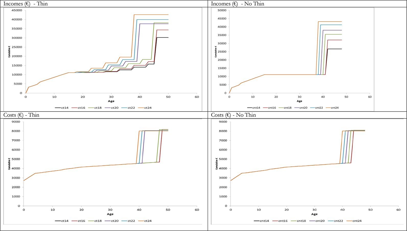
ForBES provides cost and income curves for thin and no-thin scenarios and generate annual equivalent NPVs for a range of discount rate, subsidy, thinning, rotation and indexation options. The life-cycle pattern of costs and incomes are presented graphically in Figure 2 Figure 2for establishing a Sitka spruce (SS) forest (which accounts for almost two thirds of non-industrial private forestry in Ireland) in 2015, across a range of productivity (yield) classes (yc).

Life-Cycle Pattern of Incomes and Costs by yield class over 1 rotation (2015) for conifer thin (ct) and conifer no thin (cnt) options
There is a considerable difference between the curves for the conifer thin (ct) and no-thin (cnt) scenarios. The distribution of income and cost in the early years of the rotation is the same for both thinned and unthinned crops, regardless of yield class, as early income is derived from grant and premium subsidies which are categorised only by species and not by site productivity. Across the yield classes, there is an almost incremental increase in income.
In this analysis, the reforestation cost of the next rotation is included as a cost in the first rotation and is evident in the substantial increase in costs after clearfell. While it can be argued that theoretically, the cost of reforestation should not be apportioned to the first rotation, from a pragmatic and transparency perspective, forest owners cannot achieve clearfell revenues without incurring the cost of reforestation. In reality, because the cost arises at the end of the rotation and is dwarfed by the clearfell revenue, it is unlikely to have much impact on the magnitude of the NPV.
4.1. Panel data models: on farm hours and land value per hectare
In understanding the impact of forestry planting on hours worked and land values, we estimate two panel data models using the Teagasc NFS which collects annual data on the number of hours worked (on and off-farm) and on farmer’s self-assessed land value. The model coefficients for the random effects panel data models necessary to impute counterfactuals for hours worked and land value reported (taking logs to remove the scale effects) are reported in Appendix 1—Table 2. The model outputs are consistent with a priori expectations in relation to how hours worked and land value change for different farm and farmer characteristics and have good explanatory power (Hours worked 33%, Land value 31%).
As expected, the coefficient on new forest planting is negative and significant, indicating a reduction in hours worked as a result of planting. In addition, the level of hours worked increases with farm size and is higher for farms with a greater share of livestock but lower for farms with a greater share of tillage (due to increased use of contractors).8 Hours worked is also positive for higher stocked farms on good to medium soils. As would also be expected, it is however lower for older farmers and those with off-farm employment.
Participation in the REPS agri-environment scheme results in increased work hours, a factor which was also noted by Murphy et al. (2014). The coefficients on farm size (positive) and farm size squared (negative) show that hours worked increases with increasing farm size but at a reducing rate. The age and age squared coefficients (both negative) show that the reduction in hours worked accelerates as farmers get older.
In the land value model, only those factors that affect land value are included. The most important information is that (conditional on the lagged value of land), the coefficient on new forest planting is significant and negative, indicating that afforestation reduces farmers’ (self-reported) perceptions of the value of planted land, while land value increases on farms with good to medium soils and on intensive farms with high livestock densities per hectare.
This is also consistent with a priori expectations based on the loss of flexibility of land use imposed by the legal requirement to replant forests once the timber is harvested. Although the land value is self-assessed, it provides a reliable indication of value. In a comparison of the annual NFS land values with annual agricultural land sales official statistics, a recent Irish study found that while the NFS values are below the official sales figures, the trend over time is almost exactly the same. This result is consistent with the authors experience in the forestry sector and is consistent with published Irish forest land sale prices9.
5. Results II: distributional analysis
The purpose of this analysis is to try to understand the impact of planting on the relativity of agriculture and forestry incomes and the impact on land values and hours worked. In our data, we observe the farms that have planted (has forest) and those that have not (no forest). In order to understand the drivers of forest planting behaviour, we first simulate the impacts of a marginal change in land use. We utilise the Teagasc ForBES and the ForSubs models to simulate forest market and subsidy income respectively and utilise the two reduced form econometric models described above to simulate counter factual land and labour impacts. However these averages mask significant heterogeneity across farms so we also disaggregate farms on the basis of whether the agricultural or forest income life cycle streams are greater over time for each farm in the population. Variables are generated whereby life cycle forest income streams are defined as annual equivalised (AE) NPV of market plus subsidy income and compared directly with agricultural incomes (on a per hectare basis). Agricultural life cycle income streams are defined as AE (NPV) of market income, farm gross margin and farm net margin (on a per hectare basis). These impacts are examined for both ‘has forest’ and ‘no forest’ farms. This categorisation is at the heart of this analysis as it is expected that the relativity of these life cycle incomes is a major driver in the afforestation decision.
Table 1 describes the average changes in income, land and labour which would result from the decision to plant a proportion of the farmland, simulating in turn, a straight land use change of five percent of the land, the change in value and the change in hours worked.
Impact of planting on income, land and labour
| Proportional change in | |||||
|---|---|---|---|---|---|
| Market income | Gross margin | Net margin | Land value | Hours worked | |
| No Forest | −0.1953 | −0.1397 | −0.25 | −0.051 | −0.034 |
| Has Forest | −0.1948 | −0.11396 | −0.246 | −0.034 | −0.033 |
We see that for each of the income types (market, gross margin and net margin), planting five percent of the farmland results in a slight reduction in income, (as expressed in terms of AE of NPV), as the income from forestry is lower on average than agricultural income. Hours worked reduces due to the lower time input required for forestry than for livestock farming, thus increasing leisure. Although the reduction in hours is small, this is consistent with the underemployment in Irish agriculture noted by Loughrey and Hennessy (2016). Land values show a small decrease on average due to preferences for farming and lower land flexibility, however given the contribution of land to the overall asset base, a 3%–5% fall in value is quite important.
To test the sensitivity of the results, we utilise data from 2012 to 2015 to compare the ratios for farms with forests against those without forests. The results are presented in Table 2 where farms with higher incomes from forestry than from agriculture (For> Ag) are also examined on the basis of the three agricultural income definitions. Finally, future planting intentions are examined, comparing farms that indicated they would ‘never plant’ (1) with those who might plant (never plant 0).
Proportion of Farms where the Forestry AE is greater than Agriculture AE
| Classification | Market income | Gross margin | Net margin |
|---|---|---|---|
| Has Forestry | |||
| 0 | 0.527 | 0.298 | 0.596 |
| 1 | 0.629 | 0.454 | 0.703 |
| Never Plant | |||
| 0 | 0.633 | 0.387 | 0.658 |
| 1 | 0.538 | 0.303 | 0.616 |
-
Source: Teagasc National Farm Survey 2012–2015 and Teagasc ForBES/ForSubs Models.
The proportion of farms that have a higher AE for forestry than agriculture is greater amongst those who have planted forests. This is true for each measure of income considered. Considering market income, 63% of farmers who planted had a higher AE for forestry than for agriculture. However the rate for those who have not planted forestry is 53%. Comparing forestry returns with the agricultural gross margin, where agricultural subsidies are included, the proportion falls to below 50%, with rates of 30% and 45% respectively for farms with and without forestry. When subtracting overhead costs (net margin), the share peaks at 70% and 60% respectively.
Turning to future intentions, we find similar conclusions. Of those who ‘might plant (corollary of never plant) , there are more farmers who have a higher AE from forestry than from agriculture. However as is the case for those farms that have already planted, the gap is relatively low, again indicating the heterogeneity of the underlying behavior.
Overall, there are substantial numbers of farmers who would be financially better off by planting, but who have not done so, while similarly there are substantial numbers of farmers who have planted, even when they would have been better off to retain all their land in agriculture. The former may be explained as a result of cultural factors underlying a reluctance to plant (Ní Dhubháin and Gardiner, 1994; Frawley and Leavy, 2001; Malone, 2008; O’Leary et al., 2000; McDonagh et al., 2010; Duesberg et al., 2013), while the latter cohort may be influenced by non-pecuniary factors.
In Table 3, we decompose the annual equivalised NPV into income components (average) for farms that have planted and those that have not. Where agriculture has a higher AE than forestry (Group A), the biggest difference is evident in farm income (output - direct costs), which is substantially different to those farms with a lower agricultural AE (Group B). This is partly due to the substantially higher incomes on dairy versus other systems and the fact that dairy farms are proportionally located on productive soils. Farm subsidies are higher for Group A but the gap is quite small. Overhead costs, consistent with productivity, have a similar pattern to farm incomes. The gap for forest income is relatively small, with potential forest income being slightly higher when the agricultural income is higher, as both agricultural and forest incomes are greater on more productive soils.
Components of Income 2012–2015 by relative AE
| Forest mkt income per Ha | Forest subs income per Ha | Farm income per Ha | Farm subsidy per Ha | Overhead cost per Ha | Difference MI | Difference GM | Difference NM | |||
|---|---|---|---|---|---|---|---|---|---|---|
| For > Ag* | Has forest | |||||||||
| A | 0 | 0 | 490 | 329 | 1,827 | 415 | 876 | −1008 | −1423 | −547 |
| 0 | 1 | 494 | 329 | 1,651 | 400 | 803 | −828 | −1228 | −426 | |
| B | 1 | 0 | 475 | 329 | 369 | 390 | 419 | 435 | 44 | 463 |
| 1 | 1 | 470 | 328 | 270 | 389 | 386 | 528 | 139 | 525 |
-
*
Farms where potential forestry income is greater than or equal to potential agricultural income
When we compare ‘has forest’ farms in Group A with ‘no forest’ farms, all income differences (forest – agriculture) are negative, but less negative for ‘has forest’ farms. The biggest driver of difference is lower agricultural incomes. For group B, the forest-agriculture income difference is higher for ‘has forest’ farms. Again the differential is primarily driven by farm income. In fact potential forest market income and subsidies are higher for ‘no forest’ farms, suggesting that forest policy is relatively untargeted from an incentive perspective.
In Table 4 we take the difference between forest and agricultural market incomes and group this difference into deciles, where higher deciles have a higher difference between forest and agricultural income. Plotting the probability of having a forest, we find that for ‘has forest’ farms, there is a substantial difference between the biggest gap (32%) and the lowest decile with only 7% difference. In general however, we see a relatively small difference in the planting rate between the 2nd and the 8th decile, indicating that financial incentives seem to only have an impact at the extremes of the distribution.
Deciles of gap between forest and agriculture (Market Income)
| Has forest | Never plant | |
|---|---|---|
| 1 | 0.073 | 0.924 |
| 2 | 0.153 | 0.854 |
| 3 | 0.168 | 0.877 |
| 4 | 0.163 | 0.883 |
| 5 | 0.136 | 0.820 |
| 6 | 0.118 | 0.824 |
| 7 | 0.189 | 0.853 |
| 8 | 0.172 | 0.849 |
| 9 | 0.238 | 0.799 |
| 10 | 0.319 | 0.798 |
The probability of never planting takes as expected, the opposite trend, being greater for the lowest gap and least for the highest gap. However the range between the top and the bottom is not as great proportionally as for ‘has forest’ farms.
While Table 4 considered probabilities for market incomes only, we next expand the analysis to examine the deciles across all three agricultural income measures for ‘has forest’ farms. The results presented in Table 5 indicate that while the trend is similar, the proportional range between decile 1 and 10 is smaller for the gross margin and net margin income measures. Thus, it would appear that the planting is more strongly influenced by the financial gain associated with the market income measure.
Deciles of forest–agriculture gap (Has Forest) by income definition
| Decile | Market income | Gross margin | Net margin |
|---|---|---|---|
| 1 | 0.073 | 0.065 | 0.091 |
| 2 | 0.153 | 0.180 | 0.135 |
| 3 | 0.168 | 0.157 | 0.161 |
| 4 | 0.163 | 0.138 | 0.154 |
| 5 | 0.136 | 0.132 | 0.117 |
| 6 | 0.118 | 0.176 | 0.179 |
| 7 | 0.189 | 0.150 | 0.206 |
| 8 | 0.172 | 0.247 | 0.227 |
| 9 | 0.238 | 0.208 | 0.242 |
| 10 | 0.319 | 0.276 | 0.211 |
| Total | 0.172 | 0.172 | 0.172 |
In Table 6, we examine the deciles of the difference between forest and agricultural incomes (forest minus agriculture) in relation to the individual components of income. The difference in forest income between decile 1 and 10 is relatively small for farm subsidies, with the biggest difference being due primarily to agricultural market incomes and to a lesser extent, to overhead costs. Thus it appears that farm income variability has a greater impact on financial drivers than forestry incomes. This raises an important policy question as to whether forest subsidies should be paid on a straight per hectare basis, or on the basis of the opportunity cost foregone from the superseded land use.
Income characteristics by decile of forest-agriculture gap (Market Income)
| No forestry | Forestry income per Ha | Farm income per Ha | Farm subsidy per Ha | Overhead cost per Ha | Difference MI | Difference GM | Difference NM |
|---|---|---|---|---|---|---|---|
| 1 | 825 | 2,974 | 407 | 1,176 | −2149 | −2555 | −1379 |
| 2 | 820 | 2030 | 386 | 970 | −1210 | −1595 | −625 |
| 3 | 819 | 1,550 | 409 | 808 | −731 | −1140 | −332 |
| 4 | 816 | 1,142 | 439 | 662 | −326 | −765 | −103 |
| 5 | 813 | 820 | 451 | 582 | −7 | −459 | 124 |
| 6 | 816 | 604 | 419 | 505 | 212 | −207 | 298 |
| 7 | 806 | 457 | 408 | 438 | 349 | −59 | 379 |
| 8 | 803 | 321 | 371 | 403 | 483 | 112 | 515 |
| 9 | 792 | 186 | 349 | 334 | 605 | 256 | 590 |
| 10 | 794 | −13 | 362 | 314 | 807 | 446 | 759 |
| 810.39 | 1007.02 | 400.04 | 619.04 | −197 | −597 | 22 | |
| Has Forestry | |||||||
| 1 | 821 | 2,876 | 403 | 1,120 | −2055 | −2458 | −1339 |
| 2 | 823 | 2083 | 389 | 942 | −1260 | −1648 | −707 |
| 3 | 825 | 1,574 | 371 | 777 | −749 | −1121 | −344 |
| 4 | 820 | 1,163 | 434 | 689 | −342 | −777 | −88 |
| 5 | 822 | 823 | 420 | 574 | −1 | −420 | 154 |
| 6 | 802 | 577 | 435 | 487 | 225 | −210 | 277 |
| 7 | 808 | 468 | 378 | 400 | 340 | −39 | 362 |
| 8 | 805 | 333 | 389 | 448 | 473 | 84 | 532 |
| 9 | 799 | 190 | 382 | 345 | 609 | 228 | 573 |
| 10 | 781 | −19 | 374 | 292 | 800 | 425 | 717 |
| 810.67 | 1006.78 | 397.50 | 607.30 | −196.10 | −593.61 | 13.69 | |
Finally, Table 7 describes the characteristics of farms by decile. The lowest deciles with the largest agriculture-forestry gap are more likely, unsurprisingly to have a greater share of higher income. These farmers are likely to be younger dairy farmers with more intensive systems and higher stocking rates, are more likely to pay for extension services, to be full time farmers and farming on better soils. The corollary also holds that those with a greater financial incentive to plant forests are more likely to be older, farming on marginal land in drystock systems and are more likely to work off-farm.
Farm/farmer characteristics by decile of forest-agriculture gap (Market Income)
| Decile | Family farm income per Ha | Dairy cows per Ha | Labour units | Age | Farm size | Teagasc | Has reps | Has off farm income | Best soil type |
|---|---|---|---|---|---|---|---|---|---|
| No Forestry | |||||||||
| 1 | 1,652 | 2.36 | 1.39 | 50 | 57 | 0.75 | 0.25 | 0.51 | 0.72 |
| 2 | 1,085 | 1.88 | 1.42 | 53 | 71 | 0.72 | 0.15 | 0.45 | 0.65 |
| 3 | 880 | 1.48 | 1.36 | 54 | 67 | 0.68 | 0.27 | 0.52 | 0.65 |
| 4 | 717 | 0.73 | 1.28 | 57 | 66 | 0.63 | 0.22 | 0.57 | 0.61 |
| 5 | 548 | 0.24 | 1.18 | 56 | 56 | 0.57 | 0.24 | 0.68 | 0.57 |
| 6 | 419 | 0.15 | 1.14 | 58 | 54 | 0.56 | 0.15 | 0.64 | 0.62 |
| 7 | 357 | 0.05 | 1.08 | 58 | 53 | 0.54 | 0.14 | 0.65 | 0.52 |
| 8 | 239 | 0.04 | 1.06 | 58 | 46 | 0.45 | 0.18 | 0.62 | 0.48 |
| 9 | 174 | 0.01 | 1.01 | 58 | 48 | 0.45 | 0.20 | 0.67 | 0.38 |
| 10 | 51 | 0.03 | 1.11 | 60 | 87 | 0.36 | 0.09 | 0.67 | 0.41 |
| 612.13 | 0.70 | 1.20 | 56.22 | 60.49 | 0.57 | 0.19 | 0.60 | 0.56 | |
| Has Forestry | |||||||||
| 1 | 51 | 0.03 | 1.11 | 60 | 87 | 0.36 | 0.09 | 0.67 | 0.41 |
| 2 | 1,629 | 2.39 | 1.37 | 51 | 61 | 0.82 | 0.11 | 0.66 | 0.64 |
| 3 | 1,157 | 1.98 | 1.49 | 53 | 78 | 0.70 | 0.14 | 0.52 | 0.67 |
| 4 | 929 | 1.48 | 1.41 | 53 | 84 | 0.72 | 0.18 | 0.56 | 0.71 |
| 5 | 724 | 1.01 | 1.50 | 55 | 89 | 0.57 | 0.40 | 0.55 | 0.65 |
| 6 | 546 | 0.53 | 1.52 | 55 | 74 | 0.78 | 0.30 | 0.45 | 0.68 |
| 7 | 462 | 0.14 | 1.23 | 55 | 70 | 0.62 | 0.28 | 0.56 | 0.44 |
| 8 | 403 | 0.04 | 1.02 | 56 | 52 | 0.69 | 0.16 | 0.77 | 0.49 |
| 9 | 255 | 0.09 | 1.02 | 54 | 68 | 0.71 | 0.15 | 0.67 | 0.49 |
| 10 | 270 | 0.01 | 1.15 | 56 | 67 | 0.69 | 0.24 | 0.75 | 0.44 |
| 642.51 | 0.77 | 1.28 | 54.84 | 72.85 | 0.67 | 0.21 | 0.61 | 0.56 | |
6. Conclusions
This paper describes a static microsimulation approach which provides a better understanding of the life-cycle relativity of forestry and agricultural incomes, using Ireland as a case-study. Due to the complexity and micro data requirements, there is a general gap in the land use change literature in relation to modelling at the individual farm level. The unique contribution of the microsimulation approach taken in this paper is that it combines two units of micro analysis, namely the farm and the forest. While there are existing studies in the literature that individually model farm and forest level incomes, studies that examine the incomes from both land-uses are limited. However, information on both land uses is necessary to understand such a major and permanent land use change. This analysis examines both private (market) and public (subsidy) income sources arising from farming and forestry activities. In combination, these different income sources produce a high degree of heterogeneity, leading to very detailed farm level results.
The static microsimulation methodology allows for the generation of actual and counterfactual forest and agricultural income streams and for other attributes of utility such as long-term wealth and leisure, for the first time. Income variables are generated to directly compare the life-cycle income streams from agriculture and forestry (on a per hectare basis) given the agronomic and environmental conditions of individual farms.
The results show that financial drivers are significant and important drivers of farm afforestation as the proportion of farms with greater life-cycle income streams from forestry is higher amongst farmers who have already planted. The results also show that substantial numbers of farmers would be financially better off to plant forests, however many of these farmers have not planted. Malone (2008) recognizes that the decision to change from agriculture to forestry on a parcel of land is not taken in isolation and lists multiple factors including personal circumstances, the relative attraction of available subsidies and the permanent nature of the decision, which removes other options for land use and has implications for current and future generations. The static microsimulation methodology utilised in this study to quantitatively determine the economic implications of planting referred to by Malone (ibid.), has not previously been used in the agriculture to forestry land use change context.
While previous afforestation incentives focused only on horizontal policies, this analysis suggests that policies that are targeted to take account of direct (financial) and non-direct (lifestyle and land use flexibility) drivers of afforestation, may be more effective in increasing the uptake of farm afforestation. It is evident that the differential between potential forest and agricultural income is driven primarily by farm income, while planting behaviour is more strongly influenced by the financial gain associated with the market income measure. This raises an important policy question as to whether forest subsidies should be paid on a straight per hectare basis, or on the basis of the opportunity cost of the alternative land use. It would further appear that forest policy is relatively untargeted from an incentive perspective and that the financial incentives seem to only have a strong impact at the extremes of the distribution of farms in relation to income potential. This suggests that targeted incentives might be more effective than the horizontal incentives that have previously applied across all farms irrespective of system and income levels.
The average decrease in land value reported by farmers after planting reflects the inter-temporal commitment and loss of flexibility of land use associated with afforestation. While the permanent nature of forestry as a land use has been cited as a barrier to planting (McDonagh et al., 2010) the decrease in self-assessed land value has not previously been quantified.
As the afforestation of agricultural land is now a primary component of the climate change mitigation tool kit, methodologies that provide greater understanding of individual farm level economic drivers that could be manipulated to incentive the necessary land use change are increasingly important. The methodology presented here is relevant for Ireland, but the framework employed uses Irish FADN data collected by the Teagasc National Farm Survey and thus has potential for cross country comparative analysis using FADN data. Thus the methodology is readily scaleable to the EU level and potentially globally. In the broader context of Climate Smart Agriculture and the Grand Challenges facing the intensification of agricultural production, these findings have implications for policies that seek to optimise natural resource use.
Footnotes
1.
In the EU 28, forests cover a slightly higher proportion of land area (42.4%) than that which is used for agriculture.
2.
For example, UK forest expansion has dropped back from a high of 40,000 hectares (ha) per year in the early 1970s to an average of about 10,000 ha per year (Forestry Commission, 2013) and Dutch expansion targets will not be realized (Van Gossum et al., 2010) and afforestation in Flanders is falling (Van Gossum et al., 2012).
3.
We ignore here the case of complex transition arrangements where in some periods subsidies from agriculture and forestry can be stacked together.
4.
NPV (Net Present Value) is the sum of the present values of incoming and outgoing cash flows over a period of time. Incoming and outgoing cash flows can also be described as income and cost cash flows.
5.
LFA (Less Favoured Areas) payment: higher subsidies were paid on farms designated as ‘more severely handicapped’ for some of the period.
6.
Cost and revenue assumptions employed in the analysis are detailed in Appendix 1—Table 1.
7.
Trees may be removed or ‘thinned’ at 5 year intervals providing an interim income, or may remain ‘unthinned’, with revenue arising only at final clearfell.
8.
In order to address commonly occurring multicollinearity between predictor values such as farm size and number of livestock units, the model estimation includes a variable to examine livestock units per hectare, thus capturing additional information over and above the farm scale effects.
9.
10.
The land value per hectare explanatory variable is logged and lagged, reflecting the logged dependent variable.
Appendix 1
Teagasc ForBES Model : Detailed Cost assumptions
| SS (€/ha) | Ash (€/ha) | |||
|---|---|---|---|---|
| Forest establishment | % of costs covered by Afforestation Grant dependent on year of planting | Allocated to Year 0 | 2,860 | 4,280 |
| Forest maintenance up to end year 4 | Costs covered by Maintenance Grant | Payment allocated equally over years 1,2,3 & 4 | 790 | 1,155 |
| Annual management cost | Incurred annually | 20 | 20 | |
| Insurance | Initial payment in year 5 – runs to year 20 | Recurring annually | 20 | 20 |
| Brash/inspection paths | One-off cost of cutting inspection paths through conifers Not relevant for ash | Incurred in year 14 | 35 | 0 |
| Second fertiliser | Relevant only for unenclosed sites with additional nutrient requirements | Not relevant for SS-GPC3 or for ash | ||
| Cost of Sales | % reduction in revenue | Lower in high value sites | Clearfell –12% | Clearfell – 12% |
| Road costs | Only applicable if thinning | Not necessary in many small farm forests | Assume that road grant covers cost | 0 |
| Harvest losses | Timber losses due to difficult site conditions | Binary – Yes/No | 1st Th: 14%
2nd TH: 12% 3rd /sub TH: 8% C/fell: 5% |
|
| Reforestation | Cost of replanting with same species post clearfell | May be allocated to first or second rotation | 3,500 | 0 |
Model Estimates, On-Farm Hours and Land Value per hectare10
| Logged (On-Farm Hours Worked) | Logged (Land Value per ha) | |||
|---|---|---|---|---|
| Variables | Coefficient | SE | Coefficient | SE |
| New forest planting | −0.0351*** | −1.72 | −0.0529* | 0.0293 |
| Land Value (lagged : t-1)/ha | −0.0299*** | −6.35 | 0.0075*** | 0.0008 |
| Farm Size | 0.0009*** | 6.21 | −0.0071*** | 0.0002 |
| Farm Size Squared | −0.000001*** | −4.24 | *** | 0 |
| Age | −0.0053*** | −24.76 | ||
| Age Squared | −0.000003*** | −19.03 | ||
| Has Off Farm Employment | −0.1731a | −32.25 | ||
| Spouse Has Off Farm Employment | 0.019** | 3.35 | ||
| Share of Tillage Area | −0.0966*** | −4.08 | 0.1257*** | 0.0331 |
| Share of Dairy Forage | 0.2241 | 11.12 | −0.0658** | 0.0286 |
| Share of Sheep Forage | 0.049* | 2.91 | −0.0782a | 0.0242 |
| Sheep Number of Livestock Units per ha | 0.0049** | 1.82 | 0.001 | 0.0041 |
| Cattle Number of Livestock Units per ha | 0.0294** | 6.89 | 0.0313*** | 0.0066 |
| Dairy Number of Livestock Units per ha | 0.001** | 0.16 | 0.0435*** | 0.0089 |
| Teagasc Client | −0.01*** | −2.22 | ||
| Has REPS payment | 0.0133** | 2.46 | ||
| Unpaid labour | 0.4188 | 66.04 | ||
| Good soil | 0.463*** | 0.0246 | 0.0455* | 2.66 |
| Medium soil | 0.2435*** | 0.0243 | 0.0352* | 2.11 |
| Constant | −0.4719*** | 0.0197 | 7.1293 | 3.65 |
| Share of Variance due to Fixed Effect | 0.58 | 0.69 | ||
| R2 | 0.3309 | 0.3021 | ||
| N | 29,567 | 27,219 | ||
-
Note: Regional, Soil and Year dummies ignored.
-
***significant at 1% level;* significant at 10% level
References
-
1
Econometric studies of non-industrial private forest management: a review and synthesisForest Policy and Economics 7:261–281.https://doi.org/10.1016/S1389-9341(03)00065-0
-
2
Discrete Choice Analysis: Theory and Application to Travel DemandCambridge, Ma: MIT Press.
-
3
Irish land use change and the decision to afforest: an economic analysisIrish Forest 67:6–20.
-
4
Economics of Irish Forestry: Evaluating the Returns to Economy and SocietyDublin: COFORD.
-
5
Offsetting New CO2 Emissions: A Rational First Greenhouse Policy StepContemporary Policy Issues 8:29–41.
-
6
Assessing policy tools for encouraging farm afforestation in IrelandLand Use Policy 38:194–203.https://doi.org/10.1016/j.landusepol.2013.11.001
-
7
To plant or not to plant—Irish farmers’ goals and values with regard to afforestationLand Use Policy 32:155–164.https://doi.org/10.1016/j.landusepol.2012.10.021
- 8
-
9
Modelling farmer decision-making: concepts, progress and challengesAnimal Science 82:783–790.https://doi.org/10.1017/ASC2006112
-
10
Yield Models for Forest ManagementYield Models for Forest Management, Forest Commission Booklet 48, HMSO, London.
-
11
Farm woodland policy: an assessment of the response to the farm woodland scheme in Northern IrelandJournal of Environmental Management 34:197–209.https://doi.org/10.1016/S0301-4797(05)80151-3
- 12
-
13
Berechnung des Werthes, welchen Waldboden, sowie noch nicht haubare Holzbestände für die Waldwirthschaft besitzenAllgemeine Forst- und Jagd-Zeitung 25:441–455.
- 14
-
15
Forest statisticshttp://www.forest.gov.uk/website/forstats2013, [Accessed Jan 2014].
- 16
-
17
Social security money’s worthSocial security money’s worth, NBER Working Paper Series 6722.
-
18
The Australian farm forestry financial modelAustralian Forestry 72:184–194.https://doi.org/10.1080/00049158.2009.10676300
- 19
-
20
Handbook of Microsimulation Modelling449–477, Environmental Models, Handbook of Microsimulation Modelling, Emerald Group Publishing Limited.
-
21
Average and marginal effective tax rates facing workers in the EU: A micro-level analysis of levels, distributions and driving factorsAverage and marginal effective tax rates facing workers in the EU: A micro-level analysis of levels, distributions and driving factors, OECD Social, Employment and Migration Working Papers, No. 19.
-
22
FALLING up the stairs: the effects of "bracket creep" on household incomesReview of Income and Wealth 51:37–62.https://doi.org/10.1111/j.1475-4991.2005.00144.x
-
23
Annuity markets in comparative perspective: do consumers get their money’s worth?Annuity markets in comparative perspective: do consumers get their money’s worth?, Policy Research Working Paper 2493.
- 24
-
25
Handbook of Microsimulation Modelling47–75, Static Models, Handbook of Microsimulation Modelling, Contributions to Economic Analysis, Volume 293, Emerald Group Publishing Limited.
-
26
Farm income variability and off-farm employment in IrelandAgricultural Finance Review 76:378–401.https://doi.org/10.1108/AFR-10-2015-0043
- 27
-
28
Economic determinants of private afforestation in the Republic of IrelandLand Use Policy 20:51–59.https://doi.org/10.1016/S0264-8377(02)00052-2
-
29
Missed opportunity or cautionary steps? farmers, forestry and rural development in IrelandEuropean Countryside 4:236–251.
-
30
Conditional Logit analysis of qualitative choice behaviourFrontiers of Econometrics.
-
31
Policy options for afforestation in FlandersEcological Economics 64:194–203.https://doi.org/10.1016/j.ecolecon.2007.02.021
-
32
Costs of sequestering carbon through tree planting and forest management in the U.SWashington DC: U.S. Department of Agriculture, ForestService, Gen. Tech. Rep. WO-58, December 1990.
-
33
The participation decision in the rural environment protection scheme (REPS): a conditional logit approach using simulated counterfactual data for farmersPaper presented to European Association of Agricultural Economists Congress.
- 34
-
35
Do tax-benefit systems cause high replacement rates? a decompositional analysis using EUROMODLabour 25:126–151.https://doi.org/10.1111/j.1467-9914.2010.00501.x
-
36
Farm-Level Microsimulation ModellingFarm-Level Microsimulation Modelling, Palgrave Macmillan, ISBN:, 978-3-319-63978-9.
-
37
Afforestation in Ireland — regional differences in attitudeLand Use Policy 17:39–48.https://doi.org/10.1016/S0264-8377(99)00036-8
-
38
Economic issues in Irish forestryJournal of the Statistical and Social Inquiry Society of Ireland XXVI:179–209.
-
39
The Handbook of Microsimulation Modelling. Contributions to Economic Analysis, Vol 293(Ed), The Handbook of Microsimulation Modelling. Contributions to Economic Analysis, Vol 293, ISBN:, 978-1-78350-589-2.
-
40
A guide to the valuation of commercial forest plantationsA guide to the valuation of commercial forest plantations, Dublin, COFORD, ISBN:, 978-1-902696-72-0.
-
41
Tightropes and tripwires: new labour’s proposals and means-testing in old ageCASE paper 23, Centre for Analysis of Social Exclusion, London School of Economics.
-
42
Handbook of microsimulation modelling505–534, Farm level models, Handbook of microsimulation modelling, Emerald Group Publishing Limited.
-
43
The role of subsidy payments in the uptake of forestry by the typical cattle farmer in Ireland from 1984 to 2012Irish Forestry 71:92–112.
-
44
Modelling financially optimal Afforestation and forest management scenarios using a Bio-Economic modelOpen Journal of Forestry 06:19–38.https://doi.org/10.4236/ojf.2016.61003
-
45
Land use change from agriculture to forestry: a structural model of the income and leisure choices of farmersInternational Association of Agricultural Economists. 2015 Conference.
-
46
Management Data for Farm Planning. Annual Editions. (1984 to 2012)Various years, Management Data for Farm Planning. Annual Editions. (1984 to 2012), Oak Park, Carlow, Teagasc.
-
47
An analysis of money’s worth ratios in ChileJournal of Pension Economics and Finance 6:287–312.https://doi.org/10.1017/S1474747207003150
-
48
Examining the relative competitiveness of milk production: an Irish case study (1996–2004)Journal of International Farm Management 3:49–61.
-
49
The potential economic returns of converting agricultural land to forestry: an analysis of system and soil effects from 1995 to 2009Irish Forestry 70:61–74.
-
50
Implementation of the forest expansion policy in the Netherlands in the period 1986–2007: decline in success?Land Use Policy 27:1171.https://doi.org/10.1016/j.landusepol.2010.03.007
-
51
“Smart regulation”: Can policy instrument design solve forest policy aims of expansion and sustainability in Flanders and the Netherlands?Forest Policy and Economics 16:23–34.https://doi.org/10.1016/j.forpol.2009.08.010
Article and author information
Author details
Funding
No specific funding for this article is reported.
Acknowledgements
Not applicable.
Publication history
- Version of Record published: August 31, 2019 (version 1)
Copyright
© 2019, Ryan and O’Donoghue
This article is distributed under the terms of the Creative Commons Attribution License, which permits unrestricted use and redistribution provided that the original author and source are credited.