Spatial microsimulation of osteoarthritis prevalence at the small area level in England – Constraint selection for a 2-stage microsimulation process

Spatial microsimulation methodologies represent a powerful tool used to create and analyse spatially disaggregated data without expending the vast resources required to obtain these data through primary data collection. Spatial microsimulation models could be static (looking at just one point in time), or dynamic (including projections overtime), and could be deterministic (does not incorporate random variability) or stochastic (incorporating random variability). There are several published reviews on the description, strengths and weakness of various spatial microsimulation methodologies (O’donoghue et al., 2014; Tanton, 2014; Birkin and Clarke, 2011; Rahman et al., 2010; Harland et al., 2012). This paper focuses on static deterministic spatial microsimulation models.

Static deterministic spatial models have the added advantage of the ability to conduct powerful counterfactual scenario modelling (Tanton, 2014). This is a modelling technique where the effect of input parameter manipulation can be assessed in the derived synthetic dataset. For example how would a 20% increase in the population of people in the lowest deprivation quintile affect the prevalence of obesity in a given geographical area? This can provide policy makers and researchers an insight into the potential effect of an intervention or policy across various geographical areas before the intervention/policy is implemented. This process could be described as mimicking the effect of a randomised control trial, without the attendant time and resources required to conduct one in real-time (Prakash et al., 2017). With such a powerful tool at our disposal and with the improvement in computational power making it easier to carry out complex calculations quickly and more effectively, it is no surprise that the number of published literature on applications of spatial microsimulation/microsimulation have increased exponentially in the past few years. These models have found use in various disciplines ranging from transport, economics, fiscal policy and even healthcare and demography (Smith et al., 2011; Ballas et al., 2006; van Leeuwen and Dekkers, 2013; Lovelace et al., 2014; Lymer et al., 2008; Rephann and Holm, 2004).

That being said, penetration of spatial microsimulation modelling into core medical and epidemiological research has been rather slow. We recognise that microsimulation methodologies have been used extensively in infectious disease epidemiology however these models typically dynamic and conducted at much coarser geographical levels and therefore lacking the small areal level spatial component (Habbema et al., 1996; Morris and Kretzschmar, 2000). Also, available published literature on spatial models used to simulate health conditions like smoking, obesity and osteoarthritis, these studies have found little use outside the microsimulation community (Edwards and Clarke, 2009; Smith et al., 2011; Cataife, 2014). We believe that this may be due to an inherent weakness in static, deterministic spatial microsimulation methodologies – Data limitations (Tanton and Edwards, 2012). This could either be differences in variable definitions in the geographical and population dataset or complete absence of certain predictor variables in the geographic and/or population dataset. The latter is of particular importance as it may affect the accuracy of the simulated dataset and constrain further analysis of the derived microdata (Cassells et al., 2013). This is explained as follows – in order to generate microdata at the required geographical scale typically two datasets are required, the population dataset (which contains the outcome of interest) and the geographical dataset (which contains the geographical identifier). Here, observations (in this case people) are assigned to geographical areas based on matched attributes shared between the two datasets for example the geographical dataset (usually the census) and the population dataset can be matched based on sex, age and ethnicity (Ballas et al., 2005). This means that these attributes selected should be associated with the outcome of interest and must be present in both datasets (Edwards and Clarke, 2009).

Demographic variables such as age, sex, ethnicity and social class may be sufficient to simulate certain outcomes however simulation of medical conditions generally require more information and this information that may not be collected in one single survey. For example, it may not be accurate to simulate the spatial prevalence of lung cancer based on age and sex alone, without collecting smoking history because smoking is a well-documented risk factor for lung cancer (Doll and Hill, 1950; Doll and Hill, 1956; Lee et al., 2012). However, smoking data may not be available in the geographical dataset as only a few countries collect small area level smoking data. This means that it may not be possible to conduct an accurate spatial microsimulation model of lung cancer or convince policy makers about the validity of the resulting dataset.

Several methods have been employed to overcome this challenge ranging from imputation (Cassells et al., 2013) in the case of missing benchmark variables in the survey dataset, to merging geographically disaggregated data from another source with census data (where important predictor variables are missing from the census data) (Edwards and Clarke, 2009). Although these methods were appropriate in the situations in which they were used, and simulated outputs were found to be robust, these methods may not be applicable in all scenarios for example in the case of lung cancer mentioned above where smoking history data is unavailable in the census dataset and not accessible from other sources.

Univariate and Multivariate logistic regression were used to identify associations between knee osteoarthritis and other covariates. All significant predictors of knee OA identified during the univariate analysis (adjusted Wald’s test, p ≤0.05) were included in a multivariate backward elimination regression analysis. Only predictors (except age and sex, which were considered as priori predictors and retained in the model regardless of statistical significance) with a p value of ≤0.05 were left in the final model. We reinserted excluded predictors to the final model one at a time to further check whether they became statistically significant.

An optimal number of constraint variables is necessary to obtain accurate synthetic data however more constraint variables are not necessarily associated with accurate simulations (Tanton and Vidyattama, 2010). As an additional step, calibration was done by testing different combinations of variables in the final model using the Archer-Lemeshow goodness of fit test (Archer et al., 2007; Williams, 2015). Variables in the model with the highest p value were selected as constraint variables.

HSE 2012–2014 were combined to increase the size of the survey population, potentially increasing the pool of individuals to choose from during spatial microsimulation modelling. Multinomial logistic regression, with BMI as the outcome variable was used to identify covariates associated with BMI. Variables found to be significantly associated with BMI using multivariate multinomial regression were retained. We were unable to statistically compare nested models to obtain the most parsimonious model because maximum likelihood assumptions that underpin these tests are violated by complex sampling designs used in HSE (Hahs-Vaughn et al., 2011; Williams, 2015). Therefore, we employed the following approach to final constraint selection. All retained covariates were chosen as constraints and used to simulate BMI data in different combinations, dropping and adding each variables in turn except age and sex which were included in all simulations. The resultant synthetic datasets were internally validated against predetermined criteria (described below), discarding configurations that did not meet our criteria. Covariates in the dataset with the best validation scores was selected as final constraint variables (Smith et al., 2007).

A single stochastic imputation using a chained equation approach based on candidates with complete data (age and sex) was used to replace missing data (Cassells et al., 2013). Data was assumed to be missing at random (Sterne et al., 2009; Marston et al., 2010). Variance Inflation Factor (VIF) test was used to detect multiple collinearity among variables in the regression models. We did not find any value above 10.

5.1. Spatial microsimulation

Our project used SimObesity, a static spatial microsimulation model developed within the School of Geography, University of Leeds. It utilizes a deterministic combinatorial optimisation procedure. Models like SimObesity have been used extensively in healthcare modelling and have been shown to produce robust estimates (Burden and Steel, 2016; Kosar and Tomintz, 2014). In addition, these models are simple and relatively quick to execute. A detailed description of the exact algorithm and applications of SimObesity can be found elsewhere (Edwards and Clarke, 2009; Timmins and Edwards, 2016). Briefly, SimObesity works in two steps. The first step determines the combination of individuals in a geographical area using the reweighing algorithm. The second step involves intergerisation so only ‘whole’ individuals and not fractions of people are assigned to each geographical area (Ballas et al., 2005). SimObesity algorithm is displayed in the equation below.

For P_{i j}

(1) ${\displaystyle x_{ij}=w_{ij}\times c_{ij}/s_{ij}}$

(2) ${\displaystyle y_{ij}=x_{ij}\times \sum c_j/\sum x_j}$

Where, P_ij represents each person in the population dataset.

x_{i j} is the reweight value for person i in area j.

w_{i j} is the person’s original weight in the population table for the first constraint variable and is the resulting weight (y_{i j}) from the previous constraint for all subsequent constraint variables.

c_{i j} is element ij of the corresponding constraint table.

s_{I j} is element ij of the corresponding summary table.

∑c_j is the sum of the relevant area column for the constraint variable.

∑x_j is the sum of the relevant area column for the reweight value calculated in the previous step.

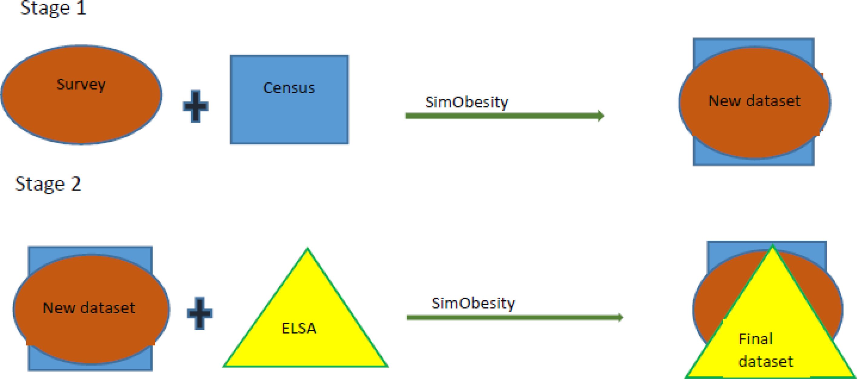
In our study, spatial microsimulation was conducted in a two-step sequence. First, constraints selected from the HSE analysis (described above) were combined with the 2011 Census (geographical dataset) using SimObesity to create a dataset that we called the hybrid dataset. This hybrid dataset contained information on both sociodemographic variables and BMI. Step 2 of the sequence involved combining the hybrid dataset with ELSA, also using SimObesity (based on constraint variables identified during the ELSA regression analysis) to obtain the final dataset. This dataset contained both knee OA data as well as BMI data. This processes illustrated in Figure 1 below. Initial (default) weights were set at ‘1’ for all simulations (Smith et al., 2009).

Figure 1

Download asset Open asset

This is an integral part of spatial microsimulation and there are broadly two approaches - internal and external. Internal validation examines how well the simulated data represents source data (constraint variables), while external validation tries to establish how closely the simulated estimates represent the actual spatial distribution of the outcome of interest. This is very challenging (hence the need for spatial microsimulation in the first place) (Edwards and Tanton, 2012).

Although several statistical techniques exist to internally validate spatial models, there is no consensus on which method is most appropriate. A review of the pros and cons of common internal validation techniques can be found in published literature (Timmins and Edwards, 2016; Rahman et al., 2013). In general, multiple techniques are used for internal validation. Our approach to validation was based on the simplicity of interpretation, preferring methods with an objective statistical measure over methods with a subjective interpretation.

Our simulated datasets were validated against the original census data ie, the hybrid and final dataset were each validated against the census data. This way we could access how close or removed our final dataset was from the census data. This was done with the following measures: R², Standard Absolute Error (SAE), and Standard Error about Identity (SEI) (Tanton and Vidyattama, 2010). Scatterplots were also used to visualize the relationship between simulated and census data. R² and SEI values ≥0.98, and SAE ≤0.05 were considered to be a good fit to generate the hybrid data, and R² and SEI values ≥0.94 and SAE values ≤0.10 to generate final knee OA dataset (Smith et al., 2009). R² and SEI cut off points were chosen pragmatically to account for a slight decay in the values at the second stage of simulation which may be caused by the intergerisation phase of SimObesity.

Prior to the validation methods mentioned above, we broadly compared constraint variables across all datasets i.e., we compared proportions of subgroups within all constraint variables in the hybrid dataset with those of the census and final datasets respectively. In addition, we aggregated the estimated data to a higher spatial scale, Government Office Region (GOR) and compared the proportion of people with knee osteoarthritis in ELSA (our final population dataset) with that of our synthetic dataset.

Data cleaning, constraint selection and model validation were conducted using STATA 14 SE (Statacorp, 2015) and Spatial microsimulation was done using SimObesity. Ethical approval was obtained from the University of Nottingham Ethics Committee SDA23062015.

There were a total of 9,169 core ELSA sample members, 12,521 observations from a combination of HSE 2012–2014, and about 18 million individuals in the 2011 census aged 50 years and above.

Table 2 below shows that the distribution of variables in all the 3 datasets is broadly similar with only slight differences in the frequency distribution of ‘separated’ individuals in ELSA compared with the Census and HSE. The frequency distribution of Education qualification also differs slightly between census, and HSE and ELSA datasets. However overall, HSE and ELSA are broadly representative of the census data making them ideal for spatial microsimulation.

Tables 3 and 4 below display the output of ELSA univariate and multivariate logistic regression analysis and GOF test respectively. Age, Sex, NSSEC, Health status and BMI were found to be significantly associated with Knee OA in the Univariate analysis.

Although Age was not significantly associated with Knee OA in multivariate analysis, it was considered to be an important predictor and thus included in the final model. Table 3 shows the results of the archer-Lemenshow Goodnesss of Fit (GOF) statistic. Comparing different combinations of variables in the final model – Age, Sex, NSSEC and BMI were shown to be the best predictors of knee OA, with the highest GOF p value of 0.9742. This is consistent with current available literature on the predictors of knee OA (Hart et al., 1999; Reyes et al., 2015; Blagojevic et al., 2010) therefore these variables were selected as constraint variables for knee OA spatial simulation modelling.

Table 5 above shows the results of multivariate multinomial regression analysis of HSE data. Age, Sex, NSSEC, Health, Marital status, Ethnicity, Highest Qualification, and Smoking status were identified as constraint variables. The census does not collect smoking status data, so smoking was not used as a constraint variable.

Age, Sex, NSSEC, Health, Marital Status, Ethnicity, and Education were used in different combinations as constraint variables to predict BMI. The Age, Sex and NSSEC simulation model provided the best fitted dataset based on our validation criteria and is the only result presented here. See following tables.

From Table 6 above, we can see that both the hybrid and final datasets have similar proportions of variables as the original census and HSE, and ELSA datasets (for BMI and Knee OA respectively)

Table 7 above displays internal validation measures at both simulation stages. It can be seen that in general, there was a slight reduction in SEI and R² values, and an increase in SAE values from the hybrid (BMI simulations) to the final dataset (OA simulations). All BMI simulations met our validation criteria of an SAE of ≤0.05 and R² value of ≥0.98, however age-group ≥90 years and males just failed to meet our set SEI criteria of ≥0.98. In the final simulations, age group ≥90 years also failed to meet our SAE and SEI criteria; and all sex sub-categories did not meet our set criteria as well. However, it can be observed that most sub categories of constraint variables met our validation criteria at both stages of the microsimulation sequence.

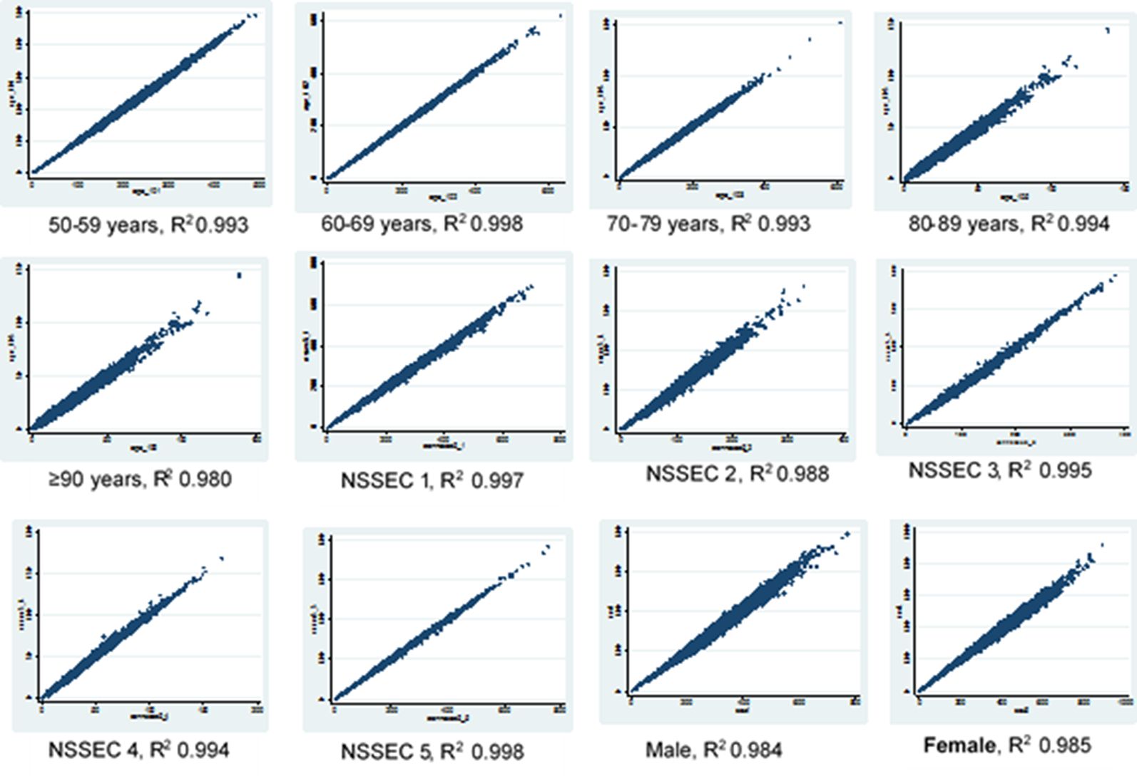
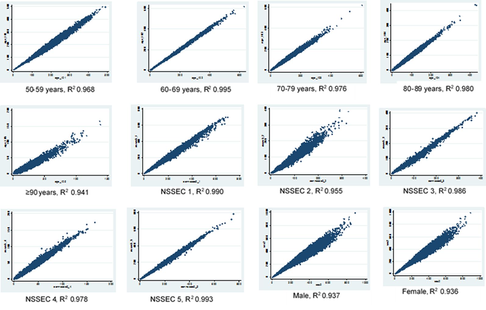
The results of the scatter plots above show a good correlation between the original census dataset and the final knee OA simulated dataset howbeit with a lower R² value for all constraint variable than obtained when the census was compared with the hybrid dataset (Figures 2 and 3). This effect is more pronounced in the sex category and in the age group 90 years and above. However the scatter plots show similar patterns across the different variables in both datasets which shows that the census data is correlated with the final OA simulation data.

Figure 2

Download asset Open asset

Figure 3

Download asset Open asset

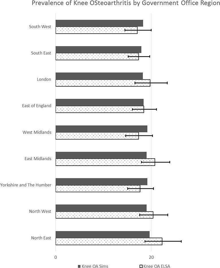
Figure 4 above compares the proportion of individuals with knee osteoarthritis from ELSA with that generated through spatial microsimulation. The error bars represent 95% confidence intervals. It can be seen here that synthetic data point estimates of the prevalence of knee osteoarthritis are within 95% confidence limits across all GORs. The highest difference of 2.7% points was seen in the North-East of England, with almost a perfect match in the East of England. ELSA proportions also appear to show more variability that the simulated data.

Figure 4

Download asset Open asset

The case study described above provided a detailed account of constraint selection and internal validation of a novel approach to spatial microsimulation. It demonstrated our approach to overcoming a key challenge encountered when generating small area level microdata. To this end, BMI, a variable found to be strongly associated with knee OA (from a literature search and our regression analyses) (Blagojevic et al., 2010) but not collected by our geographical dataset was successfully incorporated into the simulation by conducting simulations in 2 stages. This served a dual purpose because combining data from two survey datasets inadvertently increased the pool of individuals to choose from, as well as providing data on hitherto unavailable information. Although there seemed to be some ‘decay’ in validation scores in the final output, as shown by the slight increase in SAE and reduction in the R² values in the final dataset, the association between constraint variables in the census and final datasets is still very strong.

In addition, the proportions of individuals in various categories (of both constraint and outcome variables) were very similar across both survey datasets, hybrid and final datasets. It is also interesting to note that categories with only few observations (e.g. individuals aged 90 years and above) showed a poorer fit than categories with a large number of observations (50–59 years) in both the hybrid and final simulations. This also attests to the strong correlation between the original census and final datasets. Furthermore, the prevalence of our outcome of interest derived from our synthetic data approximated that derived from ELSA, with the largest point estimate difference of less than three percentage points. Another strength of this approach is that the similarity of source datasets such that individuals in the HSE and ELSA are alike in terms of variable categorization and sampling framework probably making it easier to clone individuals based on selected attributes however HSE contained slightly higher absolute numbers of participants in each category.

Bearing this in mind, it is also important to highlight some important considerations – first, the case study described above was conducted using a static deterministic reweighing and combinatorial spatial microsimulation method. It may not be applicable to other reweighing spatial simulation methods e.g. methods utilizing iterative proportional fitting, and other dynamic spatial models.

Secondly, choice of constraint is a very important determinant of the simulated output. Any other selection of constraints would produce a different output however our choice of constraint variables were based on correlates of the outcome of interest using robust calibration techniques. Our final choice of simulation output was based on predetermined internal validation criteria. In addition, some variables such as presence of long term illness and smoking history which were significantly associated with BMI in our regression analysis were not used as constraint variables to obtain the hybrid dataset. This is because the UK census does not collect data on smoking prevalence and also a systematic review of published literature has shown an inconclusive relationship between smoking and Osteoarthritis, our main outcome of interest (Hui et al., 2011; Hart et al., 1999). The presence of long term illness was not defined consistently across datasets and therefore could not be used in the simulations. We are not certain of the effect of these exclusions on the final output.

Another important consideration is the effect of the single imputation of missing BMI data in both survey datasets (HSE and ELSA) prior to simulation. This had the advantage of providing a larger pool of individuals for the simulations, but it is not quite clear what other biases this could have been introduced into the model. However, simulation models we conducted using complete-case analysis did not have better validation scores.

It is arguable that this two stage simulation could be conducted using ELSA data only, given that ELSA and HSE contain similar variables, but interestingly our two-stage simulations using only ELSA did not yield consistent validation results (please see supplementary material). The slight decay in some validation criteria noticed with HSE/ELSA Knee Osteoarthritis simulations was amplified with ELSA/ELSA simulations. We believe this may be due to error augmentation, which is the additive effect of errors generated in the first stage and those generated during the second stage of simulations. This concept was not explored further in this paper as the introduction of HSE provided consistent validation results both at ward and LSOA levels.

Furthermore, we need to consider the effect of time on this two stage simulation approach. All input data were collected at slightly different timeframes with the census data collected in 2011, HSE 2012–2014 and ELSA from 2012 to 2013. We expect that the final simulation results represent LSOA prevalence of knee OA in 2011 and considering Knee OA is a chronic condition and the UK population growth rate is fairly stable therefore we do not expect the time overlap to introduce major biases to our estimates. Also the prevalence of sociodemographic variables was similar across all included datasets.

Similarly, though we have successfully incorporated a key variable into our simulation models using our two-staged approach, knee OA is affected by a host of other factors that are not present in all of our input datasets (e.g. joint injury) (Coggon et al., 2000). Inclusion of these variables may affect the simulation output. Further work needs to be done to explore other ways to include more variables into these spatial models however the trade-off between number of constraints and internal validity simulation outputs is worth considering.

Finally, this paper did not discuss the external validity of our simulation estimates. We recognise that external validation of this model would pose additional challenges due to the difficulty encountered in the definition of knee osteoarthritis.

To our knowledge, this is a first attempt using a two-staged approach to conduct static deterministic combinatorial spatial microsimulation. The overall objective was to incorporate BMI, which is an important determinant of knee osteoarthritis into the spatial model in order to produce more robust estimates. This was achieved successfully and consistently with good validation results.

1. 1
   Epidemiology of osteoarthritis: state of the evidence

   1. KD Allen
   2. YM Golightly

   (2015)

   Current Opinion in Rheumatology 27:276–283.

   • Google Scholar
2. 2
   Goodness-of-fit tests for logistic regression models when data are collected using a complex sampling design

   1. KJ Archer
   2. S Lemeshow
   3. DW Hosmer

   (2007)

   Computational Statistics & Data Analysis 51:4450–4464.

   https://doi.org/10.1016/j.csda.2006.07.006

   • Google Scholar
3. 3
   Spatial microsimulation for rural policy analysis in Ireland: the implications of CAP reforms for the National spatial strategy

   1. D Ballas
   2. GP Clarke
   3. E Wiemers

   (2006)

   Journal of Rural Studies 22:367–378.

   https://doi.org/10.1016/j.jrurstud.2006.01.002

   • Google Scholar
4. 4
   Population Dynamics and Projection Methods

   1. M Birkin
   2. M Clarke

   (2011)

   Spatial Microsimulation Models: A Review and a Glimpse into the Future, Population Dynamics and Projection Methods, Dordrecht, Springer Netherlands.

   • Google Scholar
5. 5
   Geography matters: Simulating the local impacts of national social policies

   1. D Ballas
   2. D Rossiter
   3. B Thomas
   4. G Clarke
   5. D Dorling

   (2005)

   York: University of Leeds Joseph Rowntree Foundation.

   • Google Scholar
6. 6
   Risk factors for onset of osteoarthritis of the knee in older adults: a systematic review and meta-analysis

   1. M Blagojevic
   2. C Jinks
   3. A Jeffery
   4. KP Jordan

   (2010)

   Osteoarthritis and Cartilage 18:24–33.

   https://doi.org/10.1016/j.joca.2009.08.010

   • Google Scholar
7. 7
   The impact of osteoarthritis: implications for research

   1. JA Buckwalter
   2. C Saltzman
   3. T Brown

   (2004)

   Clinical Orthopaedics and Related Research, 427.

   • Google Scholar
8. 8
   Constraint choice for spatial Microsimulation

   1. S Burden
   2. D Steel

   (2016)

   Population, Space and Place 22:568–583.

   https://doi.org/10.1002/psp.1942

   • Google Scholar
9. 9
   Spatial Microsimulation: A Reference Guide for Users. Dordrecht

   1. R Cassells
   2. R Miranti
   3. A Harding

   (2013)

   Building a Static Spatial Microsimulation Model: Data Preparation, Spatial Microsimulation: A Reference Guide for Users. Dordrecht, Springer Netherlands.

   • Google Scholar
10. 10
    Small area estimation of obesity prevalence and dietary patterns: a model applied to Rio de Janeiro city, Brazil

    1. G Cataife

    (2014)

    Health & Place 26:47–52.

    https://doi.org/10.1016/j.healthplace.2013.12.004

    • Google Scholar
11. 11
    Occupational physical activities and osteoarthritis of the knee

    1. D Coggon
    2. P Croft
    3. S Kellingray
    4. D Barrett
    5. M McLaren
    6. C Cooper

    (2000)

    Arthritis & Rheumatism 43:1443–1449.

    https://doi.org/10.1002/1529-0131(200007)43:7<1443::AID-ANR5>3.0.CO;2-1

    • Google Scholar
12. 12
    Smoking and carcinoma of the lung

    1. R Doll
    2. AB Hill

    (1950)

    BMJ 2:739–748.

    https://doi.org/10.1136/bmj.2.4682.739

    • Google Scholar
13. 13
    Lung cancer and other causes of death in relation to smoking

    1. R Doll
    2. AB Hill

    (1956)

    BMJ 2:1071–1081.

    https://doi.org/10.1136/bmj.2.5001.1071

    • Google Scholar
14. 14
    The design and validation of a spatial microsimulation model of obesogenic environments for children in Leeds, UK: SimObesity

    1. KL Edwards
    2. GP Clarke

    (2009)

    Social Science & Medicine 69:1127–1134.

    https://doi.org/10.1016/j.socscimed.2009.07.037

    • Google Scholar
15. 15
    Spatial microsimulation: A reference guide for users

    1. KL Edwards
    2. R Tanton

    (2012)

    Validation of spatial microsimulation models, Spatial microsimulation: A reference guide for users, Springer.

    • Google Scholar
16. 16
    The microsimulation approach to epidemiologic modeling of helminthic infections, with special reference to schistosomiasis

    1. JDF Habbema
    2. OJ Van Oortmarssen
    3. SJ De Vlas
    4. AP Plaisier

    (1996)

    The American Journal of Tropical Medicine and Hygiene 55:165–169.

    https://doi.org/10.4269/ajtmh.1996.55.165

    • Google Scholar
17. 17
    Methodological considerations in using complex survey data: an applied example with the head start family and child experiences survey

    1. DL Hahs-Vaughn
    2. CM Mcwayne
    3. RJ Bulotsky-Shearer
    4. X Wen
    5. A-M Faria

    (2011)

    Evaluation Review 35:269–303.

    • Google Scholar
18. 18
    Creating realistic synthetic populations at varying spatial scales: a comparative critique of population synthesis techniques

    1. K Harland
    2. A Heppenstall
    3. D Smith
    4. M Birkin

    (2012)

    Journal of Artificial Societies and Social Simulation 15:1.

    https://doi.org/10.18564/jasss.1909

    • Google Scholar
19. 19
    Incidence and risk factors for radiographic knee osteoarthritis in middle-aged women: the Chingford study

    1. DJ Hart
    2. DV Doyle
    3. TD Spector
    4. D David

    (1999)

    Arthritis & Rheumatism 42:17–24.

    https://doi.org/10.1002/1529-0131(199901)42:1<17::AID-ANR2>3.0.CO;2-E

    • Google Scholar
20. 20
    Does smoking protect against osteoarthritis? meta-analysis of observational studies

    1. M Hui
    2. M Doherty
    3. W Zhang

    (2011)

    Annals of the Rheumatic Diseases 70:1231–1237.

    https://doi.org/10.1136/ard.2010.142323

    • Google Scholar
21. 21
    simSalud: a web-based spatial microsimulation to model the health status for small areas using the example of smokers in Austria

    1. B Kosar
    2. M Tomintz

    (2014)

    • Google Scholar
22. 22
    Systematic review with meta-analysis of the epidemiological evidence in the 1900s relating smoking to lung cancer

    1. PN Lee
    2. BA Forey
    3. KJ Coombs

    (2012)

    BMC Cancer 12:385.

    https://doi.org/10.1186/1471-2407-12-385

    • Google Scholar
23. 23
    Statistical disclosure control for the 2011 UK census

    1. J Longhurst
    2. N Tromans
    3. C Young
    4. C Miller

    (2007)

    Joint UNECE/Eurostat conference on Statistical Disclosure Control. pp. 17–19.

    • Google Scholar
24. 24
    A spatial microsimulation approach for the analysis of commuter patterns: from individual to regional levels

    1. R Lovelace
    2. D Ballas
    3. M Watson

    (2014)

    Journal of Transport Geography 34:282–296.

    https://doi.org/10.1016/j.jtrangeo.2013.07.008

    • Google Scholar
25. 25
    2001 regional disability estimates for new South Wales, Australia, using spatial Microsimulation

    1. S Lymer
    2. L Brown
    3. M Yap
    4. A Harding

    (2008)

    Applied Spatial Analysis and Policy 1:99–116.

    https://doi.org/10.1007/s12061-008-9006-4

    • Google Scholar
26. 26
    Issues in multiple imputation of missing data for large general practice clinical databases

    1. L Marston
    2. JR Carpenter
    3. KR Walters
    4. RW Morris
    5. I Nazareth
    6. I Petersen

    (2010)

    Pharmacoepidemiology and Drug Safety 19:618–626.

    https://doi.org/10.1002/pds.1934

    • Google Scholar
27. 27
    Cohort profile: the health survey for England

    1. J Mindell
    2. JP Biddulph
    3. V Hirani
    4. E Stamatakis
    5. R Craig
    6. S Nunn
    7. N Shelton

    (2012)

    International Journal of Epidemiology 41:1585–1593.

    https://doi.org/10.1093/ije/dyr199

    • Google Scholar
28. 28
    A microsimulation study of the effect of concurrent partnerships on the spread of HIV in Uganda

    1. M Morris
    2. M Kretzschmar

    (2000)

    Mathematical Population Studies 8:109–133.

    https://doi.org/10.1080/08898480009525478

    • Google Scholar
29. 29
    Official Labour Market Statistics [Online]

    1. Nomis

    https://www.nomisweb.co.uk/, [Accessed 3rd July 2018].

    • Google Scholar
30. 30
    Spatial microsimulation modelling: a review of applications and methodological choices

    1. C O’donoghue
    2. K Morrissey
    3. J Lennon

    (2014)

    • Google Scholar
31. 31
    CMOST: an open-source framework for the microsimulation of colorectal cancer screening strategies

    1. MK Prakash
    2. B Lang
    3. H Heinrich
    4. PV Valli
    5. P Bauerfeind
    6. A Sonnenberg
    7. N Beerenwinkel
    8. B Misselwitz

    (2017)

    BMC Medical Informatics and Decision Making 17:80.

    https://doi.org/10.1186/s12911-017-0458-9

    • Google Scholar
32. 32
    Methodological issues in spatial Microsimulation modelling for small area estimation

    1. A Rahman
    2. A Harding
    3. R Tanton
    4. S Liu

    (2010)

    International Journal of Microsimulation 3:3–22.

    • Google Scholar
33. 33
    Simulating the characteristics of populations at the small area level: new validation techniques for a spatial microsimulation model in Australia

    1. A Rahman
    2. A Harding
    3. R Tanton
    4. S Liu

    (2013)

    Computational Statistics & Data Analysis 57:149–165.

    https://doi.org/10.1016/j.csda.2012.06.018

    • Google Scholar
34. 34
    Economic-demographic effects of immigration: results from a dynamic spatial microsimulation model

    1. TJ Rephann
    2. E Holm

    (2004)

    International Regional Science Review 27:379–410.

    https://doi.org/10.1177/0160017604267628

    • Google Scholar
35. 35
    Socio-economic status and the risk of developing hand, hip or knee osteoarthritis: a region-wide ecological study

    1. C Reyes
    2. M Garcia-Gil
    3. JM Elorza
    4. L Mendez-Boo
    5. E Hermosilla
    6. MK Javaid
    7. C Cooper
    8. A Diez-Perez
    9. NK Arden
    10. B Bolibar
    11. R Ramos
    12. D Prieto-Alhambra

    (2015)

    Osteoarthritis and Cartilage 23:1323–1329.

    https://doi.org/10.1016/j.joca.2015.03.020

    • Google Scholar
36. 36
    SimHealth: estimating small area populations using deterministic spatial Microsimulation in Leeds and Bradford

    1. D Smith
    2. G Clarke
    3. K Harland

    (2007)

    • Google Scholar
37. 37
    Improving the synthetic data generation process in spatial Microsimulation models

    1. DM Smith
    2. GP Clarke
    3. K Harland

    (2009)

    Environment and Planning A: Economy and Space 41:1251–1268.

    https://doi.org/10.1068/a4147

    • Google Scholar
38. 38
    Can a deterministic spatial microsimulation model provide reliable small-area estimates of health behaviours? an example of smoking prevalence in New Zealand

    1. DM Smith
    2. JR Pearce
    3. K Harland

    (2011)

    Health & Place 17:618–624.

    https://doi.org/10.1016/j.healthplace.2011.01.001

    • Google Scholar
39. 39
    Stata statistical software: release 14. [computer program]

    1. L Statacorp

    (2015)

    StataCorp LP.

    • Google Scholar
40. 40
    Multiple imputation for missing data in epidemiological and clinical research: potential and pitfalls

    1. JAC Sterne
    2. IR White
    3. JB Carlin
    4. M Spratt
    5. P Royston
    6. MG Kenward
    7. AM Wood
    8. JR Carpenter

    (2009)

    BMJ 338:b2393.

    https://doi.org/10.1136/bmj.b2393

    • Google Scholar
41. 41
    Spatial Microsimulation: A Reference Guide for Users

    1. R Tanton
    2. KL Edwards

    (2012)

    Limits of Static Spatial Microsimulation Models, Spatial Microsimulation: A Reference Guide for Users, Springer.

    • Google Scholar
42. 42
    A review of spatial microsimulation methods

    1. R Tanton

    (2014)

    International Journal of Microsimulation 7:4–25.

    • Google Scholar
43. 43
    Pushing it to the edge: extending generalised regression as a spatial microsimulation method

    1. R Tanton
    2. Y Vidyattama

    (2010)

    International Journal of Microsimulation 3:23–33.

    • Google Scholar
44. 44
    Validation of spatial microsimulation models: a proposal to adopt the Bland-Altman method

    1. KA Timmins
    2. KL Edwards

    (2016)

    International Journal of Microsimulation 9:106–122.

    • Google Scholar
45. 45
    Determinants of off-farm income and its local patterns: a spatial microsimulation of Dutch farmers

    1. E van Leeuwen
    2. J Dekkers

    (2013)

    Journal of Rural Studies 31:55–66.

    https://doi.org/10.1016/j.jrurstud.2013.02.002

    • Google Scholar
46. 46
    Analyzing Complex Survey Data: Some key issues to be aware of [Online]

    1. R Williams

    (2015)

    https://www3.nd.edu/~rwilliam/stats2/SvyCautions.pdf, [Accessed 22 June 2018].

    • Google Scholar

Author details

1. Onosi Sylvia Ifesemen

   1. Centre for Sports, Exercise and Osteoarthritis, Versus Arthritis, Nottingham, United Kingdom
   2. Academic Orthopaedics, Trauma and Sports medicine, School of Medicine, Queens Medical Centre, University of Nottingham, Nottingham, United Kingdom

   For correspondence

   Onosi.ifesemen@nottingham.ac.uk

   Competing interests

   No competing interests reported

   "This ORCID iD identifies the author of this article:" 0000-0002-4234-7905

2. Thomas Bestwick-Stevenson

   1. Centre for Sports, Exercise and Osteoarthritis, Versus Arthritis, Nottingham, United Kingdom
   2. Academic Orthopaedics, Trauma and Sports medicine, School of Medicine, Queens Medical Centre, University of Nottingham, Nottingham, United Kingdom

   For correspondence

   thomas.bestwick-stevenson1@nottingham.ac.uk

   Competing interests

   No competing interests reported

3. Kimberley L. Edwards

   1. Centre for Sports, Exercise and Osteoarthritis, Versus Arthritis, Nottingham, United Kingdom
   2. Academic Orthopaedics, Trauma and Sports medicine, School of Medicine, Queens Medical Centre, University of Nottingham, Nottingham, United Kingdom

   For correspondence

   Kimberely.edwards@nottingham.ac.uk

   Competing interests

   No competing interests reported