Gendered effects of the personal income tax: Evidence from a schedular system with individual filing in Uruguay
- Universidad de la República, Uruguay
Abstract
This article analyses the gender differences in the Personal Income Tax in Uruguay. Although the tax code does not explicitly specify gender differences, the average tax rate varies among gendered household types. Using post-tax income data, we simulate the average tax rate of the household and estimate a zero-one inflated beta model -which properly addresses the fact that the average tax rate includes many zero data points- to analyse it. We find that household supported by a one-earner couple bear a higher tax burden than the ones supported by a dual-earner couple or a single parent. We interpret that these findings suggest that the tax serves as somewhat of an incentive towards equal gender time allocation within the family, which is consistent with gender equity. However the strengths of the tax system from the gender perspective are eroded by the possibility to opt for a (rarely used) joint filing.
1. Introduction
A strand of the literature on gender equity studies the role of public policies in mitigating or reinforcing asymmetrical gender behaviour. Stotsky (1996) defined and identified explicit and implicit gender bias in tax policies, which are particularly relevant in the Personal Income Tax (PIT). Explicit bias arises from the tax code when it identifies and treats men and women differently. Implicit forms of gender bias refer to provisions in the tax systems that tend to generate different incentives for men than for women, due to the culture or socioeconomic arrangements.
Many of the empirical studies focus on the presence of implicit bias when the tax is assessed on the combined income of the couple, through joint filing (Andrienko et al., 2015). Under this rule, the second earner (typically women) effectively pays a higher tax (on her income) than if she was taxed individually, because of increasing marginal rates. This pattern is criticized for different reasons. For example, it is at odds with policy recommendations derived from the optimal taxation perspective, in which individuals with higher labour supply elasticity should be less taxed. As married women have a more elastic labour supply than their spouses, tax rates on labour income should be lower for women than for men (Alesina et al., 2011). Also, from a gender equity perspective, joint taxation discourages the participation of married women in the labour market and men’s participation in unpaid domestic work, creating gender biases (Apps and Rees, 2010; Bach et al., 2013; Guner et al., 2012).
Two additional issues enrich the discussion of the PIT from the feminist economic theory perspective. Nelson (1991) claims that ignoring home production for the purpose of taxing personal income, not only discourages female participation in the labour market but has a negative effect on horizontal equity. Indeed, a dual earner couple has to purchase household services in the market or forgo leisure time compared with the traditional male breadwinner couple. Thus, a similar welfare level of a household may lead to a higher burden PIT for a dual than one earner couple. A similar argument holds when comparing male breadwinner and lone parent families. However, not all who advocate gender equity give support to taxes on home production because of distributive concerns, on the understanding that it would increase more the tax burden of low than high income households (Grown and Valodia, 2010).
Another interesting point raised by Nelson (1991) is that usually PIT does not consider dependents (people unable to support themselves) except children. This means an unfair treatment to a single taxpayer that supports a dependent (for example a disabled parent) compared to a one-earner couple that can benefit of the income-splitting allowed under joint taxation.
Besides, under a global income tax, gender bias may arise from the rules governing the allocation of shared capital income and the gender differences in the asset ownership (a review of this literature is presented in Apps and Rees, 2009)
In this context, it is not surprising that feminist economics gives support to individual filing and an income tax regime that taxes every source separately (schedular income tax). However, Stotsky, 1996 and Elson (2006) mention different source of gender bias that persist such as the rules governing the allocation of shared capital income, exemptions or other tax preferences. Besides, gender differences in labour market outcomes and assets ownership also produce gender bias in taxation.
In recent decades, there has been a trend in developed countries to reform their PIT systems to dual regimes (capital and labour taxed separately) with individual filing (Genser and Reutter, 2007). It is expected that these reforms would diminish gender bias. However, gender tax burden differences may be observed even under individual filing and a schedular system as reported in several empirical studies (see Grown and Valodia, 2010, for a survey). For example, Rodríguez Enriquez et al. (2010) find a gender gap in Argentina because women are more prone to be employed in occupations that are taxed at lower rates than occupations which tend to intensively employ males.
The purpose of this study is to analyse the gender differences in the PIT-to-income ratio in Uruguay. The PIT was created in 2007 when a left-coalition was running the administration for the first time in the Uruguayan history, and in 2013, it accounted for 10% of public revenue. The PIT was the result of a commitment during the campaign to improve the distributive effect of the tax system. The debate about tax reform did not raise issues related to gender equity and in fact, this is the first analysis that addresses it. However, the PIT design reflects the general spirit of the latest reforms in developed countries that help to mitigate gender biases. Labour income, pensions and capital income are subject to a differentiated schedule tax, with marginal progressive rates for the first and second sources and a flat rate for capital income. Individual filing is the norm but joint taxation is also allowed, and there are no explicit gender biases in the code.
Our study builds on the work on gender and taxation for several countries collected in Grown and Valodia (2010) and the comparative study by Grown and Komatsu (2015). The main difference with the first of these studies is that we use actual data instead of simulations of representative agents. Compared to the second study, which uses survey data as in this paper, our main innovation is to use an econometric strategy for the analysis.
We use the Household Survey carried out in 2013 by the Statistical Office in Uruguay. The survey reports post-tax income. Therefore, we simulate taxes and contributions using the statutory rates in force in 2013, and we add them to the reported income in order to have a proxy of gross income. We estimate the average tax rate of the household as PIT-to-gross income ratio taking into account paid taxes and income of all household earners. As we work with a database of individuals, we assign the same tax rate to all household members.
We classify the households according to a combination of dimensions: whether or not the household head has a partner, employment status of the head and partner (if any), and whether or not it is an extended household. We are particularly interested in comparing the average tax rate in three typical cases: a) households supported by a male worker and a housewife who is not engaged in paid employment, b) households in which both members of the couple participate in the labour market, and c) households in which a single woman works in the labour market. We also compare households of non-employed individuals, ie, pensioners. We assess the effect of household type on the average tax rate by estimating a zero-one inflated beta model (ZOIB). This model properly addresses the fact that the average tax rate is a proportion with presence of zeros.
We find that, given per capita household income, the PIT incidence is higher for male breadwinner households than for dual earner households. Following Elson (2006) and Grown (2010), we consider this result to be consistent with gender equality because it is in line with more equal gender time allocation within the family. However, male breadwinner households also bear a higher tax incidence than female breadwinner households with a dependent spouse. This gender difference mainly comes from their different structure of income sources. The households headed by a single female worker exhibit a lower PIT incidence mainly due to the high share of non-taxed sources in their household income. Finally, we do not find gender differences within pensioners.
These results are based on the assumption that everybody files taxes individually. This assumption is quite realistic because joint filing is rarely used. Joint filing has not been analysed in Uruguay and probably its non-use is partly due to lack of information. However, joint filing is preferable for households in which one spouse does not participate in the labour market and for a percentage of the households in which both members of the couple do. Thus, as a robustness check for the basic results, we estimate gender gaps under the assumption that households opt for joint filing when it allows them to pay lower taxes than under individual filing. Though gender equity is eroded, we come up with the same conclusions.
The main contributions of this work are a) the implementation of a new strategy to analyse the data in the study of gender and taxation and b) the presentation of evidence about the gendered differences in the PIT burden in a developing country which last decade passed a tax reform that follows the main guidelines of regimes in advanced economies.
The remainder of this study proceeds as follows. In the next section we provide a description of the Uruguayan economy, after that we present the data and methodology and then we report the main results of the analysis. In the final section we conclude.
2. Traits of Uruguayan economy
2.1. A gendered socio-economic picture
At the beginning of the 20th century, the country had low fertility and high life expectancy compared to Latin American standards. Since then, fertility has decreased and life expectancy has increased, and Uruguay is now in an advanced stage of demographic transition. Around 14 per cent of the population is older than 64 years of age as compared to less than 7 per cent on average in Latin America (see Table 1).
Socio-demographic characteristics
| Uruguay | Latin american average | |||||||
|---|---|---|---|---|---|---|---|---|
| All | Women | Men | W/M | All | Women | Men | W/M | |
| Children per woman a/ | 2.04 | 2.14 | ||||||
| Life expectancy a/ | 77.0 | 80.5 | 73.3 | 1.1 | 74.8 | 78.1 | 71.5 | 1.1 |
| Population older than 64 b/ c/ | 14.0 | 16.5 | 11.2 | 1.5 | 6.7 | 7.5 | 5.9 | 1.3 |
| Years of education b/ d/ | 9.8 | 10.2 | 9.5 | 1.1 | 8.7 | 8.7 | 8.8 | 1.0 |
| Participation rate b/ c/ e/ | 76.1 | 66.9 | 85.7 | 0.8 | 68.5 | 54.8 | 82.6 | 0.7 |
| Households structureb/ f/ | ||||||||
| One person households | 21.9 | 11.0 | ||||||
| Couple without children | 17.2 | 9.0 | ||||||
| Couple with children | 33.2 | 39.9 | ||||||
| Lone-parent family | 12.0 | 11.9 | ||||||
| Extended households | 15.7 | 28.2 | ||||||
-
Source: CEPAL (2016) and World Bank (2016).
-
Notes: a/ 2005–2010; b/ 2010; c/ Percentage of population; d/ Population ages 25–59; e/ Population ages 15–64; f/ Percentage of households.
Also, the level of education of women, their labour force participation and their marital status have undergone a substantial change since the middle of the 20th century. Uruguay is among Latin American countries in which these processes are in the most advanced stage, in part because of differences in initial conditions. Uruguayan women have on average 10.2 years of schooling and their participation rate is 67 per cent whereas the Latin American averages are respectively 8.7 years and 55 per cent (see Table 1). Note that in Uruguay, female level of education is higher than male; this difference is even larger among workers because female labour participation increases with education. The socio-demographic changes have impacted household structures to the extent that they are substantially different from the Latin American average. Since the aging process is more advanced in Uruguay, there is a relatively high incidence of one person households (mostly elderly) and couples without children, as reported in Table 1. Another relevant characteristic is that the share of extended households is relatively low. In this paper we focus on non-extended households (84 per cent of all households). Single-parent households, majoritarily headed by an adult woman, are 12 per cent of total households.
In sum, this brief picture shows that women are very much involved in the economy, and thus they were affected by the creation of the Personal Income Tax. However, the effect of PIT is different for women and men if there are gender differences in factors such as labour market outcomes and evasion.
The average labour income is lower for men than women. Between 2006 and 2013, the gender gap ranged between 47% and 56% of male labour income (Bucheli and Lara, 2018). Part of it is due to gender differences in time spent in labour market: working hours per week were on average 32 for women and more than 40 for men. Other portion is related to gender differences in labour income per hour: in 2006–2013, the average value of (post-tax) per hour labour income gender gap oscillated around 6% of male labour income. Previous studies for Uruguay show that the gender gap subsists after controlling individual observable characteristics and that the discrimination measures have been stable in the last two decades (Amarante et al., 2004; Bucheli and Sanromán, 2005; Espino, 2013; Espino et al., 2014). These works find that the portion of the gender gap that is not explained by observable productive attributes (which is usually interpreted as a measure of discrimination) is on average more than 100% of the wage gap, and that there is evidence of a glass ceiling phenomena for the most educated women.
Part of the wage gap that is not explained by observable attributes is due to occupational segregation. However, a considerable wage gap subsists when job characteristics are controlled. According to Espino et al. (2014), also the level of segregation has been stable in the last decades. In 2006–2013, women were less than 10% of employment in the construction sector, mining and manufacture of machinery and equipment whereas they were more than 90% in garment sector and more than 70% in health care, education and personal services. Besides salary work is higher among women than men (74% and 69% of female and male employment, respectively) whereas self-employment is lower (20% and 24%).
Finally, an important question as regards the PIT burden is to examine gender differences in evasion patterns. We have information about the incidence of non-contribution to social security among workers. As contributions are compulsory for all workers, lack of contribution is a good proxy of PIT evasion. The incidence of non-contribution declined from 35% to 26% of employment between 2006 and 2013. This decline may be explained by the combination of growth and the strengthening of controls of the Administration. During all the period, the incidence of lack of contribution was similar for women and men.
2.2. The Personal Income Tax
In 2004, for the first time in Uruguayan history, national elections were won by a left coalition. The new administration that entered into office in 2005 was strongly committed with the reduction of inequality and poverty, and to carry out reforms of the tax and benefits system. One of the main pledges during the political campaign was to increase tax progressivity without changing the average tax burden. In 2007 the government passed a Tax Reform that increased the weight of progressive direct taxes at the expense of indirect taxes. Besides introducing changes in the indirect tax system, the reform created a Personal Income Tax that reflected the spirit of the latest reforms that were proposed and debated in developed countries.
First, it was designed as an individual filing system without explicit gender bias. The possibility to opt for joint taxation was introduced in 2009 and is only allowed for labour income received by married couples or those in a consensual union. Though there is no information about the percentage of couples that choose this option, administrative records make it possible to estimate it. The Tax Office provides information of the number of tax units registered as taxpayers (including exempted and non-exempted ones) of the PIT labour income component. These tax units include workers that choose individual filing (ind_file =1,277,210 in 2013) and couples that choose joint filing (joint_file =22,567 in 2013). The number of individuals involved in the records was 1,332,344 (= ind_file +2*joint_file) in 2013. According to the Household Survey of 2013, 63% of workers lived with a partner. If we apply this proportion to Tax Office information we may estimate that in 2013 the records involved 416,538 (=(ind_file +2*joint_file)*0.63/2) couples. So, we estimate that only 5.4% of couples chose joint filing in 2013.
Second, PIT was conceived as a dual tax under which capital income was taxed at a flat rate whereas labour income and pensions were subjected to progressive rates. Some months after its introduction, litigious issues led to taking out pensions and creating a progressive tax specific to them. In this study we refer to the PIT, including on pensions. The government justified the dual income tax because of the difficulties of tracing non-domestic sources of income, the prevention of lobbying activities and the high risk of evasion (Barreix and Roca, 2007). At the same time, it facilitates tax administration relating to ownership and splitting treatments (for pros and cons of dual income taxes, see Genser and Reutter, 2007). With regard to the topic of concern in this study, a relevant characteristic of the dual structure is that a flat rate on capital income eliminates the incentive for capital income splitting between the household members, which has potential gender consequences.
Capital gains (derived from sales) and holding income (derived from the possession of assets) are taxed at a flat rate that varies between 3 per cent and 12 per cent depending on the source (interests, profits, etc.). Deductions are allowed for bad debts, real estate taxes, and the cost of renting. In most of the cases, there is a withholding agent. If not, advance payments and annual filings are required.
Pensions are subject to individual progressive taxation and there is no option for joint taxation. There are four marginal rates that range from zero to 25 per cent. Tenants are allowed to subtract 6 per cent of their rent and no other deductions are allowed. The agencies that administer the Social Security System are the withholding agents responsible for collection and payment of the tax. When receiving pensions from different agencies, the taxpayer must do an annual filing.
Taxes on labour income have to be paid monthly in the case of employees (held at source) and bimonthly in the case of the self-employed. An annual filing is required except in the case of employees with only one job and eventual disparities should be closed out. The tax is equal to a primary tax minus tax credits.
The primary tax is calculated by applying the rate on the gross earnings of wage earners and on 70 per cent of gross income of the self-employed. The tax schedule has seven marginal rates ranging from zero to 30 per cent.
The tax credits are comprised of worker contributions and taxes levied on labour income, a fixed amount per child (higher in the case of a disabled child) and mortgage payments when the house is used for permanent residence and its cost is lower than a threshold. The tax credit for children can be distributed between parents. When parents are divorced and they do not agree about this distribution, each one can deduct 50 per cent. In order to calculate the amount of the tax credit, a progressive rate schedule applies that ranges from 10 per cent in the first bracket to 30 per cent in the sixth. After subtracting these tax credits, tenants are allowed to additionally subtract 6 per cent of their rent. If this deduction generates a surplus, this surplus is not refunded by the tax office and cannot be transferred to the following year.
In Figure 1 we show the tax burden by monthly income according to the statutory rates under individual filing. We graph the cases of pensioners and four types of workers, in order to take into account that the tax-to-labour income ratio depends on the feasibility of using tax credits. We only show the tax burden for income below US$ 8000, although this amount falls inside the fifth bracket of the primary tax on labour earnings. A level of income (wage or pension) over US$ 8,000 is rarely observed as shown by the overlapped vertical lines. Dotted lines indicate the 75th, 90th and 99th percentiles of the distribution of pensions and continuous lines indicate the same percentiles of the distribution of labour income.[1]

Personal Income Tax burden by income for selected individual types.
As shown in Figure 1, pensioners are exempt up to about US$ 1,000 per month. The labour earnings schedule starts after a tax-free allowance of about US$ 900 but a single worker (who faces the highest burden among workers) pays taxes only when gross earnings exceed US$ 1,100 because of tax credits. The actual applicability of these thresholds can be observed in the vertical lines. According to estimations by Burdín et al. (2015) based on tax records, in 2012 only 20.1 per cent of pensioners and 33.6 per cent of workers paid the PIT.
For most income levels, the tax burden is higher for pensioners than workers because tax credits are allowed for labour earnings but there is no tax-free threshold for pensions. Among workers, the highest burden corresponds to a single person without children followed by a single person with one child. To calculate the tax burden of a single parent worker with one child we assumed that he/she makes 100 per cent use of the child deduction. The tax burden is a bit lower when the parent of a child is married or in union. Although there are no explicit legal differences, the single worker pays a higher share of income as PIT because contributions to the health system (eligible for tax credits) are lower for them than for married people. Finally, the lowest burden corresponds to a married worker with a child who is paying a mortgage equal to the maximum permitted value for the tax credit.
Source: author’s calculations based on tax schedule rates.
Note: Dotted vertical lines indicate the 75th, 90th and 99th percentiles of the distribution of pensions and solid vertical lines indicate the same percentiles of the distribution of labor income
To analyse joint filing we calculated the tax burden for selected couples. Specifically, we calculated taxes that would be paid under joint and under individual filing for couples with same labour market income but different participation of each spouse in its generation. We assumed that there are no children or mortgage credits. In Figure 2 we show the average tax rate paid by the couple for chosen income levels (which are indicated close to the curves) that reflect different position in the labour income distribution of couples: US$ 1,200 (close to percentile 12), 1,800 (22), 3,000 (43), 4,800 (66), 7,200 (83), 10,200 (92), 15,000 (97).
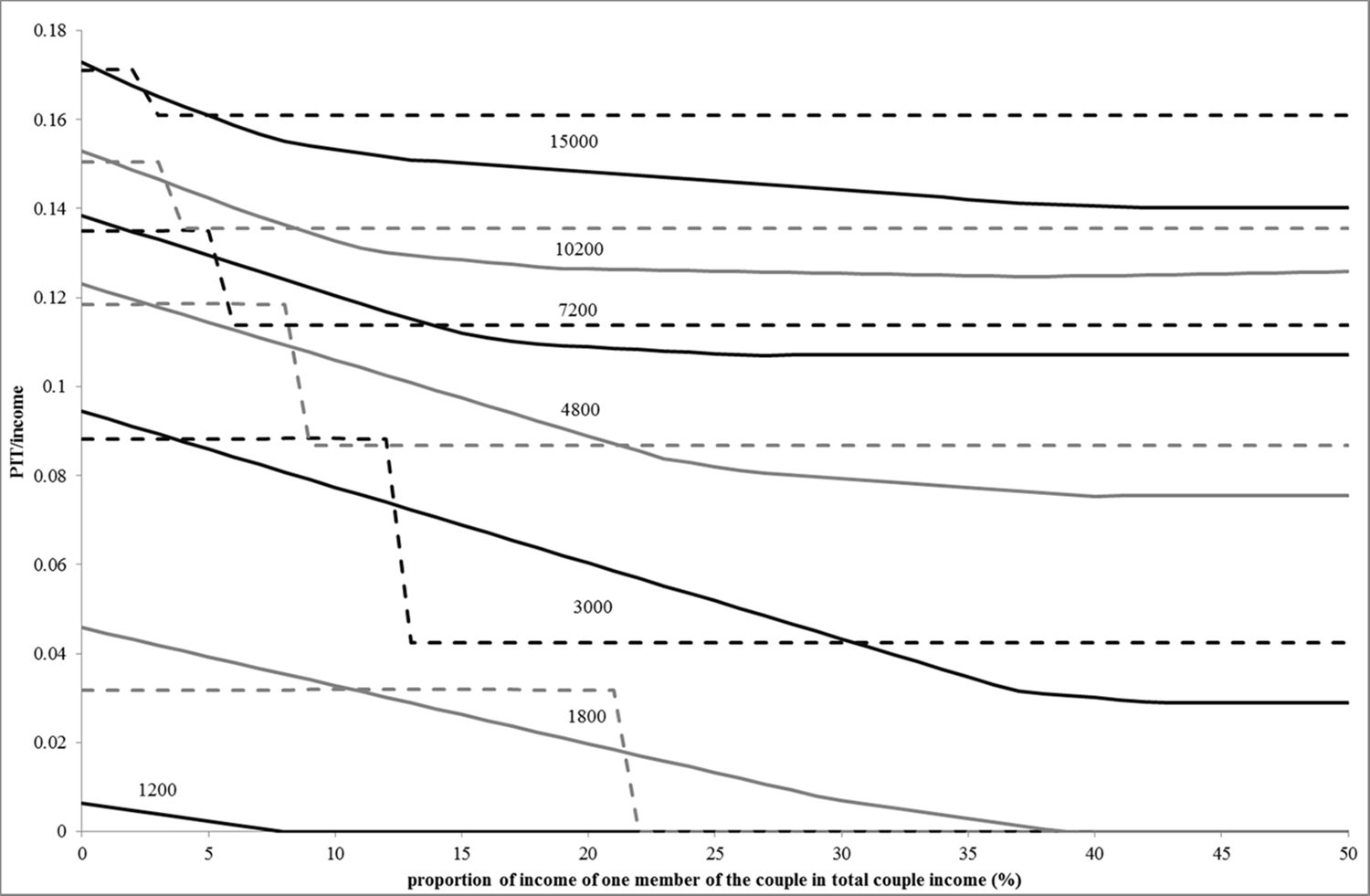
Personal Income Tax-to-income ratio for selected couples by participation of one spouse in generating labour income.
The solid lines depict the path of the tax burden under individual filing as the participation of one spouse in labour market income generation rises. Participation ranges from 0 to 50 per cent, so unsurprisingly the curves are decreasing (or at least non-increasing), reflecting the advantages of sharing labour market activities between spouses.
Source: author’s calculations based on schedule rates.
Note: The tax burden is calculated for different levels of couples’ labour income: US$ 1,200 (close to percentile 12 of the labor income distribution of couples), 1,800 (22), 3,000 (43), 4,800 (66), 7,200 (83), 10,200 (92), 15,000 (97). Dotted lines represent the tax burden under joint filing; solid lines represent the tax burden under individual filing.
The dotted lines show the pattern of the tax burden with one spouse generating labour income under joint filing. We observe that all the joint filing curves show a one-step fall. This is easily explained. The tax schedule under joint filing distinguishes two cases: one is applied when the earnings of at least one spouse are below a threshold (12 times annual minimum wage) and the other one when earnings of both spouses exceed the threshold.
For all levels of labour income of the couples, when only one spouse participates in the labour market, the tax burden of the couple is lower under joint than individual filing. As seen in Figure 2, this holds for the lowest values of the x-axis.
Although the figure does not reflect all possible situations, a first look suggests that the code does not encourage uneven labour market participation between spouses to reach a level of income. Indeed, the most interesting aspect of the curves is that if the couple chooses the least burdensome option (given income), the resulting curve is non-increasing, reflecting that there are advantages to sharing labour market time between spouses, or at least that there are not disadvantages.
Figure 2 also helps to illustrate a gender related issue discussed by Nelson (1991): dedication of women to household services may be encouraged because of the non-recognition of home production as a taxable income. When only one spouse participates in the labour market, household services are provided by the other spouse without facing a burden tax. Meanwhile, the two-earner couple can reach higher levels of labour income and therefore bear a higher burden tax, though it would need for money to pay for market goods to replace home production. For all the income levels reported in Figure 2, we find that the tax burden faced by a one earner couple under joint taxation is lower than the burden faced a by two-earner couple that generates twice as much as the former.
3. Data and methods
3.1. Data and imputations
We use the Household Survey (ECH because of the Spanish abbreviation of Encuesta Continua de Hogares) carried out in 2013 by the National Statistical Office (INE, following the Spanish abbreviation Instituto Nacional de Estadística). It is a nation-wide representative survey that reported information of 46,622 households (89.3 per cent response rate). Among several characteristics of household members, it registers post-tax in-kind and monetary income received in the month before the interview, by source.
Burdin et al., 2014 assess the accuracy of the ECH comparing its information with Tax Office records for the period 2009–2011. To estimate gross income based on ECH, they follow a procedure quite similar to the one used in this paper and described below. They conclude that the ECH underestimates capital income but it is fairly accurate to measure labour income and pensions, though top incomes are not well registered. The ratio between capital income reported by ECH and administrative records had a decreasing trend in the period of study; it was on average 73% but only 48% in 2011. The difference was very important among high income individual for which capital income is noticeable underestimated in data survey. Meanwhile, the average ratio for 2009–2011 was 88% for pensions and 104% for labour income. It is worth to note that in the case of labour income data of the ECH, they only considered the information given by workers who declared to pay contributions of the Social Security System. In other words, they assumed that contributors pay PIT and workers that pay PIT are contributors.
Our variable of interest is the household tax rate measured as household PIT-to-(gross) income ratio. As the ECH asks about income after taxes and contributions, we estimated the individual taxes and contributions using the statutory rates in force in 2013, and we added them to the reported individual income in order to have a proxy of gross income. Then, we calculated the income and the paid PIT of the household adding information of its members, and finally, the household tax rate. We assigned to individuals their household tax rate.
In the case of capital income, we computed the taxable capital gains as the sum of all reported capital income and we assumed that there is no evasion. The ECH does not provide information to estimate tax deductions so we implicitly assumed that conditions for them were not present. This assumption should be tested in the future; anyway, the most important concern related to capital income is the underreporting.
The ECH reports whether or not the worker contributes to the Social Security System. We assumed that there is no partial evasion by contributors and that non-contributors do not pay taxes either[2] as in Burdin et al., 2014. Because of the findings by Vigorito & Esponda when comparing ECH and Tax Office records, we expect that this is a reasonable assumption to estimate gross labour income of workers who do not evade their PIT payments. However we cannot assess the accuracy of labour income reported in the survey by evaders. Regarding PIT credits, we considered contributions and child benefits, but we did not impute deductions related to mortgages and rents due to the lack of information for an appropriate assumption. Credits for children were assigned to the head of the household who is usually the household member who receives the highest income.
When estimating the amount of PIT paid we assumed that individuals opt for individual filing because joint filing is rarely used. Besides, the survey does not provide any information that would help distinguish couples that used different options. Thus, we performed a first analysis using estimations of gross income and PIT based on individual filing. Then, to analyse the effect of the joint filing option we estimated the amount of PIT under joint filing given the already estimated gross income.
To analyse sources of income we deflated them by the Consumer Price Index and classified them into four groups: capital income, labour income, other income (public and private transfers plus self-consumption), and imputed rental value of owner-occupied houses).
3.2. Gendered classification of the population
Personal income taxes are generally applied to individuals. However, studies on inequality and distributive effects of taxes chose the household as the proper unit of analysis under the understanding that household members share income and other resources. As our focus is the analysis of gendered distributive effects, the challenge is to provide an appropriate gender classification of households. To address the issue about the effects on allocation of time between labour market and home production and to take into account lack or time of lone parents, we are interested on identifying the typical cases of one-earner couple, two-earner couple and single female earner. Besides, we want to compare similar types of one-earner couple and single earner but supported by earners of different gender. Finally, in developing countries we have to take into account the existence of extended households (households where there are members related by other links than children or partner such as grand-parents, brothers-in-law, nephews, non-relatives, etc.) whose gendered nature is difficult to be captured.
Thus, we made a classification of the population that takes into account the household structure and the employment status of household members. The classification appears in the first column of Table 2.
Main characteristics of household categories
| Household category | Frequency (weighted cases) (%) | Households with children (%) | Number of members | Number of earners | Lack of contribution to social security (%) | Age of the household head and spouse | Number of cases in the sample |
|---|---|---|---|---|---|---|---|
| All | 100 | 59.8 | 3.7 | 1.9 | 22.5 | 48.9 | 124,987 |
| Couple, male breadwinner | 18.4 | 72.4 | 4.1 | 1.4 | 27.3 | 42.5 | 22,230 |
| Couple, dual earner | 30.7 | 72.1 | 3.8 | 2.3 | 19.9 | 41.4 | 37,082 |
| Couple, female breadwinner | 3.2 | 42.1 | 3.3 | 1.9 | 27.7 | 52.4 | 4,033 |
| Couple, non-employed | 7.0 | 9.1 | 2.6 | 1.7 | 4.5 | 68.5 | 9,008 |
| Single, male breadwinner | 3.2 | 20.1 | 1.7 | 1.2 | 31.6 | 47.1 | 4,125 |
| Single, female breadwinner | 7.8 | 60.6 | 2.9 | 1.5 | 30.4 | 45.2 | 11,225 |
| Single, non-employed male | 1.3 | 3.6 | 1.4 | 1.1 | 3.9 | 70.2 | 1,886 |
| Single, non-employed female | 6.1 | 22.0 | 2.2 | 1.1 | 9.4 | 65.9 | 8,670 |
| Couple, male breadwinner, extended | 4.0 | 83.1 | 5.8 | 2.3 | 34.2 | 48.5 | 4,721 |
| Couple, dual earner, extended | 4.5 | 80.5 | 5.4 | 3.2 | 28.1 | 45.8 | 5,268 |
| Couple, female breadwinner, extended | 0.8 | 70.1 | 5.2 | 2.8 | 31.2 | 56.5 | 943 |
| Couple, non-employed , extended | 2.2 | 65.2 | 5.0 | 2.7 | 14.1 | 66.5 | 2,615 |
| Single, male breadwinner, extended | 1.7 | 37.7 | 3.5 | 2.2 | 30.8 | 44.4 | 1,976 |
| Single, female breadwinner, extended | 4.1 | 71.8 | 4.4 | 2.2 | 33.7 | 47.9 | 5,113 |
| Single, non-employed male, extended | 0.8 | 50.1 | 3.9 | 2.0 | 19.2 | 65.6 | 974 |
| Single, non-employed female, extended | 4.2 | 62.8 | 4.3 | 2.2 | 20.1 | 65.8 | 5,118 |
-
Source: Authors’ calculations based on Encuesta Continua de Hogares 2013, Instituto Nacional de Estadística.
-
Note: The lack of contribution to social security is calculated at household level as the ratio between non-contributors and workers; the ratio takes value 0 when no one in the household participates in the labour market.
We first distinguish extended from non-extended households (that are comprised of single individuals or couples, with or without children at any age). We distinguish eight household types within each group. In the rest of the paper we focus on the eight types of non-extended households.
Three categories represent the typical cases that are of interest from the gender perspective of tax studies. The “couple, male breadwinner” category includes non-extended households formed by a couple (with or without children) in which only the male participates in the labour market. Around 19 per cent of individuals live in this type of household. The “single, female breadwinner” category consists of a non-extended household headed by a single worker woman, and accounts for 7.8 per cent of population. The “couple, dual earner” category corresponds to non-extended households formed by a couple in which both the male and female work in the labour market. This category is the most frequent, accounting for 30.7 per cent of individuals.
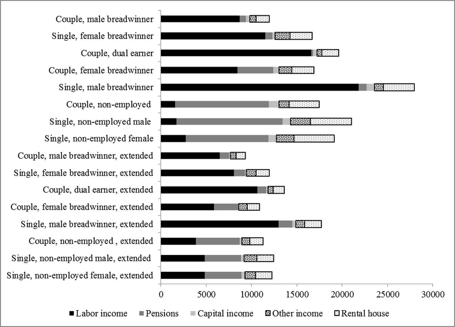
As reported in Table 2, most of the households in these three categories have children and the average age of the adults is fairly similar. In turn, as shown in Figure 3, the “couple, dual earner” category has the highest per capita income of the three types. Labour income is the most important source in all three categories and public transfers are more important for the “single, female breadwinner” type than for the others.

Per capita income of households by source.
Source: Authors’ calculations based on Encuesta Continua de Hogares 2013, Instituto Nacional de Estadística.
3.3. Empirical strategy
We aim to identify gender differences in the PIT burden and also to examine the role of some specific household characteristics in the explanation of those differences. A particular issue in our study is that the main variable of interest, the PIT-to-income ratio, includes many observations of 0 and no 1 seconds (no household is taxed at 100%). These zeros can provide important information for the study of the lowest levels of taxation and they are included for theoretical and empirical reasons. Hence, we conduct the empirical analysis considering a dependent variable that assumes values in the interval [0, 1) and contains excess of zeros.
In a case like this, the dependent variable is not symmetrically distributed, so the predicted values of the linear regression model may lie outside the unit interval. As an alternative, Cook et al. (2008) proposed the zero-one inflated beta model (ZOIB) which properly addresses the issue related to the inflation process in the data.
Several authors (Paolino, 2001; Kieschnick and McCullough, 2003; Smithson and Verkuilen, 2006) argue that the beta regression model is the most suitable for distributional asymmetries and can be adjusted for data in the interval (0, 1) since the density function takes different shapes depending on the function parameters. Ferrari and Cribari-Neto (2004) proposed the following parameterization for the density function of the response variable y when it adopts a beta distribution Β(μ, ϕ):
where µ is the mean (0 < µ<1), ϕ a precision parameter (ϕ>0) and Γ(.) is the gamma function.
In practice, the beta distribution is not suitable for modelling data that contains zeros or ones. But we want to consider observations where the dependent variable is zero. Therefore, we apply a combination of two distributions: a beta distribution when the variable is bounded by 0 and 1, and another distribution function that is in effect when the variable takes the value 0. For a detailed description of this methodology see Ospina and Ferrari (2010), Ospina and Ferrari, 2012). The density is called a zero-inflated beta distribution and the probability function generated by the combination is:
In this paper, we carry out all the estimations using the Stata module zoib developed by Buis (2012).[3] The zoib command consists of a maximum likelihood estimation of the combined model: a logistic regression of whether or not the income share paid to taxes equals zero and a beta regression for the proportions in the interval (0, 1). We perform all the estimations using robust standard errors.
Our explanatory variable of interest is a vector of dummy variables that captures household type, which provides the gendered classification of the population. We also use several variables that reflect household characteristics: the household per capita income, a dummy variable that takes a value equal to one when there is at least one member younger than 18 in the household, the household size, the number of earners per household and the lack of contribution to social security measured as the ratio of the number of workers that are not contributors and the number of workers in the household (the ratio takes value 0 when there are no workers in the household). Additionally, we break down the household income by source in order to separately capture the incidence of all sources: capital income, labour income, pensions, other income (public and private transfers plus self-consumption) and rental value. The choice of these variables responds to the fact that they may explain differences in the PIT burden due to the characteristics of the tax detailed in Section 2.2. In particular, we aim to capture progressivity, the treatment to the different sources of income and the design of credits and deductions.
We compute and report the marginal effects of the dependent variables on the PIT-to-income ratio. In the case of the household type vector, the effect is the discrete effect of moving from “couple, dual earner” to each respective other household type. For the other variables, the effect is measured for the “couple, dual earner” household, valuing the rest of the variables at their mean.
4. Results
4.1. Tax incidence analysis
The PIT is a progressive tax. Its Kakwani index is positive (0.360) and the Gini index declines from 0.426 pre-tax to 0.413 post-tax, reflecting the PIT’s equalizing effect. However, the distributive effect is limited because of the tax size and exemptions. Around 54% of the population lives in households that do not pay the tax, and the average PIT burden is 1.8% population wide and 3.9% among the population of households who face this tax.
In Figure 4 we present the PIT incidence by household type. The dark bar shows the average burden and the pale bar shows the proportion of non-taxpayers; for both variables, a straight line indicates the 95% confidence interval of the estimation.

Average PIT burden and proportion of non-taxpayers by household type
Source: Authors’ calculations based on Encuesta Continua de Hogares 2013, Instituto Nacional de Estadística.
Note: in each bar, the straight line indicates the 95% confidence interval of the estimation.
At the top we show the five types of non-extended working households. The “couple, dual earner” category bears the largest PIT burden (2.4%) and has the highest proportion of taxpayers (61%). The “couple, dual earner” category is followed by male breadwinner households which have an average burden of 2% when living with no partner and 1.8% when living with a partner. Finally, the lowest burden corresponds to female breadwinner types: 1.5% when in union or married and 1.2% when single.
The PIT burden is lower for non-employed households than households of workers. Among the latter ones, the highest tax incidence corresponds to the “couple, non-employed” type with an average burden of 1.5% whereas the single types pay an average of 1% of income in the form of the PIT. There are no significant gender differences between single types.
We report the PIT incidence for extended households following the same order as for non-extended households. The tax burden is lower among extended households. The gender differences within extended households are similar to those already depicted.
4.2. Exploring differences among non-extended workers’ households
We analyse the tax burden differences between household types through the estimation of a ZOIB model. We include sixteen dummy variables that distinguish household types, but in this section we only show the results for the household types of interest.
In Table 3 we report the discrete effect of the household type relative to the “couple, dual earner” type. In column Model one we show the results of an estimation in which we do not include any control. Thus, these estimated effects replicate the patterns of the raw PIT burden differences already shown: all effects are negative, indicating that the dual earner type has a higher PIT-to-income ratio, and that male types have a higher ratio than female types regardless of whether comparing singles or couples.
Marginal effects estimated by a zero-inflated beta regression
| Variables | Model 1 | Model 2 | Model 3 |
|---|---|---|---|
| Couple, male breadwinner | −0.0067*** (0.00005) |
0.0048*** (0.00007) |
0.0046*** (0.00007) |
| Single, female breadwinner | −0.0116*** (0.00006) |
−0.0141*** (0.00006) |
−0.0056*** (0.00007) |
| Couple, female breadwinner | −0.0084*** (0.00008) |
−0.0071*** (0.00008) |
0.0035*** (0.00009) |
| Single, male breadwinner | −0.0045*** (0.00010) |
−0.0184*** (0.00006) |
−0.0150*** (0.00010) |
| Per capita income | 0.0205*** (0.00004) |
||
| Presence of children (yes =1) | 0.0082*** (0.00004) |
||
| Household size | 0.0041*** (0.00002) |
||
| Number of earners (labour, capital earnings or pensions) | −0.0044*** (0.00003) |
||
| Lack of contribution to social security | −0.0001*** (0.00000) |
||
| Per capita capital income | 0.0574*** (0.00075) |
||
| Per capita labour income | 0.0286*** (0.00008) |
||
| Per capita pension | 0.0278*** (0.00009) |
||
| Per capita public transfer | −0.0036*** (0.00012) |
||
| Per capita imputed rent of owner-occupied house | −0.0051*** (0.00011) |
||
| Observations | 124,987 | 124,987 | 124,987 |
-
Source: Authors’ estimations based on Encuesta Continua de Hogares 2013, Instituto Nacional de Estadística.
-
Note: For household types, we report the discrete effect related to the “couple, dual earner” type, valuing the rest of the variables at their means. For the rest of the dependent variables, we report the ‘marginal effect’ by household type compared to the “couple, dual earner” type.
-
***p<0.01, **p<0.05, *p<0.1
The purpose of the PIT is progressivity, so a proper analysis needs to control the results by income. Thus, we estimate Model two in which we add per capita gross income as a control. As expected, the PIT burden increases with income. The difference in income levels by household type affects the order of the three typical cases: now, the “couple, male breadwinner” type has the highest PIT-to-income ratio, followed by “couple, dual earner” and “single, female breadwinner”.
These results are consistent with gender equality although we do not know (and we do not address the study of) the optimal magnitude of the gaps. The lower tax burden among dual earner than among male breadwinner households does not discourage female labour market participation. Also, there would be a fairness concern if the one earner household receives a better treatment than a female without a spouse. Nelson’s argument is behind this gender equity concept: given income, welfare depends on the capacity of household’s production which is not taxed.
Besides the three typical types, there are two other comparisons that may help to understand gender differences: “couple, male breadwinner” vs “couple, female breadwinner” and “single, female breadwinner” vs “single, male breadwinner”. Both female types bear a lower tax burden than male types.
To analyse the PIT ratio differences between household types, we estimate Model three in which we include possible sources of those differences: presence of children, household size, number of earners and the lack of contribution to social security (a proxy of the percentage of worker tax evaders in the household). Also, the explanatory variable of income is split into several sources. As shown in Table 3, even after including all the variables that may explain the differences, the gaps decline although they do not vanish. .
Let’s analyse the demographic controls. The tax burden is higher when there are children in the household and increases with household size. This result is not surprising: on the one hand, the tax burden is likely to increase with total household income because of the progressivity of marginal tax rates on pensions and labour earnings; on the other hand, in each level of per capita household income, total income of the household increases with its size. As the average values of household size and presence of children are higher for “couple, male breadwinner” than “couple, dual earner”, the PIT burden tends to be higher for the former
We interpret that the presence of children and the household size are demographic characteristics mainly related to life-cycle stage. But tax evasion and the income sources are at least partially influenced by culture and socioeconomic arrangements, so the interpretation of the PIT ratio differences should be interpreted cautiously from a gender perspective.
The effect of the number of earners is negative because of the progressivity of marginal taxes. I.e., at a given level of income, the PIT-to-income ratio is lower when the number of members receiving income is higher. As the number of earners is lower in the “couple, male breadwinner” category than the “couple, dual earner” category, the variable contributes to a higher gap between these types.
Unsurprisingly, the lack of contribution (tax evasion) has a negative effect. As it is higher in “couple, male breadwinner” than in “couple, dual earner” households, different behaviour patterns in tax evasion do not contribute to explain the tax burden gap.
Finally, the marginal effects by income source indicate that the tax burden decreases when households are supported by non-taxable income (transfers and rental value). These sources are very important within the female type households so they contribute to explain their lower PIT burden. Public transfers are an important part of the non-taxable income. In Uruguay, most of the public programs of monetary transfers are directed to low-resources families. So, our findings suggest that the incidence of low income households is higher among female than male types. The share of non-taxable income is 13% among “couple, dual earner” but 25% for “single, female breadwinner”. In turn, for the “single, male breadwinner”, which tax burden is higher than its female counterpart, the non-taxable income accounts for 16% of their income. Finally, the incidence of non-taxed income for “couple, female breadwinner” (22%) is higher than for “couple, male breadwinner” (18%).
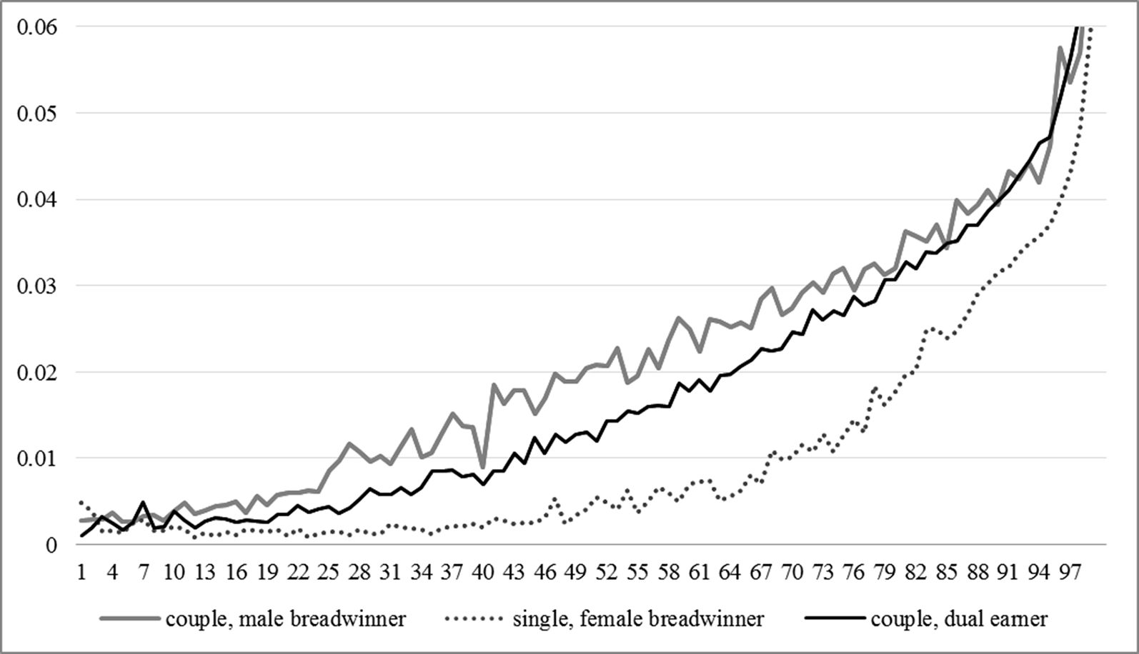
These results reflect the average situation. We also did an estimation based on Model three in which the household type is interacted with all the income sources. In Figure 5 we report the predicted PIT burden across the per capita income distribution for “couple, dual earner”, “couple, male breadwinner” and “single, female breadwinner”. The average depicted pattern is clearly identified in the central range of the income distribution: between the 25th and 75th percentile, the “couple, male breadwinner” type bears the highest burden whereas the “single, female breadwinner” exhibits the lowest one. But over the 75th percentile, the difference between the curves for the “couple, dual earner” and the “couple, male breadwinner” categories are not statistically significant at conventional levels. Meanwhile, “single, female breadwinner” has the lowest burden level across the entire distribution, although the magnitude of the gap is lower at the tails.

Predicted PIT across percentiles of per capita income distribution for three selected household types.
Source: Authors’ estimations based on Encuesta Continua de Hogares 2013, Instituto Nacional de Estadística.
4.3. Introducing joint taxation
Up to now we assumed that all individuals opt for individual filing. In this section we estimate the PIT amounts that would be paid under joint filing if we assume that couples choose the lowest burden option. Remind that we estimated that 5.4% of couples in the Tax Office records chose joint filing in 2013. In our simulation we find that 17% of the households with a labour income source (12% of total households) would benefit by choosing joint instead of individual filing. Thus, this estimation is much higher than the one based on tax records.
According to our simulation, joint filing is not only the best choice for the “couple, male breadwinner” type but also for one quarter of the “couple, dual earner” households in the database that pay PIT.
To analyse the potential effect of the joint filing option we estimate each model assuming that couples choose their best option. The results are reported in Table 4.
Marginal effects estimated by a zero-inflated beta regression
| Variables | Model 1 | Model 2 | Model 3 |
|---|---|---|---|
| Couple, male breadwinner | −0.0086*** (0.00004) |
0.0022*** (0.00006) |
0.0025*** (0.00007) |
| Single, female breadwinner | −0.0107*** (0.00006) |
−0.0123*** (0.00006) |
−0.0031*** (0.00007) |
| Couple, female breadwinner | −0.0095*** (0.00008) |
−0.0081*** (0.00007) |
0.0016*** (0.00010) |
| Single, male breadwinner | −0.0036*** (0.00010) |
−0.0164*** (0.00006) |
−0.0122*** (0.00010) |
| Per capita income | 0.0201*** (0.00004) |
||
| Presence of children (yes =1) | 0.0084*** (0.00004) |
||
| Household size | 0.0045*** (0.00002) |
||
| Number of earners (labour, capital earnings or pensions) | −0.0044*** (0.00003) |
||
| Lack of contribution to social security | −0.0001*** (0.00000) |
||
| Per capita capital income | 0.0665*** (0.00089) |
||
| Per capita labour income | 0.0299*** (0.00007) |
||
| Per capita pension | 0.0302*** (0.00009) |
||
| Per capita public transfer | −0.0032*** (0.00013) |
||
| Per capita imputed rent of owner-occupied house | −0.0054*** (0.00011) |
||
| Observations | 124,987 | 124,987 | 124,987 |
-
Source: Authors’ estimations based on Encuesta Continua de Hogares 2013, Instituto Nacional de Estadística.
-
Note: For household types, we report the discrete effect related to the “couple, dual earner” type, valuing the rest of the variables at their means. For the rest of the dependent variables, we report the ‘marginal effect’ by household type compared to the “couple, dual earner” type.
-
***p<0.01, **p<0.05, *p<0.1
The patterns between models are similar to those obtained under the assumption of individual filing. Model two indicates that the “couple, male breadwinner” type bears the highest burden, followed by “couple, dual earner” and “single, female breadwinner”. But the gap between “couple, male breadwinner” and “couple, dual earner” is smaller than under individual filing. This suggests that joint filing helps to offset the incentives of sharing labour market work between spouses implicit in individual filing. Also the difference between “single, female breadwinner” and “couple, dual earner” becomes smaller. This is due to the gains for some “couple, dual earner” households opting for joint filing.
4.4. The tax burden of non-employed
The estimation of Model two indicates that the “couple, non-employed” type bears a lower burden than the “couple, dual earner” type (a significant marginal effect of –0.0087). This difference between types responds mainly to the fact that households of non-employed are formed by small households of elders. Thus, a similar per capita income means a higher total income for the “couple, dual earner” type. Once we control by the demographic variables, the marginal effect of “couple, non-employed” is positive. Indeed, the elders tend to face a higher PIT burden because they are more likely supported by pensions and capital income than labour income.
In Table 5 we present the estimated effect of the “single, non-employed” types relative to the “couple, non-employed” type. The negative effects indicate that among non-employed households, the couple type has the highest burden. The interest for our purpose is that the difference between the female and male types is small in all models – ie, the PIT seems to not have different gendered treatment among the non-employed.
Marginal effects estimated by a zero-inflated beta regression
| Variables | Model 1 | Model 2 | Model 3 |
|---|---|---|---|
| Single, non-employed female | −0.0045*** (0.00013) |
−0.0103*** (0.00007) |
−0.0128*** (0.00016) |
| Single, non-employed male | −0.0049*** (0.00007) |
−0.0105*** (0.00006) |
−0.0122*** (0.00011) |
| Controls | No | Yes | Yes |
| Observations | 124,987 | 124,987 | 124,987 |
-
Source: Authors’ estimations based on Encuesta Continua de Hogares 2013, Instituto Nacional de Estadística.
-
Note: The vector of household types includes 16 categories (presented in Table 2); for the estimation we omitted “couple, non-employed”. The rest of the variables are valued at mean. Models 2 and 3 include the control variables shown in tables 3 and 4.
-
***p<0.01, **p<0.05, *p<0.1
In Figure 6 we present the predicted PIT burden across the per capita income distribution, calculated based on Model 3. The average pattern holds for all ranges of the per capita income distribution: we do not find gender differences.

Predicted PIT across percentiles of per capita income distribution for three selected household types
Source: Authors’ estimations based on Encuesta Continua de Hogares 2013, Instituto Nacional de Estadística.
5. Conclusions
Gender issues have been debated in the policy agenda of social security system and led to some modifications such as the use of similar mortality rates for women and men to calculate the retirement pension, and the computation for women of one year per child in the calculus of the number of years of contribution required to retire. Feminist movements also claim the reduction of indirect taxes is some female goods, especially the ones linked to reproductive health.
In this study, we analyse the gendered effects of the PIT in Uruguay. The PIT was introduced ten years ago by a left government and the discussions about it (before and after its creation) are centred on its distributive effect. However, gender equity has not been raised in this debate.
The analysis of the legislation indicates that there are no explicit gender differences in the code, which means that the PIT treats women and men on an equal basis regarding rates, credits and deductions. There is a flat tax rate for capital income and two different progressive schedules for pensions and labour income. It is a joint filing system though joint system is allowed for couple income. On the base of Tax records we estimate that only 5.4% of couples (with at least one labour income earner) used the joint filing option in 2013. This low incidence may be explained by the lack of incentives to opt for joint filing. However, on the base of survey data, we estimate that 17% of couples (with at least one labour income earner) would benefit for joint filing. We cannot assess the difference between these two estimations. Note that there are not simple rules (such ranges of income level or ranges of participation of one spouse in the couple’s labour income), except the case of one earner couples, to inform the population who benefit or not of joint filing. Thus, a possible explanation of the discrepancy is lack of information. Indeed, every year couples have to calculate their PIT payments under individual and joint filing to opt for the least costly. But there are probably other explanations that could be the scope of future research.
We conduct the analysis using microdata provided by the 2013 Household Survey. We estimated taxes and contributions using the statutory rates in force in 2013. There is an important limitation of the survey because of the underreporting of capital income ( Burdin et al., 2014) whereas there are no assessments about the accuracy of the labour income reports of evader workers. Besides, as it informs income after taxes, we made several assumptions to estimate gross income. The most important are the ones related to evasion: we assume no evasion of income capital and full evasion of labour income when there is not contribution to the social security system. The evasion assumption related to labour income seems no to be too unrealistic: Burdin et al., 2014 find that the aggregated labour income obtained under this assumption is similar to the total labour income informed by Tax Office records. However, the assumption of no evasion of income capital may be extreme and could bias the results: the highest share of income capital is observed for non-employed households (both single male and female) and one earner households (male and female breadwinner types). Future analysis should work on the underreporting and evasion of capital income and assess the sensitivity of the results to these issues.
The raw data indicate that households in which both spouses participate in the labour market bear the highest PIT burden followed by the typical patriarchal household in which the husband works in the labour market but not the wife. But his order changes when we control by household per capita income. Households supported by a working man who lives with a dependent housewife face the highest tax burden, followed by the dual-earner type. This finding is similar to the obtained for Argentina ( , 2018) and eight countries (Argentina, United Kingdom, Ghana, Uganda, Morocco, South Africa, Mexico and India) (Grown and Valodia, 2010). When we control by different potential explanatory factors, a gap remains. One of the factors that explain the gap is the lower number of earners of male breadwinner households which is consequence of the individual filing design. But even in the analysis of the joint filing design, the PIT burden is higher for male breadwinner than dual earner households.
These findings indicate that there is an incentive towards equal gender time allocation within the family, which is consistent with gender equity. On one hand, PIT does not discourage labour market participation of a second earner due that it is not taxed at higher rates. On the other hand, given that male breadwinner households may reach higher levels of welfare from non-taxed home production, the result is potentially not inconsistent with neutrality in terms of allocation between household and market time. However we cannot assess the magnitudes of the estimated PIT burden gaps. We made an exercise in which we compare the tax burden of a one earner couple under joint taxation and a two-earner couple under individual couple. We assumed that the three earners of the example generated the same level of labour income and the fourth individual, a similar value of home production. For different income level, we obtained that the one earner couple has a lower PIT burden than the two earner couple. Thus, the assessment of gap magnitudes appears to be a relevant topic for further research.
Single mother households bear a lower burden than dual earner households when considering both raw data and income controlled gaps. Once again, this pattern is consistent with gender equity.
However, this pattern is partly explained by non-desirable aspects: the higher levels of informality and participation of non-taxable sources of income among single female households than dual earner households.
We also compare male and female breadwinner households, and single female and male households. In both comparisons we find that the male types bear a higher PIT burden than the female types, which is partly explained by the higher share of non-taxable income among female types. We also study three typical types of non-employed households and we do not find differences between female and male categories.
Our findings may contribute to the debate of future reforms of the PIT. In fact, once in a while there are social pressures to reduce taxes to alleviate the burden on families. The question is if a new design could worsen horizontal equality from a gender perspective. For example, it is not advisable to allow exemptions for dependant spouses but it would be helpful to take into account persons unable to support themselves. Also to eliminate the option for actual joint filing would improve equality and, on the other sides, changes in the schedule rate of the actual joint filing should be carefully assessed.
Footnotes
1.
Percentile values were provided by the Economic Institute of the Faculty of Management, Universidad de la República and are based on administrative records of the Tax Office.
2.
The ECH inquires whether or not private wage earners partially evade social security contributions. We did not take into account this information because it would require further assumptions about the percentage of evasion. In any case, we do not expect that assumptions about partial evasion based on this information have significant effects on our results: 58% of workers were private wage earners and among them, only 6% declared to partially evade.
3.
We also run OLS estimations that are available by request. The estimated effects have the same signs than under the zoib estimation though the magnitudes are a bit different.
References
-
1
Gender-Based taxation and the division of family choresAmerican Economic Journal: Economic Policy 3:1–40.https://doi.org/10.1257/pol.3.2.1
-
2
La segregación ocupacional de género y las diferencias en las remuneraciones de los asalariados privados. Uruguay, 1990-2000Desarrollo Económico 44:109–129.https://doi.org/10.2307/3455869
-
3
Gender bias in Tax systems based on household incomeAnnals of economics and statistics 117/118:141–155.https://doi.org/10.15609/annaeconstat2009.117-118.141
- 4
-
5
Family labor supply, taxation and saving in an imperfect capital marketReview of Economics of the Household 8:297–323.https://doi.org/10.1007/s11150-010-9094-1
-
6
Taxation of married couples in Germany and the UK: One-earner couples make the differenceInternational Journal of Microsimulation 6:3–24.
-
7
Strengthening a fiscal Pillar: the Uruguayan dual income taxCEPAL Review 2007:121–140.https://doi.org/10.18356/126c5701-en
-
8
Revealing Gender Gap Changes in Home Production and Labor Income in Uruguay WP 5/18Departamento de Economía, Facultad de Ciencias Sociales, UDELAR.
-
9
Salarios femeninos en Uruguay: ¿existe un techo de cristal?Revista de Economía 12:63–88.
-
10
ZOIB: Stata module to fit a zero-one inflated beta distribution by maximum likelihoodStatistical Software Components.
-
11
Desigualdad Y altos ingresos en Uruguay. un análisis en base a registros tributarios Y encuestas de hogares para El período 2009-2011. Serie Documentos de Trabajo, DT 06/2014, Instituto de Economía, Facultad de Ciencias Económicas y AdministraciónDesigualdad Y altos ingresos en Uruguay. un análisis en base a registros tributarios Y encuestas de hogares para El período 2009-2011. Serie Documentos de Trabajo, DT 06/2014, Instituto de Economía, Facultad de Ciencias Económicas y Administración.
-
12
Sectores de altos ingresos en Uruguay: participación relativa y patrones de movilidad en el período 2009-2012, Serie Documentos de Trabajo, DT 03/2015, Instituto de Economía, Facultad de Ciencias Económicas y AdministraciónUruguay: Universidad de la República.
-
13
Regression analysis of proportions in finance with self selectionJournal of Empirical Finance 15:860–867.https://doi.org/10.1016/j.jempfin.2008.02.001
-
14
Budgeting for women´s rights: monitoring government budgets for compliance with CEDAWNew York: UNIFEM.
-
15
Brechas salariales en Uruguay: género, segregación y desajustes por calificaciónRevista Problemas del Desarrollo 174:89–117.
-
16
Desigualdades persistentes: mercado de trabajo, calificación y género. El futuro en foco: Cuadernos sobre Desarrollo HumanoMontevideo: PNUD.
-
17
Beta regression for modelling rates and proportionsJournal of Applied Statistics 31:799–815.https://doi.org/10.1080/0266476042000214501
-
18
Moving towards dual income taxation in EuropeFinanzArchiv 63:436–456.https://doi.org/10.1628/001522107X250140
-
19
Taxation and Gender Equity: A comparative analysis of direct and indirect taxes in developing and developed countriesTaxation and gender equality. A conceptual framework, Taxation and Gender Equity: A comparative analysis of direct and indirect taxes in developing and developed countries, London, Routledge, Chapter 1.
-
20
Gender Equity and Taxation in Latin America and the Caribbean, Comparative Chapter. Non-publishedGender Equity and Taxation in Latin America and the Caribbean, Comparative Chapter. Non-published.
-
21
Taxation and Gender Equity: A comparative analysis of direct and indirect taxes in developing and developed countriesLondon: Routledge.
-
22
Taxation and household labour supplyThe Review of Economic Studies 79:1113–1149.https://doi.org/10.1093/restud/rdr049
-
23
Regression analysis of variates observed on (0, 1): percentages, proportions and fractionsStatistical Modelling: An International Journal 3:193–213.https://doi.org/10.1191/1471082X03st053oa
-
24
Tax reform and feminist theory in the United States: incorporating human connectionJournal of Economic Studies, 18, 10.1108/EUM0000000000158.
-
25
Inflated beta distributionsStatistical Papers 51:111–126.https://doi.org/10.1007/s00362-008-0125-4
-
26
A general class of zero-or-one inflated beta regression modelsComputational Statistics & Data Analysis 56:1609–1623.https://doi.org/10.1016/j.csda.2011.10.005
-
27
Maximum likelihood estimation of models with beta-distributed dependent variablesPolitical Analysis 9:325–346.https://doi.org/10.1093/oxfordjournals.pan.a004873
-
28
Taxation and Gender Equity: A comparative analysis of direct and indirect taxes in developing and developed countriesGender equality and taxation in Argentina, Taxation and Gender Equity: A comparative analysis of direct and indirect taxes in developing and developed countries, London, Routledge, Chapter 3.
-
29
Equidad de género del sistema tributario en la Argentina: estimación de la carga fiscal desglosada por tipo de hogarRevista de la CEPAL, 124.
-
30
A better lemon squeezer? maximum-likelihood regression with beta-distributed dependent variablesPsychological Methods 11:54–71.https://doi.org/10.1037/1082-989X.11.1.54
- 31
Article and author information
Author details
Funding
No specific funding for this article is reported.
Acknowledgements
Not applicable.
Publication history
- Version of Record published: August 31, 2019 (version 1)
Copyright
© 2019, Bucheli and Olivieri
This article is distributed under the terms of the Creative Commons Attribution License, which permits unrestricted use and redistribution provided that the original author and source are credited.